Quantum simulation of traversable wormhole spacetimes in a Bose-Einstein condensate
Jes\'us Mateos, Carlos Sab\'in

TL;DR
This paper proposes a method to simulate traversable wormhole spacetimes using Bose-Einstein condensates, enabling experimental exploration of exotic spacetime geometries in controlled laboratory settings.
Contribution
It introduces a novel approach for quantum simulation of wormholes in BECs, detailing the required modulation of sound speed and external magnetic fields in different dimensions.
Findings
Feasible modulation of sound speed in 1+1D BECs for wormhole simulation.
Specific magnetic field configurations identified for 3+1D simulations.
Analysis of experimental conditions for implementing the simulation.
Abstract
In this work we propose a recipe for the quantum simulation of traversable wormhole spacetimes in a Bose-Einstein condensate, both in and . While in the former case it is enough to modulate the speed of sound along the condensate, in the latter case we need to choose particular coordinates, namely generalized Gullstrand-Painlev\'e coordinates. For weakly interacting condensates, in both cases we present the spatial dependence of the external magnetic field which is needed for the simulation, and we analyze under which conditions the simulation is possible with the experimental state-of-the-art.
Click any figure to enlarge with its caption.
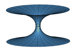 Figure 1
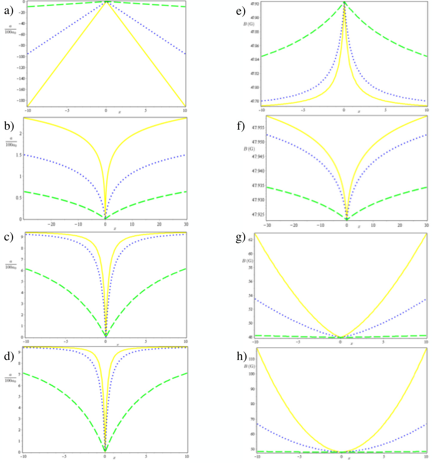 Figure 2
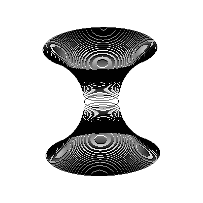 Figure 3
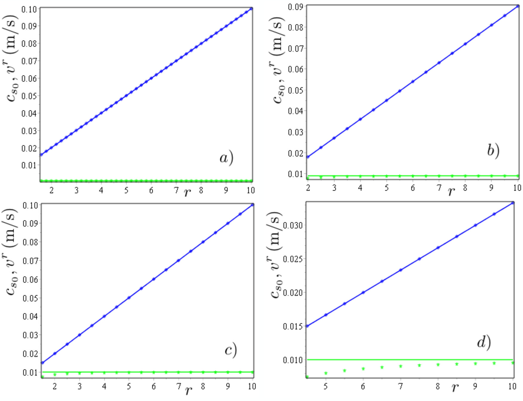 Figure 4
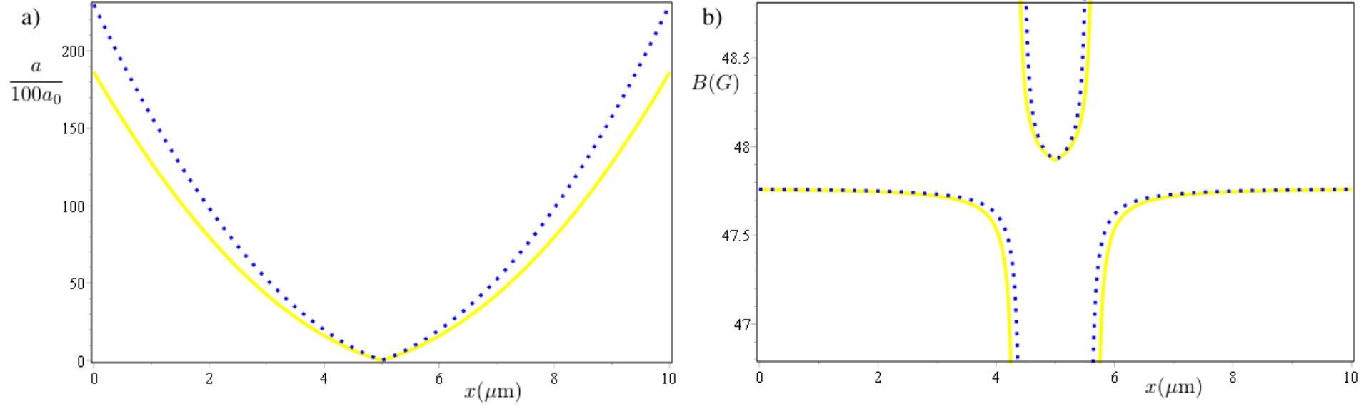 Figure 5
| Atom | ||
|---|---|---|
| Li | ||
| Na | ||
| K | ||
| Rb | ||
| Cs |
Peer Reviews
No public reviews on file for this paper yet. If you reviewed it on a platform where reviews are public (OpenReview, ICLR, NeurIPS, ICML), you can paste yours below so the community can read it here.
Videos
No videos yet. Explain this paper in a talk, walkthrough, or lecture? Add one.
Quantum simulation of traversable wormhole spacetimes in a Bose-Einstein condensate
Jesús Mateos
Facultad CC. Físicas, Universidad Complutense of Madrid,Plaza Ciencias, 1 Ciudad Universitaria 28040 Madrid (Spain)
Carlos Sabín
Instituto de Física Fundamental, CSIC, Serrano, 113-bis, 28006 Madrid (Spain)
Abstract
In this work we propose a recipe for the quantum simulation of traversable wormhole spacetimes in a Bose-Einstein condensate, both in and . While in the former case it is enough to modulate the speed of sound along the condensate, in the latter case we need to choose particular coordinates, namely generalized Gullstrand-Painlevé coordinates. For weakly interacting condensates, in both cases we present the spatial dependence of the external magnetic field which is needed for the simulation, and we analyze under which conditions the simulation is possible with the experimental state-of-the-art.
I Introduction
Quantum simulators enable to study properties of quantum systems which are otherwise out of experimental reach, by mimicking them with more experimentally amenable quantum systems. In this sense, among other possible approaches, they may be thought of as a window to the analysis of physics lying at the edges of the theory zitterbewegung ; Sabin2 ; gws2 , and even beyond majoranas1 ; majoranas2 ; tachions1 ; tachions2 .
Traversable wormholes are interesting cosmological objects which appear in certain solutions of general relativity equations. In principle, they connect distant regions of the universe, or even regions of different universes. Due to this behavior as a spacetime shortcut, they are the focus of great theoretical interest, and they are used as a pedagogical tool in general relativity Thorne ; Thorne2 ; Libro1 ; Libro2 . In particular, they are proposed and studied like a way for interstellar travels Thorne . Recently, they have generated renewed attention as possible “black hole mimickers” gravastar ; konoplya .
However, today their existence has not been demonstrated in a direct or indirect observational way. Moreover, it seems that they do not appear naturally in our universe, and there are theoretical reasons to expect that they must be forbidden Hawking . Indeed, in order for these objects to be stable, they must be made of exotic material which violate the weak energy condition Thorne ; Thorne2 and these spacetimes may contain closed timelike curves (CTCs), which might imply a violation of the principle of causality Thorne2 . In this sense, a quantum simulator can be a useful tool in the analysis of traversable wormholes. Indeed, recently one of us has proposed a quantum simulator of a traversable wormhole spacetime by means of a dc-SQUID array Sabin1 . This proposal was restricted to and to a particular type of wormhole, namely the Ellis wormhole.
Bose-Einstein condensates (BEC) haven been used widely in quantum simulation of cosmological objects, namely black holes Garay1 ; Garay2 or gravitational waves Sabin2 .
In this work, we show how to simulate a variety of traversable wormhole spacetimes in a BEC, both in –where we go beyond the Ellis wormhole case– and in the more realistic case. In the former case, it is enough to modulate the speed of sound along the condensate by means of a Feshbach resonance. In the latter, we introduce particular coordinates to achieve the simulation, namely generalized Gullstrand-Painlevé (GP) coordinates. We will analyze in detail the prospects for an experimental implementation with current technology.
II Traversable wormhole spacetimes
We start from the line element of a traversable wormhole spacetime, which is given by Thorne ; Sabin1
[TABLE]
where is the redshift function and is the shape function, and both functions depend on the radius only. The features of the wormhole are fully determined by these two functions. In particular, and can be adjusted in order to allow a travel trough the wormhole. In the case of the shape function, there exists a value such that , which determines the position of the wormhole’s throat. It defines the proper radial distance to the throat as , which defines two different regions into the same universe for , corresponding to going from to , and , corresponding to going from to . Therefore, when , we have two asymptotically flat regions corresponding to , which are connected through the wormhole throat at , i.e. at . The embedding diagram of Fig. 1 shows a pictorial way to understand these concepts.
For simplicity, we will study a massless wormhole, i.e. , and therefore the expression (1) reduces to
[TABLE]
and now the wormhole is characterized by only.
On the other hand, the effective metric of a BEC in dimensions is a curved metric, which is given as follows Sabin2 ; Fagno ; Visser1
[TABLE]
where is the real spacetime metric in which the condensate is, that it can be curved in general. In our case we take , where is the flat Minkowski metric (note that in this work we choose the “mostly plus” convention for the signature of ). Furthermore, is the density of the BEC, is the phonon propagation speed in the condensate, and is the velocity flow 4-vector, which is associated to the 4-divergence of the BEC’s phase Fagno .
In order to simulate a traversable wormhole in the BEC, the aim is to relate the effective metric (3) with (2).
III case
For simplicity, we work first with the dimensional case. Here, we can leverage the conformal invariance of the Klein-Gordon equation in . The line element (1) becomes
[TABLE]
that is conformal to
[TABLE]
i.e. we found a metric with an effective speed of light which depends on the radial distance as follows
[TABLE]
Notice that we are not interested in this spacetime per se, but only as a section of a spacetime. Of course, there is no throat in one spatial dimension, but only a one-dimensional section of it, namely a point.
Meanwhile, the metric (3) of a condensate in dimensions, and considering that the velocity flow is just , reduces to
[TABLE]
and therefore the line element is conformal to
[TABLE]
To achieve that the metric (8) simulates the target metric (5), the task is to modulate the speed of sound in the BEC, that we suppose in general , with constant, as the expression (6) of the effective speed of light at the wormhole. It is important to remark that we do not simulate a real spacetime, but an acoustic spacetime in which plays the role of .
In a weakly interacting condensate, the speed of sound depends on the coupling strength , which in turn depends on the scattering length of the BEC as follows Sabin2 ; Garay2
[TABLE]
where is the atomic mass of the BEC and is its density.
Near the Feshbach resonance, depends on the external magnetic field Sabin2 ; Exp
[TABLE]
where is the background scattering length, is the width of the resonance and is the value of at which the resonance takes place. Replacing (13) in (12) we have
[TABLE]
where is constant.
Now, we have to found the explicit dependence of on the distance , in order to relate (14) with (6). If we equate these expressions, we have
[TABLE]
so the external field depends on the explicit form of the shape function .
Then we choose as shape function of the wormhole taylor
[TABLE]
where is the wormhole throat radius. Replacing this in (15), becomes
[TABLE]
where we have the freedom that offers us the radius and the parameter . Note that corresponds to the Ellis wormhole case.
In order to choose the best value of , we compare the curve
[TABLE]
which is the result of replacing (13) in (17), with state-of-the-art experiments for the spatial variation of the scattering length Exp .
Now, taking the following experimental values of a cesium BEC from Exp , and , where is the Bohr radius, we can plot the curves and from (18) and (17), respectively, for several values of and . For the sake of convenience, we do a final step before the plots, and this is to define a new spatial coordinate such that Sabin1
[TABLE]
Clearly, at the wormhole’s throat , and acquires different sign at both sides of the throat.
With all these considerations, we obtain the plots which are given in the Fig. 2. We observe that the plots of [2(a)-(d)] for the values are similar to the experimental Fig. 4 in Exp . Moreover, for the interval we obtain a maximum value for which is very close to the experimental one [see in particular 2(b) and (f) for the value ]. Of course, in our case the curve looks less smooth than the experimental one as we get close to the throat. Besides, for , we found more similarities with Fig. 4 in Exp for small values of . This is due to the fact that the ratio is dimensionless, and hence the size of the condensate determines the size of the throat. So, green lines represent wormhole’s scales bigger than its corresponding BEC’s scale in the plot. However, a good figure of merit can be the variation of scattering length per unit length of the BEC. By inspection of the 0 to 15 m region in Fig 4c) of Exp , in which the largest variation occurs, we find that they can vary the parameter an amount of 0.067 per micron, approximately. Referring to our case, differentiating (18), with the change (19), and evaluating this expression for the values of and which provides the most similar plot to the experimental one, i.e. , , and taking –the range of for which we have the greatest increase of this parameter– we obtain a variation of per micron. So, we have that our requirements are totally compatible with the capability shown in Exp .
Therefore the family of wormhole spacetimes corresponding to the range could be simulated in the lab with the technology of Exp . We want to remark that the value corresponds to the Ellis wormhole Ellis , which is the most frequent in the literature Thorne2 ; Sabin1 ; whgeodesics1 ; whgeodesics2 , and whose simulation has already been proposed in the one dimensional case in Sabin1 . Therefore, it is important to note that we propose a simulation of a different one-dimensional kind of wormhole. An example of embedding diagram is given in Fig. 3.
IV case
This case is more sophisticate than the former. Now a modulation of is not enough, because (2) and (3) are more involved than in the one-dimensional case. In particular, we are no longer able to exploit the conformal invariance of the Klein-Gordon equation.
We start by writing the real background metric in (3) in spherical coordinates, in analogy with (2). Now, for the velocity flow of the BEC without lack of generality we take . With all these considerations, the metric (2) becomes
[TABLE]
where the covariant components of the contravariant 4-vector are , which explains the minus sign in the nondiagonal elements.
Therefore, now we have a nondiagonal metric for the BEC, through which we want to simulate the diagonal wormhole metric (2). In order to do it, we introduce a change of coordinates for the wormhole spacetime, which provides a nondiagonal metric.
We choose coordinates based on the Gullstrand-Painlevé (GP) ones Painleve ; Gullstrand , which were originally introduced for the Schwarzschild black hole. For these coordinates, the new time coordinate follows the proper time of a free-falling observer who starts from far away at zero velocity.
We will construct GP-like coordinates for the wormhole spacetime based on the generalized GP coordinates given in GP , for more general observers with velocity in the infinity, which falls towards the hole following geodesics.
So we start from the timelike geodesics of the metric (2), for the Ellis wormhole case in which the shape function is . These geodesics are given, with , in their first-order form, by whgeodesics1 ; whgeodesics2
[TABLE]
where and are the energy and the angular momentum per unit mass of the observer, respectively. This energy satisfies and its related to by
[TABLE]
For simplicity, we consider radial geodesics, hence . So we have
[TABLE]
where we choose the minus sign, which corresponds to ingoing geodesics.
Therefore, the 4-velocity of the observer is , and its covariant counterpart is given as follows
[TABLE]
so we can identify it with the gradient of a new temporal GP-like coordinate , i.e. , which is given by
[TABLE]
From this, we have
[TABLE]
and replacing (28) in (2), the wormhole line element in these GP-like coordinates is
[TABLE]
In order to recover units, we must take into account first that the energy per unit mass is given by
[TABLE]
which has units of . The line element must have units of square length, and the metric elements must be dimensionless, so we have
[TABLE]
which can be expressed in terms of the Lorentz factor , through the expression (30), as follows
[TABLE]
Note that in the case of a free-falling observer, i.e. and hence , we recover the original line element of the wormhole (2), so this case is not interesting for us.
We can see that we have, like in the 1-dimensional case [see (6)], an effective speed of light
[TABLE]
so we can rewrite (32) in terms of as follows
[TABLE]
In fact we can reproduce the wormhole spacetime in the condensate, not in a real spacetime, therefore we have to write an acoustic wormhole spacetime, in our GP-like coordinates, i.e. we have to replace in (34) and by
[TABLE]
(note that we have performed the same step, in an implicit way, at the one-dimensional case) so we find the following acoustic wormhole spacetime line element
[TABLE]
Now, we compare this line element to the line element of the BEC, which is given, from (IV), as follows
[TABLE]
and, in order to achieve an acoustic wormhole, we have to rewrite the nondiagonal term like
[TABLE]
Equating component to component of both metrics, we obtain
- •
from
[TABLE]
- •
from
[TABLE]
- •
from
[TABLE]
so we have the following system of equations
[TABLE]
Now, in order to solve this system, we take into account that
[TABLE]
so we can approximate the previous system (43a),(43b) to zero order in and . Hence we get
- •
for the left-hand side of (43a)
[TABLE]
- •
for the right-hand side of (43a)
[TABLE]
- •
for the left-hand side of (43b)
[TABLE]
- •
for the right-hand side of (43b)
[TABLE]
Therefore, we finally find
[TABLE]
We have obtained two independent equations from and , and therefore we get trivially, for (44a) and (44b), respectively, the following zero order solution in and
[TABLE]
that is, we obtain that is constant, and is linear in , with slope given by .
Now, we solve numerically the system without approximations, i.e. Eqs. (43a) and (43b), in order to check how it fits the zero order solution. These results are shown in Fig. 4. In the lab, the values for the sound speed are typically of the order of , therefore, in order to achieve the simulation in the lab, we only show in Fig. 4 plots with of this order.
By inspection of these plots, we found a great agreement between the numerical solutions for the complete system, i.e. without approximations, and the zero order solutions. Perhaps we found a small discrepancy for near the throat of the wormhole, but such discrepancy is smooth, and does not occur for all the plots, only takes places in the plot (d).
The spatial step which has been used for our plots (given in the Table 1) is consistent with the healing length of the BEC, which provides the length scale above which the Gross-Pitaevskii equation and the Bogoliubov theory of the BEC work, and it is given by healinglength
[TABLE]
where we have used the relation between the scattering length and given by (12). Note that here we have approximate , due to, by (35), and therefore . Thereby, we need a spatial resolution which is significantly larger than .
Table 1 shows the values for this healing length corresponding to the initial values of in Fig. 4 for several alkali atoms which have been usually used in the context of Feshbach resonances in the lab alkali atoms , together with the chosen spatial resolution of these plots. Note that the value of for the end of the plots is really irrelevant, since far from the throat the behavior of the velocities is the desired one. Therefore, due to the fact that we are only interested in the magnitude order, we only calculate corresponding to the initial values of the plots. Hence, as we can see in the table, the spatial step corresponding to b) and c) is one order of magnitude greater than for Cs and Rb, for d), the spatial step is one order of magnitude greater than this value for Li, Na and K, and finally the spatial step corresponding to a) is one order of magnitude greater than for Li. However, for the latter case, we have , i.e. the size of the wormhole throat is smaller than the healing length , and thereby the throat would be in a more microscopic level in the BEC than the one we can consider according with the Bogoliubov theory.
In conclusion, we can simulate a wormhole spacetime seen by an observer which falls towards the hole, i.e. in the GP-like coordinates given by (27), in condensates of Rubidium and Cesium for the profiles of the velocities of the BEC and given in (45) and (46) for the values , and in condensates of Lithium, Sodium and Potassium for the value .
Then we want to translate the dependence in for that we have obtained in a radial dependence of the magnetic field and the scattering length of the BEC, which are experimentally controllable magnitudes. For this purpose, we proceed in a total analogous way to what was done in the one-dimensional case, i.e we compare our expression (46) for with the dependence on of the of a weakly interacting BEC, given in (14). First, it is important to remark that now we have to use instead of , where both are related by (40), and taking into account the expression (46) for , we have for
[TABLE]
Now, if we equate the expressions (14) and (48) we obtain for
[TABLE]
where . Note that, in order to avoid confusions, we rename in (14) as .
For the Feshbach resonance, from this equation of we can obtain an expression for the scattering length in terms of the spatial coordinate. Replacing (49) in (13) we get
[TABLE]
At this point, it is important to note that the radial coordinate goes from to in the upper branch of the wormhole, while in the lower branch would go from to . Therefore, itself would not be the laboratory coordinate if we want to simulate both branches in the same BEC. So in order to achieve the wormhole in the laboratory, with its two branches, we need to define a different radial coordinate, in an analogous way as what we did in the one-dimensional case [see Eq. (19)]. Note that at least a finite region of each branch could be accommodated in a single BEC, hence the range of the new coordinate can be finite.
Let be the new radial coordinate of the lab. We can define this coordinate as follows,
[TABLE]
so that the throat of the wormhole is in . Due to the fact that must be positive, cannot be greater than , and thus we have that goes from [math] to . Thereby one branch goes from [math] to , and the other one goes from to .
Now, we can rewrite in terms of the expressions (46), (49) and (50) of the magnitudes that we need for the simulation (note that is constant, so ), and we obtain respectively
[TABLE]
Finally, we plot the expressions for the scattering length and the magnetic fields in terms of , given by (54) and (53), respectively, in order to compare with the experimental spatial variation of , given in Exp , as in the one-dimensional case. We particularise these expressions for Cesium condensates, which is the element used in Exp , and we take again the same parameters , and as before. For the density of the BEC, we use the typical value Barcelo ; dalfovo . On the other hand, for the parameters relative to the wormhole and , we use the values of these quantities from plots 4 which are in agreement with the healing length for Cs, i.e. .
In Fig. 5 (a) we see that the behavior of the spatial dependence of is similar as the one-dimensional case, but now this quantity reaches higher values than in the experimental plots. This fact could imply that our wormhole is not realizable in BECs of Cs with current technology. Moreover, two asymptotes arise in Fig. 5 (b), rendering a magnetic field profile which seems experimentally challenging. It seems likely that considering more general values of the parameter might result in more amenable profiles for the external magnetic field and the scattering length, as in the one-dimensional case. We leave the exploration of this idea for future research.
V Conclusions
We provide a recipe to perform a quantum simulation of wormhole spacetimes in weakly interacting BECs, both in and dimensions.
In the one-dimensional case, we propose a profile for the external magnetic field and the scattering length of the BEC in terms of the spatial coordinate, which allows to simulate a family of wormhole spacetimes corresponding to the range . We show that this is within reach of current state-of-the-art technologies.
On the other hand, in the three-dimensional case we present a solution which enables to build up a quantum simulator of an Ellis wormhole spacetime in generalized Gullstrand-Painlevé coordinates. We show a simple and elegant form for the speed of the phonons of the condensate, and a corresponding expression for the magnetic field and the scattering length, from which the simulation can be achieved. However, the experimental requirements in this case seem to go beyond current capabilities.
Acknowledgements
Financial support from Fundación General CSIC (Programa ComFuturo) is acknowledged by C.S.
The reference list from the paper itself. Each links out to its DOI / PubMed record.
- 1(1) R. Gerritsma, G. Kirchmair, F. Zahringer, E. Solano, R. Blatt and C. F. Roos, Nature (London) 463 , 68 (2010).
- 2(2) T. Bravo, C. Sabín and I. Fuentes, EPJ Quant. Tech. 2 , 3 (2015).
- 3(3) I. Fernández-Corbatón, M. Cirio, A. Buse, L. Lamata, E. Solano and G. Molina-Terriza, Sci. Rep. 5 , 11538 (2015).
- 4(4) R. Keil et al. , Optica 2 , 454 (2015).
- 5(5) X. Zhang et al. , Nature Comm. 6 , 7917 (2015).
- 6(6) A. Regensburger, C. Bersch, M.-A. Miri, G. Onishchukov, D. N. Christodoulides, and U. Peschel, Nature (London) 488 , 167 (2012).
- 7(7) T. E. Lee, U. Alvarez-Rodriguez, X.-H. Cheng, L. Lamata and E. Solano, Phys. Rev. A 92 , 032129 (2015).
- 8(8) M. Morris and K. Thorne, Am. J. Phys 56 , 395 (1988).