Shape and Positional Geometry of Multi-Object Configurations
James Damon, Ellen Gasparovic

TL;DR
This paper extends skeletal linking structures to quantify positional relationships among multiple objects in 2D and 3D images, enabling hierarchical and proximity analyses based on volumetric invariants.
Contribution
It introduces numerical invariants for positional properties, hierarchical orderings, and a proximity matrix derived from skeletal linking integrals, advancing multi-object configuration analysis.
Findings
Numerical invariants effectively measure object proximity and significance.
Hierarchical and relational structures enable detailed configuration analysis.
Proximity matrices provide comprehensive measures of object closeness.
Abstract
In previous work, we introduced a method for modeling a configuration of objects in 2D and 3D images using a mathematical "medial/skeletal linking structure." In this paper, we show how these structures allow us to capture positional properties of a multi-object configuration in addition to the shape properties of the individual objects. In particular, we introduce numerical invariants for positional properties which measure the closeness of neighboring objects, including identifying the parts of the objects which are close, and the "relative significance" of objects compared with the other objects in the configuration. Using these numerical measures, we introduce a hierarchical ordering and relations between the individual objects, and quantitative criteria for identifying subconfigurations. In addition, the invariants provide a "proximity matrix" which yields a unique set of…
Click any figure to enlarge with its caption.
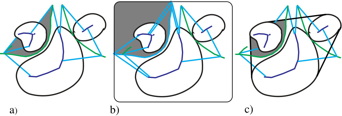 Figure 1
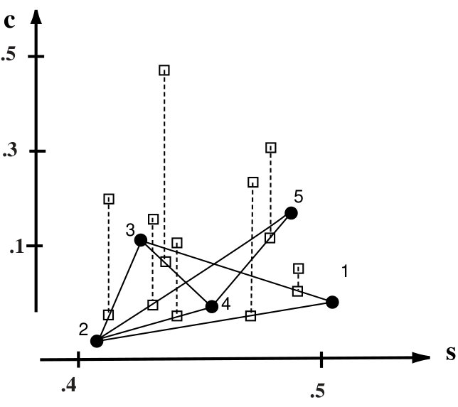 Figure 11
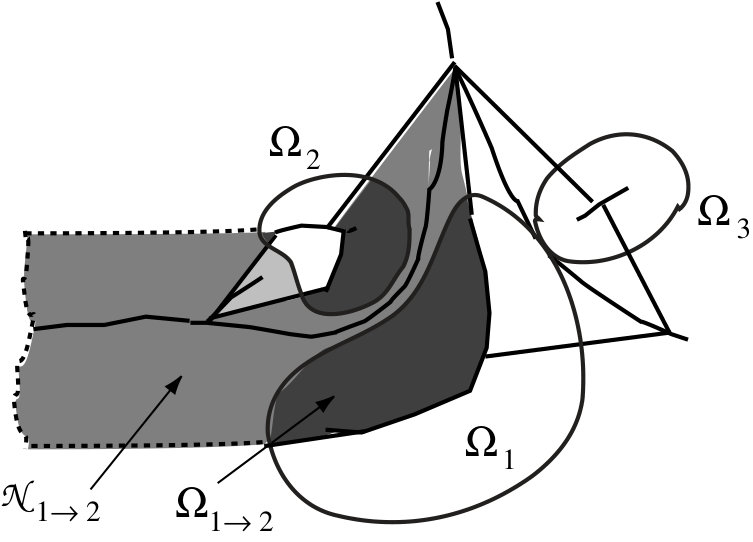 Figure 16
 Figure 16
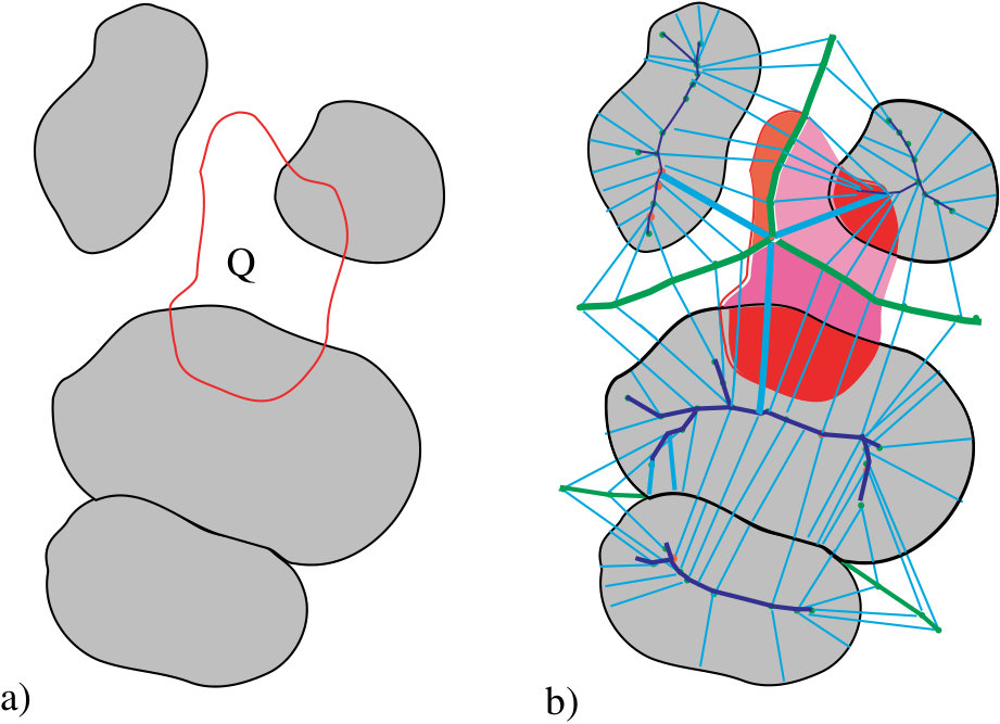 Figure 5
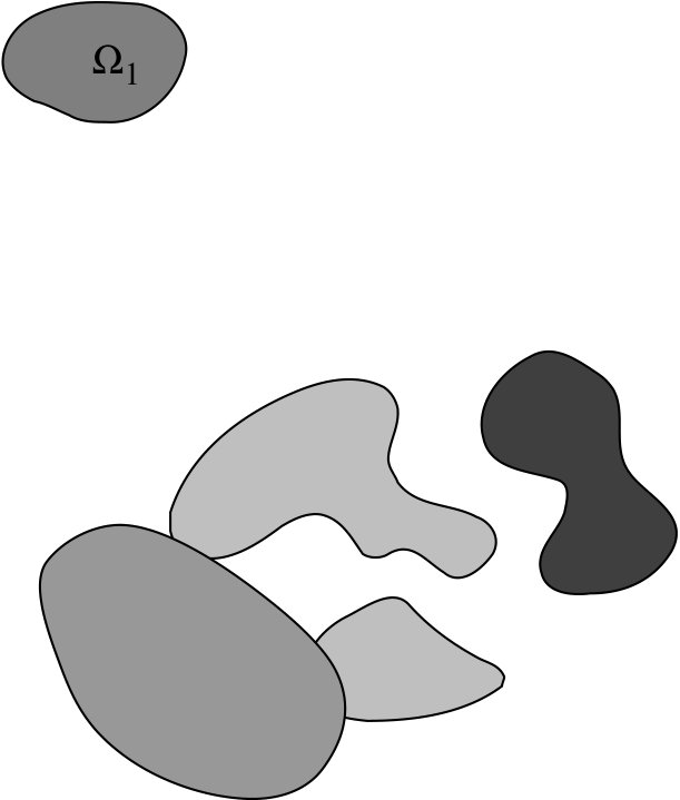 Figure 6
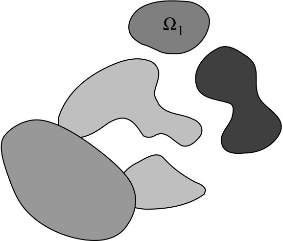 Figure 7
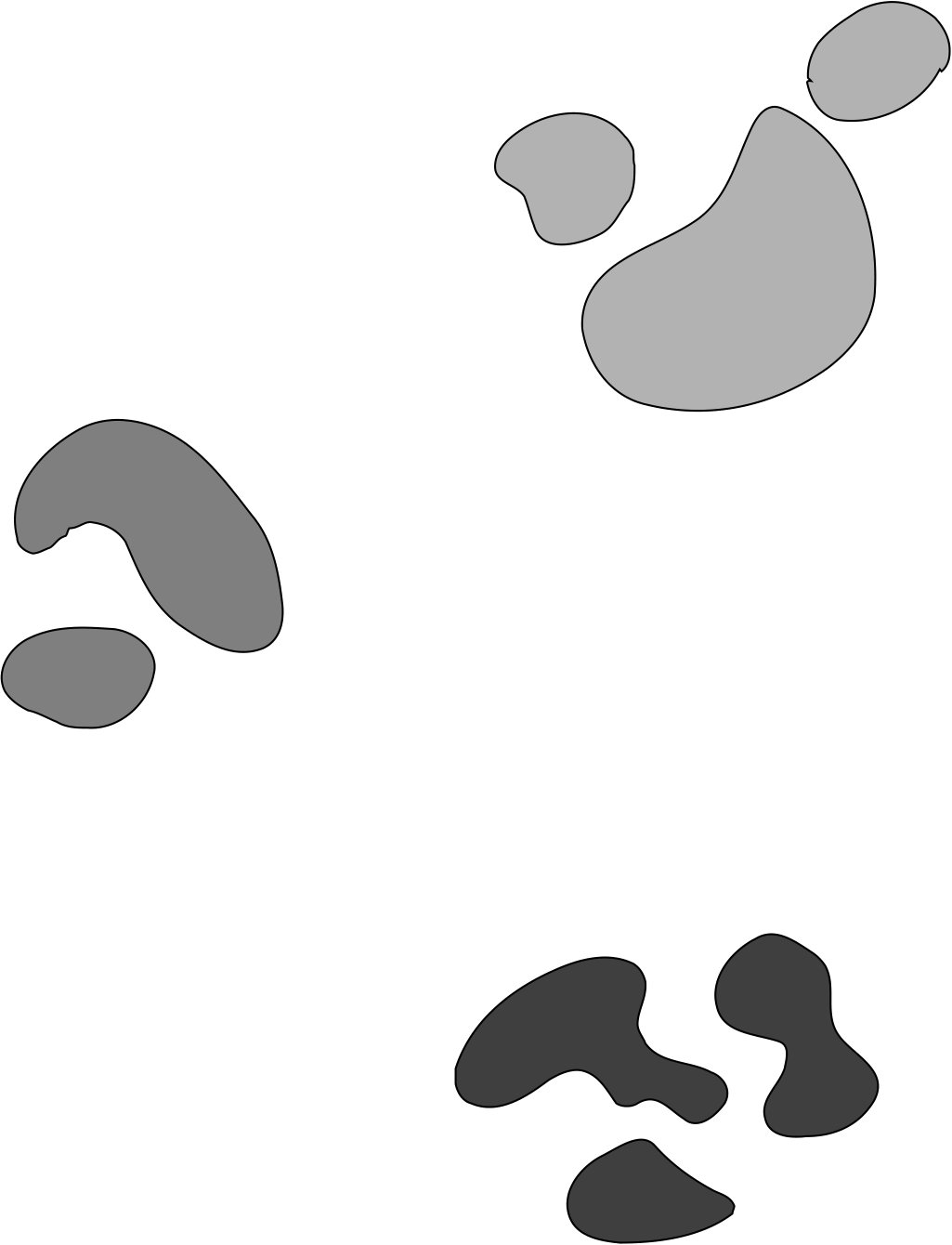 Figure 8
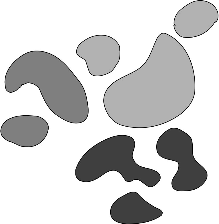 Figure 9
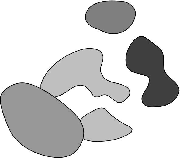 Figure 10
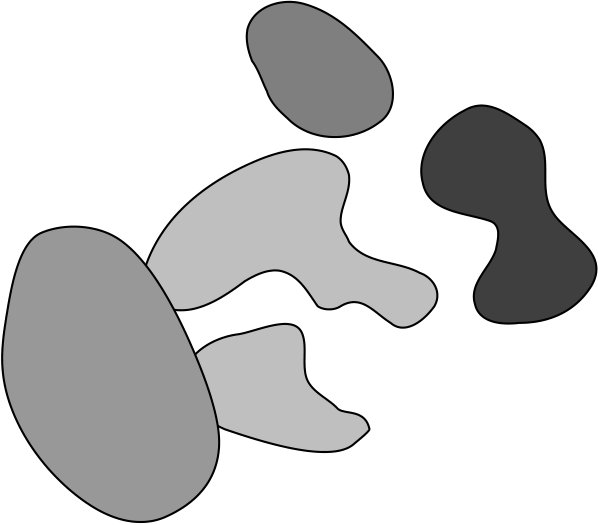 Figure 11
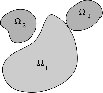 Figure 12
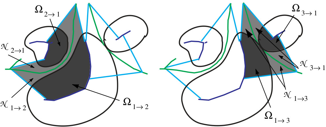 Figure 13
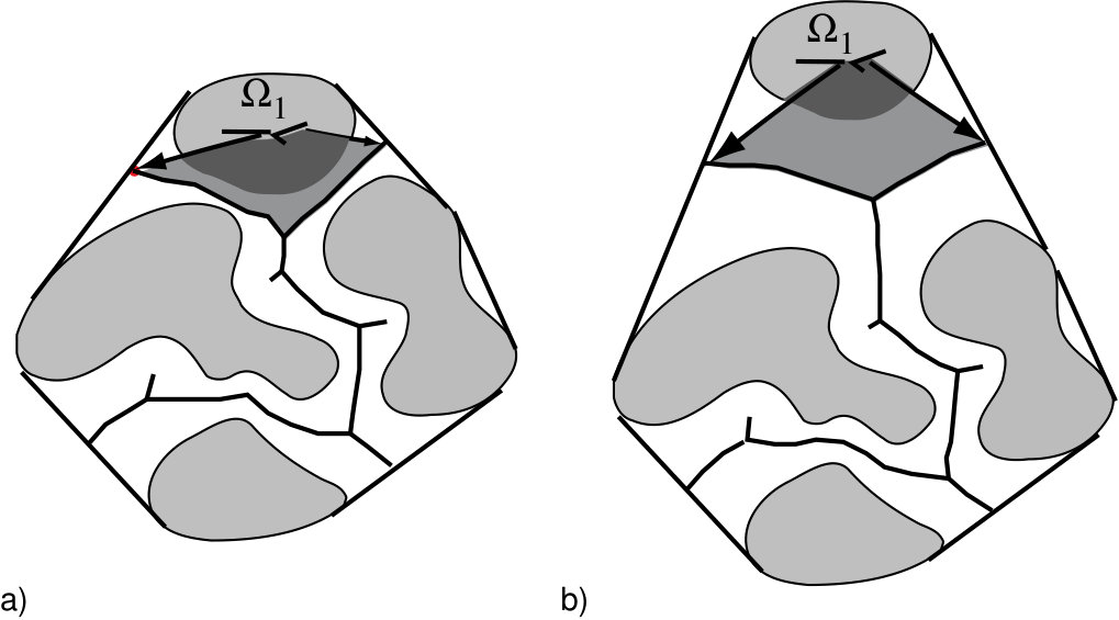 Figure 14
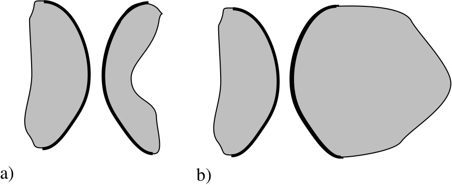 Figure 15
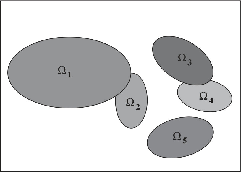 Figure 1
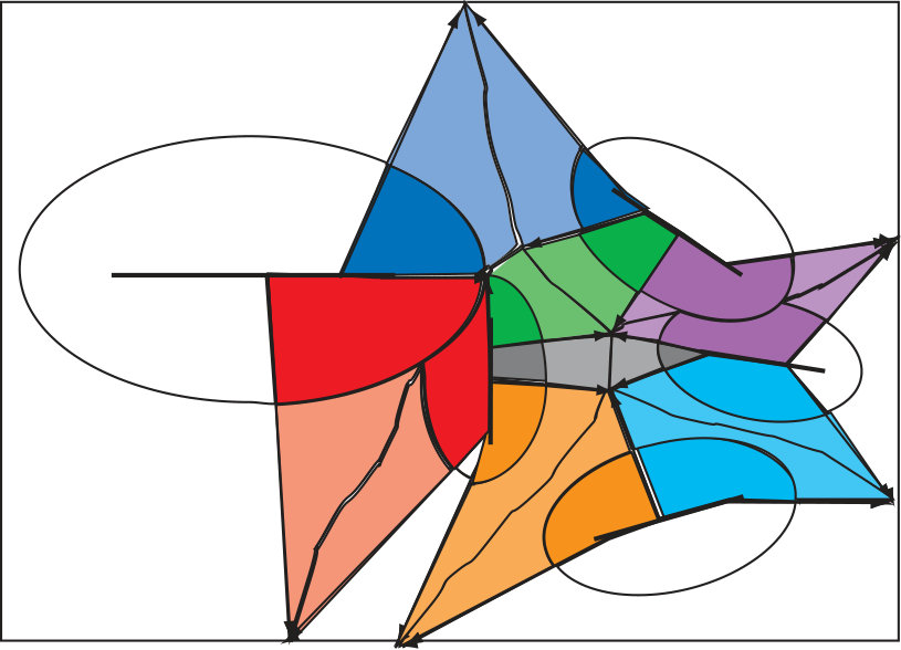 Figure 2
Peer Reviews
No public reviews on file for this paper yet. If you reviewed it on a platform where reviews are public (OpenReview, ICLR, NeurIPS, ICML), you can paste yours below so the community can read it here.
Videos
No videos yet. Explain this paper in a talk, walkthrough, or lecture? Add one.
Taxonomy
TopicsMedical Image Segmentation Techniques · Digital Image Processing Techniques · 3D Shape Modeling and Analysis
Shape and Positional Geometry of
Multi-Object Configurations
James Damon1 and Ellen Gasparovic2
Dept. of Mathematics
University of North Carolina
Chapel Hill, NC 27599-3250
Dept. of Mathematics
Union College
Schenectady, NY 12308
Abstract.
In [9], we introduced a method for modeling a configuration of objects in 2D and 3D images using a mathematical “medial/skeletal linking structure.” In this paper, we show how these structures allow us to capture positional properties of a multi-object configuration in addition to the shape properties of the individual objects. In particular, we introduce numerical invariants for positional properties which measure the closeness of neighboring objects, including identifying the parts of the objects which are close, and the “relative significance” of objects compared with the other objects in the configuration. Using these numerical measures, we introduce a hierarchical ordering and relations between the individual objects, and quantitative criteria for identifying subconfigurations. In addition, the invariants provide a “proximity matrix” which yields a unique set of weightings measuring overall proximity of objects in the configuration. Furthermore, we show that these invariants, which are volumetrically defined and involve external regions, may be computed via integral formulas in terms of “skeletal linking integrals” defined on the internal skeletal structures of the objects.
Key words and phrases:
Blum medial axis, skeletal structures, spherical axis, Whitney stratified sets, medial and skeletal linking structures, generic linking properties, model configurations, radial flow, linking flow, measures of closeness, measures of significance, proximity matrix, proximity weights, tiered linking graph
1991 Mathematics Subject Classification:
Primary: 53A07, 58A35, Secondary: 68U05
(1) Partially supported by the Simons Foundation grant 230298, the National Science Foundation grant DMS-1105470 and DARPA grant HR0011-09-1-0055. (2) This paper contains work from this author’s Ph. D. dissertation at Univ. of North Carolina.
1. Introduction
In many 2D and 3D images, such as medical images, there appears a configuration of objects, and the analysis of objects in the image benefits from modeling the interplay of the different objects’ shapes and their relative positions. First steps for such an approach for medical images was begun by the MIDAG group at UNC led by Pizer, see e.g. [16], [18], [15], [14], and [2]. These results use a modification of the classical Blum medial axis to model the individual regions together with user chosen, somewhat ad hoc, approaches to relating neighboring objects. Results for the Blum medial axis of an individual region, introduced by Blum-Nagel [1], have concerned its generic structure using a number of different approaches (see, e.g., Mather [19], Yomdin [27], Kimia et al [17], Giblin and Kimia [11], [12]), and its computation (see, e.g., for “grassfire flow” Siddiqi et al. [25], the surveys by Pizer et al. [22] and [24] including Voronoi methods, and for b-splines, Musuvathy et al. [21]). The modification uses methods from “skeletal structure”models for objects as single regions with smooth boundaries (for 2D and 3D see [5] or [7] and more generally [3], [4]). These results add considerable flexibility and stability to the classical Blum medial axis.
In [9] we introduced for configurations of objects in or medial/skeletal linking structures which capture both the shapes of the individual objects and their relative positions in the configuration. In this paper we develop an approach to the “positional geometry” of a configuration using mathematical tools defined in terms of the linking structure, which build upon the methods already developed for skeletal structures for single regions. Moreover, we will see that certain constructions and operators defined for skeletal structures and used for determining the geometry of individual objects can be extended to give simultaneously the positional geometric properties of the entire configuration. As such this provides a natural progression from individual objects to configurations of objects.
Given a collection of configurations, we may ask what are the statistically meaningful shared geometric properties of the collection of configurations, and how the geometric properties of a particular configuration differ from those for the collection. To provide quantitative measures for these properties, we will directly associate geometric invariants to a configuration. Such invariants may be globally defined depending on the entire configuration or locally defined invariants depending on local subconfigurations associated to each object.
For example, if we view the union of the objects as a topological space, then we can measure the Gromov-Hausdorff distance between two such configurations. We may also use the geodesic distance between the two configurations measured in a group of global diffeomorphisms mapping one configuration to another. Such invariants give a single numerical global measure of differences between two configurations. Instead, we will use skeletal linking structures associated to the configurations to directly associate both global and local geometric invariants which can be used to measure the differences between a number of different features of configurations in a variety of different ways.
In introducing these invariants, we will be guided by several key considerations. The first involves distinguishing between the differences in the shapes of individual objects versus their positional differences and how each of these contributes to the differences in the configurations, as illustrated in Figure 1. A first question for objects that do not touch is when they should be considered “neighbors”and what should be the criterion? Second, in measuring the relative positions of neighboring objects, more than just the minimum distance between their boundaries is required; we also wish to measure how much of the regions are close, see, e.g., Figure 2. A goal is then to define numerical measures of closeness of objects which takes into account both aspects.
Third, we seek a measure to distinguish how significant are objects within the configuration and to identify those that are mainly outliers. This would provide for a configuration a hierarchical structure for the objects, indicating which objects are most central to the configuration and which are less positionally significant. For example, in Figure 3, the position of object makes it more important for the overall configuration in b) than in a), where it is more of an “outlier.” A small movement of in a) would be less noticeable and have a smaller effect to the overall configuration than in b). By having a smaller effect we mean that the deformed configuration could be mapped to the original by a diffeomorphism which has smaller local distortions near the configuration in the case of a) versus b). Finally, there is the question of whether there are numerical invariants which can be used to determine when there are identifiable subconfigurations. An example of this is seen in Figure 4.
In Sections 2 and 3 we consider the “linking flow”associated to the linking structure. The nonsingularity of the linking flow is guaranteed in §2 by “linking curvature conditions” on the linking functions, given in a form which extends that given in [3, Thm 2.5] for the radial flow. Next, in §3, we use this linking flow to identify both the internal regions of neighboring objects and external regions shared by them, which are the “linking neighborhoods” between objects. Then, in §4, we show how to compute integrals over the boundaries of the objects or over general regions inside or outside the objects as “medial and skeletal linking integrals,”which are integrals defined on the skeletal sets in the interiors of the objects. Lastly, in §5, we introduce and compute several “volumetric–based” numerical invariants that include measures of the relative closeness of neighboring objects and relative significance of the individual objects. We furthermore show how they may be computed from the medial/skeletal linking structure via skeletal linking integrals.
Then, in §6 we will combine the invariants which measure these geometric features in two different ways. One is to construct a “proximity matrix”which captures the closeness of all objects in the configuration and to which the Perron-Frobenius theorem can be applied, yielding a unique set of “proximity weights”assigned to the objects, measuring their overall closeness in the configuration. The second is to construct a “tiered graph structure,” which is a graph with vertices representing the objects, edges between vertices of neighboring objects, and values of significance assigned to the vertices, and closeness assigned to the edges. Then, as thresholds for closeness and significance vary, the resulting subgraph satisfying the conditions will exhibit the central objects (and outliers) of the configuration, various subgroupings of objects and a hierarchical ordering of the relations between objects. The skeletal linking structure also allows for the comparison and statistical analysis of collections of objects in and , extending the analyses given in earlier work for single objects.
2. Linking Flow and Curvature Conditions
We model a configuration of objects in 2D or 3D images by a collection of regions in either or , with each modeling one of the objects, whose boundaries may share common boundary regions (see e.g. [9, Fig. 1 and 2]) and along their edges there are singularities of generic type corresponding to whether the objects are flexible or rigid (see e.g. [9, Fig. 5 and 6]).
Medial/Skeletal Linking Structures
We recall from [9] the definition of a skeletal linking structure for the multi-object configuration . First of all, it consists of skeletal structures for each , where each is a stratified set in and is a multi-valued vector field on whose vectors end at boundary points in (see[5] for 2D or 3D regions, or more generally [4]). By being a stratified set we mean for regions in it is a disjoint collection of smooth curve segments ending at branching or end points, and for , it is a disjoint collection of smooth surface regions, curve segments and points, with the surfaces ending at the curves and points. We may define a stratified set from by replacing points by pairs , where varies over the multiple values of at , with strata formed from strata of together with a choice of smoothly varying values for . The mapping sending sends the strata to strata of . This has the benefit of being able to consider multi-valued objects on as single-valued objects on .
We express , where are multi-valued unit vector fields on . In addition, the are multi-valued “linking functions”defined on , and there are then defined the multi-valued “linking vector fields” on each . These become single valued on .
There are additional conditions of [9, Def. 3.2] to be satisfied for to be the skeletal linking structure for . Conditions S1 - S3 concern a refinement of the stratification of and the differentiability properties of on the strata of the refinement. Also, the conditions L1 - L4 concern the relations between the linking vector fields from different objects and the nonsingularity of the “linking flows” generated by the linking vector fields. Regions defined by the linking flows are what we use to identify properties of the positional geometry of the configuration.
Nonsingularity of the Linking Flow
The nonsingularity of the radial flow, which occurs within the regions, was established in [3, §4] (and see [5, §2]) using the radial and edge shape operators and , which are multi-valued operators defined on , with defined at all points except the edge points of and defined at these points. These capture the geometric properties of the radial vector field and play an important role in determining the local geometric properties of the boundary and the relative and global geometric properties of the region (see [4] and [5, §3, 4]). Although their properties differ from those of the differential geometric shape operators appearing in differential geometry, their eigenvalues , the principal radial curvatures and generalized eigenvalues , the principal edge curvatures, play an equally important role.
We next explain how they appear in the sufficient conditions we give for nonsingularity of the linking flow. As well we give formulas for the evolution of the radial and edge shape operators under the linking flow.
Recall [9, (3.1)], the linking flow from is defined by
[TABLE]
where ranges over all possible values and
[TABLE]
For , this flow is the radial flow at twice the speed and it extends the radial flow to the exterior of the regions for and ends at the “linking axis”. We let for each and refer to as the linking mapping from strata of the refinement of to strata of the linking axis. We refer to the combined union of the for all by .
To establish the conditions for the nonsingularity of the linking flow for the skeletal linking structure , we introduce the following two conditions:
- (1)
(Linking Curvature Condition ) For all points and all values ,
[TABLE]
for all positive principal radial curvatures ; 2. (2)
(Linking Edge Condition ) For all points (the closure of ),
[TABLE]
for all positive principal edge curvatures .
In these conditions, the values of and either or are at the same point and for the same value of .
The nonsingularity of the linking flow (and the radial flow) for a skeletal linking structure is given by the following.
Theorem 2.1** (Nonsingularity of the Linking Flow).**
Let be a skeletal linking structure in or which satisfies: the Linking Curvature Conditions and Linking Edge Conditions on all of the strata of all . Then, the radial flow also satisfies the radial curvature and edge curvature conditions on each stratum. Hence, the following properties hold.
- i)
On each stratum of the refinement of , the linking flow is nonsingular and remains transverse to the radial lines.
- ii)
Hence, the image of the linking map on is locally a smooth stratum of the same dimension and which may only have nonlocal intersections from distant points in . If there are no nonlocal intersections then is a smooth stratum.
- iii)
The image of a stratum of under the radial map is a smooth stratum of of the same dimension.
- iv)
For both flows, at points of the top dimensional strata, the backward projection along the lines of will locally map strata of , resp. , diffeomorphically onto the smooth part of .
- v)
Thus, if there are no nonlocal intersections, each will be a piecewise smooth embedded surface.
The proof of this theorem follows from Proposition 8.1 in [8] and its corollaries along with Theorem 2.5 of [5]; see also [10, Chap. 6].
Evolution of the Shape Operators Under the Linking Flow
We may translate the vectors along the lines of each to the level sets of the linking flow. We may use these translated vectors as a radial vector field on the level set. Hence, for each we may define corresponding radial shape operators on the level sets (curves or surfaces) in a neighborhood of . We can best relate them to the radial or edge shape operators on in terms of their matrix reprsentations. For and each choice of , there is a smooth stratum of containing in its closure and which smoothly extends through and a smoothly varying value of defined in a neighborhood of extending . We denote the tangent space to this stratum at by . For we choose a basis for , which is either a single vector for configurations in , or for . We then let denote the image of under which is a basis for the tangent space to the level set at . At points for , instead a nonzero vector is completed to a basis using for the source and the unit normal vector to for the target. We denote the resulting matrix representation of by ; but for , it evolves to also become radial shape operators ; and we use a basis , which is the image of the basis of under with adjoined.
Remark 2.2**.**
In the 3D case and are matrices; while in the 2D case, is a matrix formed from the single radial curvature (see e.g. Examples 2.3 and 2.4 in [5]).
Then, the evolved radial shape operators under the linking flow are given by the following.
Proposition 2.3** (Evolution of the Shape Operators).**
Suppose with value (with a smooth value of in a neighborhood of ). Provided the following conditions are satisfied, the linking flow is nonsingular and the evolved radial shape operator on the level surface in a neighborhood of is given by the following.
For , if is not an eigenvalue of for , then
[TABLE]
- 2)
For , if is not a generalized eigenvalue of for , then
[TABLE]
The derivation of these results can be found in [8, §7] and [10, Chap. 6] extending the results in [4], or see [5, §2].
Shape Operators on the Boundary and Linking Medial
Axis
As a consequence of the corollaries, we can deduce the shape operator for the linking axis , and in a region where the partial Blum condition is satisfied, the differential geometric shape operator on the boundary. First, for the boundary, it is reached at . If for the radial vector field is orthogonal to at the point , then we say that the skeletal structure satisfies the partial Blum condition at . If it satisfies the partial Blum condition in a neighborhood of a smooth point of , then in Proposition 2.3 gives the differential geometric shape operator for at , and hence completely describes the local geometry of the boundary at . This result and its consequences follow from [4, §3] and also see [5, §3].
If instead we consider the image of under the linking flow, then to such a point there is the corresponding point . We then have a value of a radial vector field at , with , , and associated to the value . This vector at the point ends at . This defines a multi-valued vector field on . Thus, we can view as a skeletal structure for the exterior region. We can determine the corresponding radial or edge shape operator at by the following (see [8, Cor. 8.7]).
Corollary 2.4**.**
If is as in the above discussion, then the radial shape operator for the skeletal structure at is given by either: if is a non-edge closure point, then with the notation of Proposition 2.3,
[TABLE]
or if is an edge closure point, then
[TABLE]
This follows because the associated unit vector field at is . Thus, the radial shape operator for at is the negative of that for the stratum of , viewed as a level set of the linking flow from . Hence, by Proposition 2.3 we obtain the result.
3. Positional Properties of Regions Defined Using the Linking Flow
We next consider how the medial/skeletal linking structure for a multi-object configuration in or allows us to introduce numerical measures capturing various aspects of the object’s positions within the configuration. There are two possibilities for this. One is to base the numerical quantities on geometric properties of the boundaries of the objects. The second is to use instead volumetric measures for subregions of the objects and identified regions in the external complement which capture positional information about the objects.
The problem with the first choice is that two regions may show the same boundary region to each other even though there are other pairs of regions showing the same boundaries to each other but which may have completely different shapes and volumes, as shown in Figure 5. The alternative is to keep track of the relation between all points of all boundaries of each pair of regions. However, this involves an enormous redundancy in the data structure. The skeletal linking structure avoids this redundancy, allowing additional geometric information to be computed directly from the linking structure. We also shall see in §4 that for general skeletal linking structures, using volumetric measures to capture positional information will allow us to express these numerical quantities as integrals over the internal skeletal sets of appropriate mathematical quantities derived from the linking structure .
Because finite volumetric measures will require bounded regions in the complement, we will first consider regions defined in the unbounded case and then introduce bounded versions.
Medial/Skeletal Linking Structures in the Unbounded Case
We begin by considering regions and modeling objects in the configuration that are linked via the linking structure and identifying regions using the linking flow on each . We recall in [9] that and are said to be “linked” if there are strata in and in which map to the same stratum in under the linking flow. We then introduce the following regions as illustrated in Figure 6.
Regions Defined by the Linking Flow:
- i)
will denote the union of the strata of which are linked to strata of , and we refer to it as the strata where is linked to (the strata being in indicate on which “side”of the linking occurs).
- ii)
denotes the region of linked to .
- iii)
denotes the linking neighborhood of linked to .
- iv)
is the boundary region of linked to .
- v)
, is the total region for linked to .
Then, we make a few simple observations. First, will consist of the strata of the linking axis where the linking between and occurs; and second, the regions for a fixed but different may intersect on the images under the linking flow of strata where there is linking between and two or more other objects.
Next, strata of may involve “self-linking,” which means different strata of may be linked to each other (see e.g. [9, Fig. 9]). We will still use the notation , , etc. for the strata, regions etc. involving self-linking. Then, will intersect on strata where “partial linking” occurs.
Finally the remaining strata in lie in , which is introduced in [9] and consists of the union of strata which are unlinked. By property in [9, Def. 3.2], the radial flow from the union of the defines a diffeomorphic parametrization of the complement of the regions reached by the linking flow. We may flow at twice the radial flow speed to agree with the linking flow on the rest of . We still refer to this completed flow as the linking flow, and then denote the corresponding regions for by: , , and .
Then, we have the decompositions
[TABLE]
with
[TABLE]
but the various and/or may have non-empty intersections, as explained above. There are analogous decompositions for and . Also, we denote the total linking neighborhood by . Then, is the total neighborhood of (in the complement of the configuration), whose interior consists of points external to the configuration which are closest to .
We let denote the portion of the boundary that is not shared with any other region. We recall that on the strata of corresponding to those in , the linking flow is constant in for . Hence, at these points only consists of boundary points of . Off of these points we can describe the structure of using the linking flow. We summarize the consequences of the properties of the linking flow (see [8, Cor. 9.2]).
Corollary 3.1**.**
For a multi-object configuration with skeletal linking structure , there are the following parametrizations for each region associated to by the portions of the level sets of the linking flow in those regions:
* is parametrized by the level sets of the linking flow for ;*
- 2)
* is parametrized by the level sets of the linking flow for ;*
- 3)
* is parametrized by the level sets of the linking flow for ; and*
- 4)
* is parametrized by the level sets of the radial flow for .*
Medial/Skeletal Linking Structures for the Bounded Case
As we have mentioned, because the regions are often unbounded, there is no meaningful numerical measure of their sizes. We can overcome this problem for practical considerations by introducing a bounded region containing the configuration and such that its boundary is transverse both to the stratification of and to the linking vectors on . In [9], we describe a number of different possibilities for obtaining bounded regions including: a bounding box or bounding convex region, the convex hull of the configuration, a natural or intrinsic bounding region, or a region defined by a user-specified threshold for linking, see, e.g., Figure 8.
Then, we can either truncate the linking vector field, or define it on all of for all by defining it on and subsequently refining the stratification so that the linking vector field ends at on appropriate strata. This maintains the nonsingularity of the linking flow as we are merely either reducing or defining on .
Thus, we have the corresponding properties from Corollary 3.1, except that for properties 2), 3), and 4) the linking flow and corresponding regions , , and may only extend to . These regions, which are now compact, are obtained from the unbounded regions by intersecting them with . We refer to this as the bounded case, referring the reader [9, §3] for more details. Moreover, we still obtain analogous formulas for the evolution of the radial shape operators for those level sets of the linking flow while they remain within .
Relevance of the Linking Regions for Positional Geometry
The regions capture various aspects of the positional geometric properties of the configuration. Two regions and are neighbors if the regions , , , etc are nonempty, as are the corresponding , etc. Then, the and represent the boundary regions “between”these neighbors. Moreover, the and represent the internal portions of the regions which are “closest”to the neighbors. These can be compared to the linking neighborhoods and to see how close the neighbors are. The larger the linking neighborhoods are compared to the internal neighboring regions the further away are the neighboring regions. If one region has large linking neighborhoods relative to all of its neighbors, then it plays a less significant positional role for the configuration. This perspective will lead us in §5 to introduce volumetric invariants of these regions which capture this positional geometry. Before doing so, we next explain how numerical volumetric invariants can be obtained from the linking structures using “linking integrals”on the skeletal sets of the regions.
4. Global Geometry via Medial and Skeletal Linking Integrals
We now will use the associated regions we have introduced for a configuration via a skeletal linking structure to define quantitative invariants measuring positional geometry for the configuration. We will do so in terms of integrals which are defined on the internal skeletal sets. We begin by defining these integrals, and then we give a number of formulas for integrals of functions on the regions or boundaries of the configuration in terms of these integrals on the internal skeletal sets (see [8, §10] and for 2D and 3D single regions [7, §3.4]).
In practice, skeletal structures have been modeled discretely, as can be skeletal linking structures. For these the integrals then can be discretely approximated from the linking structure to compute the appropriate numerical invariants.
Defining Medial and Skeletal Linking Integrals
We begin by considering a medial or skeletal linking structure for the configuration in or . We again let denote the disjoint union of the for each region for . Each has its double , so we introduce the double for the configuration by . For each , there is a canonical finite-to-one projection , mapping . The union of these defines a canonical projection , such that for each .
We will define the skeletal integral on for a multi-valued function , by which we mean for any , may have a different value for each different value of at . Such a pulls-back via to a well-defined map so that .
We recall that by Proposition 3.2 of [6], for each , there is a positive Borel measure on , which we call the medial measure. If we let , , denote the inverse images of under the canonical projection map , then each is a copy of , representing “one side of ” with the smoothly varying value of associated to the copy. For each copy we let . Here denotes the Riemannian length or area on , as , resp. . Also, where is a value of the unit vector field corresponding to the smooth value of for and is the normal unit vector pointing on the same side as .
Then, the integral of the multi-valued function over is, by definition, the sum of the integrals of the corresponding values of over each copy with respect to the medial measure . It is shown in [6] that for continuous , this gives a well-defined integral and this extends to integrals of “Borel measurable functions” on , which include piecewise continuous functions. Then, these distinct medial measures on together define a medial measure on ; and the integral of a Borel measurable multi-valued function on is defined to be
[TABLE]
where each integral on the RHS is the integral of over with respect to the measure , and it can be viewed as an integral of over “both sides of .”. If the integral is finite then we say the function is “integrable”.
We refer to the integrals in (4.1) as medial or skeletal linking integrals, depending on whether the linking structure is a Blum medial linking structure or a skeletal linking structure.
Computing Boundary Integrals via Medial Linking Integrals
We now show how, for a multi-object configuration with “full” Blum linking structure, we may express integrals of functions on the combined boundary as medial integrals. We emphasize that the full Blum linking structure allows the Blum medial axis to extend up to the edge-corner points of the boundaries. This does not alter the existence nor definition of the integrals, see [8, §10].
First, we consider a Borel measurable and integrable function which is multi-valued in the sense that for any -edge-corner point , may take distinct values for each region , , containing on its boundary. Thus, if denotes the shared boundary region of and , may take different values on and . For example, and may have different boundary properties such as densities measured by .
By the integral of such a multi-valued function over we mean
[TABLE]
where denotes the values of on for and denotes the Riemannian length (for 2D) or area (for 3D) for each .
Then, for the radial flow map , we define by , where the value on is the value associated to . Then, is a multi-valued Borel measurable function on . We may compute the integral of over by the following result [8, Thm 10.1].
Theorem 4.1**.**
Let be a multi-object configuration with (full) Blum linking structure. If is a multi-valued Borel measurable and integrable function, then
[TABLE]
where is the radius function of each .
In the case of a skeletal structure, there is a form of Theorem 4.1 which still applies. For each region , with , let denote a Borel measurable region of which under the radial flow maps to a Borel measurable region of . Let and . We suppose that the skeletal structure satisfies the “partial Blum condition” on , by which we mean: for each , the compatibility -form vanishes on (recall this means that the radial vector at points of is orthogonal to at the point where it meets the boundary). Note that for a skeletal structure this forces to be contained in the complement of .
Then, there is the following analogue of Theorem 4.1.
Corollary 4.2**.**
Let be a multi-object configuration with skeletal linking structure which satisfies the partial Blum condition on the region , with image under . If is a multi-valued Borel measurable and integrable function, then
[TABLE]
Remark 4.3**.**
One may compute the length (2D) or area (3D) of by choosing in Theorem 4.1. There is an analogous result for a region which is the image of a region under the radial flow. If the configuration is modeled by a skeletal linking structure which satisfies the partial Blum condition on , then the length, resp. area, of is given by .
Computing Integrals over Regions as Skeletal Linking
Integrals
Next, we turn to the problem of computing integrals over regions which may be partially or completely in the external region of the configuration. Quite generally we consider a Borel measurable and integrable scalar-valued function defined on or , but only nonzero on a compact region. We shall see that we can compute the integral of as an integral of an appropriate related function on the internal skeletal sets.
Since we are in the unbounded case, we first modify the skeletal linking structure by defining on to be . The linking flow on is a diffeomorphism for , see [8, Prop. 14.11].
Next, we replace the linking flow by a simpler elementary linking flow defined by , for (or if ). The elementary linking flow is again along the radial lines determined by ; however, the rate differs from that for the usual linking flow. This means that the level surfaces will differ, although the images of strata under the elementary linking flow agree with that for the linking flow. In addition, as the linking flow is nonsingular, the linking curvature and edge conditions are satisfied. Then, viewing the linking vector field as a radial vector field, the radial curvature and edge curvature conditions are satisfied, and hence imply the nonsingularity of the elementary linking flow.
Then, using the elementary linking flow, we can compute the integral of as a skeletal linking integral. We define a multi-valued function on as follows: for with associated smooth value and linking vector in the same direction as (so ),
[TABLE]
provided the integral is defined. Then, we have the following formula for the integral of as a skeletal linking integral [8, Thm 10.6].
Theorem 4.4**.**
Let be a multi-object configuration in or with a skeletal linking structure. If is a Borel measurable and integrable function which is zero off a compact region, then is defined for almost all , it is integrable on , and
[TABLE]
Remark 4.5**.**
If we compare this formula with that given for a single region in Theorem 6.1 of [6], we notice they have a slightly different form in that a factor of appears to be missing . However, as noted in Remark 6.2 of that paper, it is possible to use a change of coordinates to rewrite
[TABLE]
so that the form of (4.6) agrees with the form given in [6]. The apparent difference in form will also appear in all of the following formulas compared with the corresponding ones in [6].
Reducing to Integrals for Bounded Skeletal Linking
Structures
We may replace the unbounded skeletal structure by a bounded one and replace the integrals by integrals over bounded regions. If is zero off the compact region , then we may find a compact convex region with smooth boundary containing both the configuration and . Then, we can modify the linking structure by reducing the so it is truncated where it meets , the boundary of , and defining on as the extensions of the radial vectors to where they meet . Because the extended radial lines are transverse to , the new smaller values of remain differentiable on the strata of each . Still letting the denote the new smaller values, the corresponding truncated vector fields will still be denoted by . Then the formula for the integral of is still given by (4.5). We shall assume we have chosen a bounded linking structure for the remainder of this section.
To simplify the statements for the remainder of this section, we shall use the notation for a region or : for or for .
For each , we let
[TABLE]
We can view as a weighted -dimensional measure of the length of the intersection of with the linking line from determined by . Then, applying Theorem 4.4 in the special case where , we obtain an analogue of Crofton’s formula giving the area, resp. volume, of as a skeletal integral of using [8, Cor. 10.9].
Corollary 4.6** (Crofton Type Formula).**
Let be a multi-object configuration with skeletal linking structure in for , or . Suppose is a compact subset. Then
[TABLE]
Decomposition of a Global Integral using the Linking
Flow
We next decompose the integral on the RHS of (4.5) into internal and external parts using the alternative integral representation of using the linking flow. We do so by applying the change of variables formula to relate the elementary linking flow with the linking flow , both of which flow along the linking lines but at different linear rates.
We define
[TABLE]
Then, we may decompose as follows, [8, Cor. 10.10].
Corollary 4.7**.**
Let be a multi-object configuration in or with a skeletal linking structure. If is a Borel measurable and integrable function for , resp. , which equals [math] off a compact set, then and are defined for almost all , they are integrable on , and
[TABLE]
where
[TABLE]
with an analogous formula with replaced by everywhere in (4.11).
The first integral on the RHS of (4.10) is the “interior integral” of within the configuration using the radial flow, and the second integral is the“external integral” computed using the linking flow outside of the configuration. Then we may further decompose each of these integrals using (4.11) into integrals over the distinct linking regions as illustrated in Figure 7.
Skeletal Linking Integral Formulas for Global Invariants
We now express the areas (2D) or volumes (3D) of regions associated to the linking structure, which we introduced in §3, as skeletal linking integrals. We may apply the same reasoning as in Corollary 4.6, using Corollary 4.7 to compute the volume of a compact 2D or 3D region as a sum of internal and external integrals.
For these calculations we will use the polynomial expression in
[TABLE]
In the 2D case, ; and in the 3D case, , where and , for the principal radial curvatures.
Areas and Volumes of Linking Regions as Skeletal
Integrals
Then, we can express the areas or volumes of various linking regions as integrals of for various choices of .
Corollary 4.8**.**
Let be a multi-object configuration with a bounded skeletal linking structure in for , resp. . Then, the areas, resp. volumes, of linking regions in are given by the following:
[TABLE]
As well as these formulas, we can compute the volumetric invariants of other linking regions such as , , etc. using skeletal linking integrals of the polynomials or . For example,
[TABLE]
with an analogous formula for .
As a consequence, we obtain generalizations of the classical formula of Weyl for “volumes of tubes”and Steiner’s formula for volumes of “annular regions”.
Corollary 4.9** (Generalized Weyl’s Formula).**
Let , for or , be a multi-object configuration with a bounded skeletal linking structure. Then,
[TABLE]
The sense in which this generalizes Weyl’s formula is explained for the case of a single region with smooth boundary in [6, §6, 7]. For Steiner’s formula, we note that as explained in §3, represents the total neighborhood of , which is the region about extending along the linking lines. This is a generalization of an “annular neighborhood”about a region which depends on the specific type of bounding region (see Figure 8).
Corollary 4.10** (Generalized Steiner’s Formula).**
Let , for or be a multi-object configuration with a bounded skeletal linking structure. Then,
[TABLE]
Remark 4.11**.**
The regions in both generalizations of Weyl’s formula and Steiner’s formula for different and will only intersect in lower dimensional regions. Thus, in both cases we can sum the integrals on the RHS for multiple to obtain formulas for a union of .
5. Positional Properties of Multi-Object Configurations
In this section we define positional geometric invariants of configurations in terms of volumetric measures of associated regions defined by the linking structure. We emphasize that the volumetric measures versus boundary measures of positional geometry have two advantages: 1) they are computable from the skeletal linking structure, and unlike surface measures, they do not require the partial Blum condition to compute the invariants; and 2) as in Figure 5, the volumetric invariants capture the total geometric structure of regions better than boundary measures.
We proceed as follows. We first use the linking structure to determine which of the objects should be regarded as neighboring objects. Then, we use the regions associated to the linking structure to define invariants which measure the closeness of such neighboring objects. Second, we further introduce numerical invariants measuring the positional significance of objects for the configuration. These allow us to identify which objects are central to the configuration and which ones are peripheral.
In §6 we will use the closeness measures to construct a “proximity matrix”which yields proximity weights for the objects based on their closeness to other objects. We also will use both types of invariants to construct a tiered linking graph, with vertices representing the objects, and edges between vertices representing neighboring objects, with the closeness and significance values assigned to the edges, resp. vertices. By applying threshold values to this structure we can exhibit the subconfigurations within the given thresholds.
Neighboring Objects and Measures of Closeness
We consider a configuration , with a bounded skeletal linking structure. We use linking between objects and as a criterion for their being neighbors, so that objects which are not linked are not considered neighbors. The simplest measure of closeness between neighboring objects is the minimum distance between the objects. However, this ignores the size of the objects and how big a portion of each object is close to the other object, as illustrated in Figure 2 where is close to for a small region but is close to over a larger region. Moreover, if we choose a more global definition of closeness involving all neighboring boundary points, then as in Figure 5, this will not measure the portions of the objects which are close. We do overcome both of these issues by using volumetric measures of appropriate regions defined using the linking structures.
For a configuration with a skeletal linking structure, we introduced in §3 regions and which capture the neighbor relations between and . Since and share a common boundary region in , they are both empty if one is, and then both and are empty. In that case and are not linked. Otherwise, we may introduce a measure of closeness.
There are two different ways to do this, each having a probabilistic interpretation. First, we let
[TABLE]
Then, is the probability that a point chosen at random in will lie in (see Figure 9); so is the probability that a pair of points, one each in and both lie in the corresponding regions and .
Note that contains much more information than the closest distance between and , and even the “- measure”of the region between and . It compares this measure with how much of the regions and are closest as neighbors. If both and are empty, we let , , and . Also, we let . Thus, from the collection of values we can compare the closeness of any pair of regions.
Since these invariants depend on a bounded skeletal linking structure, one way to introduce a parametrized family is by considering the varying threshold values . For example, may represent the maximum allowable values for or the maximum value of relative to some intrinsic geometric linear invariant of . As increases, the bounded region increases and how varies indicates how the closeness of the regions varies when larger linking values are taken into account. Thus, this provides a method to use the local properties of the skeletal linking structure to introduce a scale of local closeness.
A second way to introduce a measure of closeness is to use an “additive contribution” from each region and define
[TABLE]
Here is the probability that a point chosen in the region lies in the configuration, i.e. in . We also let if and are not linked; and we let . Again, to obtain a more precise measure of closeness, we can vary a measure of threshold and obtain a varying family . The invariants satisfy . The value [math] indicates no linking, for values near [math], the regions are neighbors but distant so they are “weakly linked,”and for values close to , the regions are close over a large boundary region and are “strongly linked.”
There is a simple but crude relation between and the pair and :
[TABLE]
As , this is only useful when the two regions are weakly linked.
Measuring Positional Significance of Objects Via Linking
Structures
In order to measure positional significance of an object among a collection of objects, we can think in both absolute and relative terms. In each case, we emphasize that we are considering a form of geometric significance of objects relative to the configuration, rather than some other notion such as significance in the sense of statistics. We begin with the relative version. Given , we define the positional significance measure
[TABLE]
It takes values . For values near [math], the portion of the region of linked to other regions is a small fraction of the external region between and the other regions. Thus, compared to its size it is distant from other neighboring objects, so it is a peripheral region of the configuration. We would have the value if is not linked to any other region in , which may occur if there is a threshold for which the region is not linked to another region with a linking vector of length less than the threshold. By contrast, if is close to , then there is very little external region between and the other regions. Thus, is central for the configuration, see Figure 10. Note that
[TABLE]
so that being weakly linked to the other regions implies it has small significance for the configuration. If we would like to further base the positional significance of the region on its absolute size, we can alternatively use an absolute measure of positional significance defined by . Then, the effect of the smallness of will be partially counterbalanced by the size of .
Properties of Invariants for Closeness and Positional
Significance
We consider three properties of these invariants:
computation of all of the invariants as skeletal linking integrals;
- 2)
invariance under the action of the Euclidean group and scaling; and
- 3)
continuity of the invariants under small perturbations of generic configurations.
Computation of the Invariants as Skeletal Linking
Integrals
We can use the results from the previous section to compute as skeletal linking integrals the above volumes of regions associated to . This is summarized by the following, see [8, Thm. 11.3].
Theorem 5.1**.**
If , for or is a multi-object configuration, with a bounded skeletal linking structure, then all global invariants of the configuration which can be expressed as integrals over regions in , resp. , can be computed as skeletal linking integrals using Theorem 4.4. In particular, the invariants , , , and are given as the quotients of two skeletal linking integrals using (4.8) and (4.14).
Remark 5.2**.**
We emphasize that we could try to alternatively use boundary measures for the regions to define closeness and significance. There are two problems with this approach. From a computational point of view, the skeletal structures could only be used where the partial Blum condition is satisfied. Moreover, boundary measures do not capture how much of the regions are close to each other (only where their boundaries are close). For these reasons we have concentrated on (ratios of) volumetric measures to capture positional geometry of the configuration.
Invariance Under the Action of the Euclidean Group
and Scaling
Second, we establish the invariance of the invariants defining closeness and significance under Euclidean motions and scaling. Let , for or be a multi-object configuration, with a bounded skeletal linking structure . If is a Euclidean motion and is a scaling factor, then we may let , where and . We also let be a skeletal linking structure for defined by , , and . As preserves distance and angles, we have , and the image of the linking flow for is the linking flow for . Then, satisfies the conditions for being a skeletal linking structure for . As , the corresponding bounded linking structure for using is the image of that for for . Then, the associated linking regions for are the images of the corresponding associated linking regons for . Since preserves volumes, the invariants for closeness and significance are preserved by .
If instead we consider a scaling by the factor , then we let . Now the images of and under define a configuration in . We likewise let be defined by , , and (and ). As before this is a skeletal structure for . Everything goes through except that multiplies volume by . However, as the invariants are ratios of volumes, they again do not change. We summarize this with the following.
Proposition 5.3**.**
If , for or is a multi-object configuration, with a skeletal linking structure, then the invariants , , , and are invariant under the action of Euclidean motion and scaling applied to both and for the image of the skeletal linking structure for the image configuration and bounding region.
We note that if we consider the absolute significance , then it is still invariant under Euclidean motions. However, under scaling by , it changes by the factor for ; but this would not alter the hierarchy based on absolute significance, as all would be multiplied by the same factor.
Remark 5.4**.**
Importantly, the invariance in Proposition 5.3 crucially depends on also applying the Euclidean motion and/or scaling to the bounding region . For either thresholds or convex hulls, there is no problem. If instead the bounding region is either fixed, or depends upon an external condition which prevents it from transforming along with the configuration, then the invariance does not hold. The change under Euclidean motion or scaling by could be measured in terms of the changes in the portions of the linking regions that lie in the difference region between and its image under or scaling.
Continuity and Changes Under Small Perturbations
Lastly, suppose that the configuration has a skeletal linking structure. We ask how will the invariants change under small perturbations?
First, if objects undergo a sufficiently small deformation, then we may deform the skeletal linking structure to be the skeletal linking structure for the deformed configuration, in such a way that the skeletal structures and linking vector fields will deform in a stratawise differentiable fashion. Then, the associated regions will also deform in a piecewise differentiable fashion. Hence, the volumes of these regions will vary continuously. Thus, the quotients of the volumes will also vary continuously. It then follows that the invariants, which are quotients of such volumes will also vary continuously.
How exactly they will vary will depend on the particular deformation. For example, suppose we enlarge one of the regions by increasing the radial vectors by a factor , so that , and without altering the remainder of the skeletal structure. If the region remains in the bounding region and doesn’t intersect itself or other regions, then the ratio to will increase for each so the will increase, as will the . If instead , then and will decrease. If we move the region in a direction away from all of the other regions without altering its size, then in general will decrease, and conversely if we move it toward the other regions, generally will increase. Thus, the changes in the invariants capture the changes in the configuration resulting from the deformation.
6. Proximity Matrix and Tiered Linking Graph for Multi-Object
Configurations
The invariants we introduced in the previous section individually capture positional properties of objects in a configuration. We show how they taken together provide numerical structures which summarize the relations in the configuration. These take two forms: a proximity matrix that has a unique postive eigenvalue with eigenvector with positive entries assigning unique proximity weights to the objects based on their relative closeness; and a tiered linking graph structure, which identifies substructures satisfying threshold conditions.
Proximity Matrix and Proximity Weights
We consider a configuration with a bounded skeletal linking structure. If there are objects, we let be the matrix with entries given in the previous section (or instead with ). We refer to as the proximity matrix. The proximity matrix purely measures the relative amounts of two objects which are neighbors compared with their adjacent regions. We can further weight the proximity matrix to take into account the size of the objects. If for each , is a measure of the object , and we let , then for , the vector is a positive weight vector for the relative portion each contributes to the total measure . Two possibilities for are either the total volume/area , yielding the vector or instead , the portion of which is linked to some other object in the configuration, yielding . Then, we can form the renormalized proximity matrix . The proximity and renormalized proximity matrices yield proximity weights and renormalized proximity weights for the objects in the configuration as follows.
Proposition 6.1**.**
Consider a configuration of objects with a bounded skeletal linking structure, such that within a bounding region there is no subset of objects all of which are unlinked to the complementary set of objects in the configuration. Then,
- i)
both the proximity matrix and renormalized matrix have the same unique maximal positive eigenvalue with an eigenvector for and for both having all positive entries;
- ii)
this is the only eigenvalue for either matrix with an eigenvector with these properties; and
- iii)
if is such an eigenvector for , then is such an eigenvector for .
Since and are only well-defined up to positive scalar multiples, we may normalize each to vectors , resp. with , resp. . Thus, each vector uniquely assigns a weight , resp. , to the object depending on the proximity of the other regions to it. We refer to these weights as the proximity weights, resp. renormalized proximity weights for the objects in the configuration. The proximity weights uniquely provide an ordering on the objects based on their proximity to other objects, with the renormalized weights modifying this weighting to include a measure of the size of the objects.
Proof.
By the properties of the closeness measures , the matrix has the properties that it is a symmetric nonnegative matrix. Moreover, because of the properties of the configuration in the bounding region, the matrix is “irreducible”, which for nonnegative symmetric matrices reduces to the condition that for any there is a , such that . Then we may apply a version of the Perron-Frobenius theorem for irreducible nonnegative matrices, see e.g. [13] or [20, Chap. 8], to conclude there is a unique largest positive eigenvalue for with eigenvector with all positive entries. Moreover, this is the only eigenvalue with an eigenvector with these properties.
As is irreducible, so is , which is conjugate to by a diagonal matrix with values on the diagonal. Furthermore it follows that the eigenvalues of are the same as those of , and for a common eigenvalue , with the eigenvector for , there is a corresponding eigenvector for . Thus, the results also follow for . ∎
Example 6.2**.**
In a) of Figure 11 is a synthetic configuration of objects in a bounding window in . In this case “vol” refers to the area of the various regions. The positional invariants are computed using the linking regions and neighborhoods indicated in b) of Figure 11. This yields: the proximity matrix given in (6.1) and in (6.2) the normalized measures for either the areas of the individual object regions, , or the areas of the total internal linking regions for each object, , and the positional significance vector consisting of the positional significance value for each object.
[TABLE]
The proximity weight vector given by Proposition 6.1 is computed to be
[TABLE]
We first note that despite having by far the largest area, its weight when determined from pure closeness data is small compared to the other objects. This is because as we see in b) of Figure 11, most of is unlinked and hence effectively invisible to the other objects. By contrast, a much greater portion of and plays a central role in the configuration. We compare these weights with the renormalized weights using the weight vectors and given by (6.2).
[TABLE]
Using the weight vectors and given by (6.2), we obtain the renormalized weight vectors for the configuration in (6.2)
[TABLE]
We now see that using the vector , using areas of the linked regions of the objects, the weight of increases and significantly decreases, while the others change only slightly. If instead we renormalize by the total areas of the objects given by , then the overall importance of , as measured by its size becomes evident in . Thus, the three vectors , , and give different measures of the weights of the objects within the configuration, successively increasing the importance attached to the size of the objects involved in the configuration. We may compare these three measures with the positional significance measure given in in (6.2), where despite the differences in size, number of neighbors, and linking structures, the calculated significance measures for all five objects are within a narrow range .
Viewing b) of Figure 11, we remark that alternative methods that would reduce the effect of the triangular regions reaching out to the boundary would be either to use a threshold for the linking functions or use the convex hull of the configuration as the bounding region as described in [9, §3].
Tiered Linking Graph
We can furthermore use the invariants and in a second way to construct a tiered graph which simultaneously captures both the relative positions of the objects and their significance for the configuration. For us a graph is defined by a finite set of vertices , and a set of unordered edges with at most one edge between any pair of distinct vertices and .
Definition 6.3**.**
A tiered graph consists of a graph together with a discrete nonnegative function which we shall more simply denote by . The discrete function has values for each vertex , and for each edge .
Given such a tiered graph, we can view its values on vertices and edges as height functions assigning weights to the vertices and edges; and then apply “thresholds”to to identify subgraphs, distinguished vertices and edges. First, given a value , we can consider the subgraph consisting of all vertices, but only those edges where . decomposes into connected subgraphs consisting of vertices which have edges of weights . As decreases from , then we see the smaller graphs begin to merge as edges are added, until we reach for .
If instead we consider the threshold for on vertices, then instead we define to consist of those vertices with , and only those edges joining two vertices within this set. This identifies a subgraph consisting of the most important vertices as measured by weights, along with the edges between these vertices. Again as decreases from , then again we see the small graphs being supplemented by additional vertices with edges being added from these vertices until we reach the full graph when . This gives a hierarchical structure to the graph . Along with the subgraphs and the hierarchical structure, we can also identify vertices which are joined by strongly weighted edges, and important vertices with large weights , and less significant ones with small weights .
This approach, using the tiered graph structure, applies to a configuration of multiple objects with a skeletal linking structure. We define the associated tiered linking graph as follows. For each object , we assign a vertex in , and to each pair of neighboring objects and , we assign an edge joining the corresponding vertices. If the objects are not neighbors, there is no edge. We define the height function by: and (or ).
An example is shown in Figure 12 for the configuration in Example 6.2 using the closeness and positional significance measures computed in the proximity matrix and positional significance vector . When we apply the thresholds, we remove vertices to the left of some vertical line or edges whose heights are below some height. We see how subconfigurations associated to the subgraphs merge into larger configurations as the vertical line indicating moves to the right adding objects, or the height moves downwards, adding edges, with the resulting graphs being based on closeness or significance of the subconfigurations of objects. Position along the -axis identifies the hierarchy of objects in the configuration.
For Example 6.2, in Figure 12 we see that while has the greatest positional significance measure, the combined position and size of places it second. Also, as we move upward along the closeness scale we remove edges; so for example, as we move above the closeness threshold of , we see the subconfigurations of and appearing.
Concluding Remarks
Presently, the investigation of configurations of objects in images typically involves many ad hoc choices. To approach such collections in a systematic way, there is needed a uniform approach based on structures whose properties allow investigators to associate numerical measures which capture geometric features of the configuration and which can then be compared for statistical purposes for various image processing goals. In this paper we have made use of a medial/skeletal linking structure to model such a configuration, as introduced in [9]. Using this structure we introduced a number of numerical invariants which capture positional geometry of the configuration, along with the geometric properties of the individual objects in the configuration. These yield a collection of mathematical tools that have already been successfully applied to single objects in medical images and now have a rigorous mathematical form for being applied to entire configurations of objects.
The reference list from the paper itself. Each links out to its DOI / PubMed record.
- 1[1] H. Blum and R. Nagel, Shape description using weighted symmetric axis features , Pattern Recognition 10 (1978), 167–180.
- 2[2] E. Chaney, S. Pizer, et al., Automatic Male Pelvis Segmentation from CT Images via Statistically Trained Multi-Object Deformable M-rep Models , Amer. Soc. Therapeutic Radiology and Oncology (ASTRO) (2004).
- 3[3] J. Damon, Smoothness and Geometry of Boundaries Associated to Skeletal Structures I: Sufficient Conditions for Smoothness , Annales Inst. Fourier 53 (2003), 1001–1045.
- 4[4] by same author Smoothness and Geometry of Boundaries Associated to Skeletal Structures II: Geometry in the Blum Case , Compositio Mathematica 140 (6) (2004), 1657–1674.
- 5[5] by same author Determining the Geometry of Boundaries of Objects from Medial Data , Int. Jour. Comp. Vision 63 (1) (2005), 45–64.
- 6[6] by same author Global Geometry of Regions and Boundaries via Skeletal and Medial Integrals , Comm. Anal. and Geom. 15 (2) (2007), 307–358.
- 7[7] by same author Geometry and Medial Structure , chapter in Medial Representations: Mathematics, Algorithms, and Applications , S. Pizer and K. Siddiqi, Editors, 37 Comp. Imaging and Vision, Springer-Verlag (2008) 69–123
- 8[8] J. Damon and E. Gasparovic, Medial/Skeletal Linking Structures for Multi-Region Configurations , 135 pages, to appear Memoirs Amer. Math. Soc. (available http://arxiv.org/abs/1402.5517 v 2)