
TL;DR
This paper reveals that the field transformation in the MHV action is a Wilson line, leading to gauge-invariant vertices and connecting to the all-like helicity gluon wave function and self-dual Yang-Mills solutions.
Contribution
It identifies the field transformation in the MHV action as a Wilson line and explores its implications for gauge invariance and the structure of solutions.
Findings
The transformation is a straight Wilson line extending to the light-cone minus.
Certain MHV vertices are gauge invariant when partially on-shell.
The inverse transformation generates solutions to self-dual Yang-Mills equations.
Abstract
The MHV action is the Yang-Mills action quantized on the light-front, where the two explicit physical gluonic degrees of freedom have been canonically transformed to a new set of fields. This transformation leads to the action with vertices being off-shell continuations of the MHV amplitudes. We show that the solution to the field transformation expressing one of the new fields in terms of the Yang-Mills field is a certain type of the Wilson line. More precisely, it is a straight infinite gauge link with a slope extending to the light-cone minus and the transverse direction. One of the consequences of that fact is that certain MHV vertices reduced partially on-shell are gauge invariant -- a fact discovered before using conventional light-front perturbation theory. We also analyze the diagrammatic content of the field transformations leading to the MHV action. We found that the diagrams…
Click any figure to enlarge with its caption.
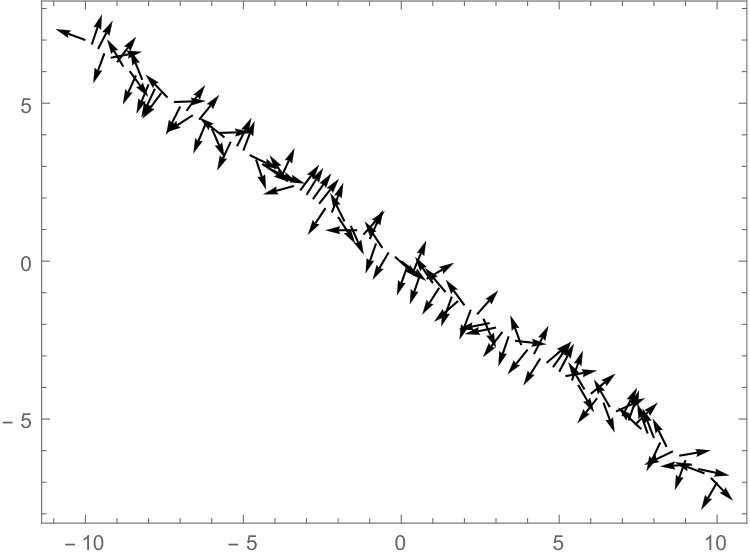 Figure 1
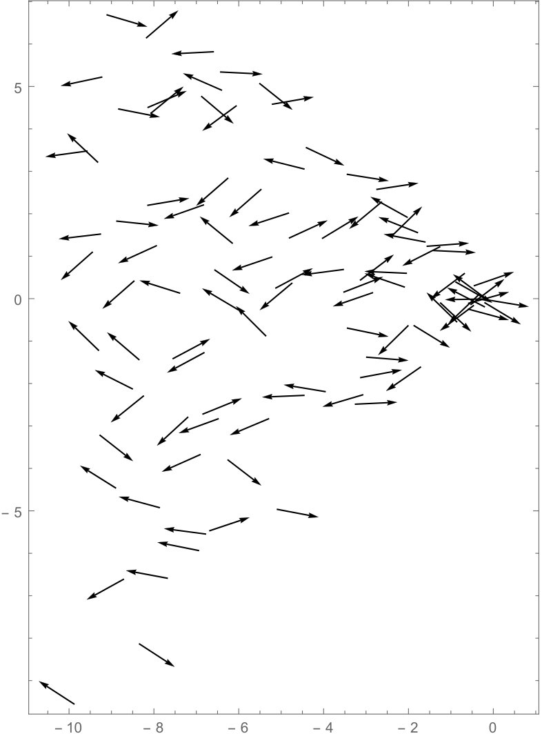 Figure 2
Peer Reviews
No public reviews on file for this paper yet. If you reviewed it on a platform where reviews are public (OpenReview, ICLR, NeurIPS, ICML), you can paste yours below so the community can read it here.
Videos
No videos yet. Explain this paper in a talk, walkthrough, or lecture? Add one.
Wilson lines in the MHV action
P. Kotko and A. M. Stasto
*The Pennsylvania State University, Physics Department
104 Davey Lab, University Park, PA 16802, USA*
Abstract
The MHV action is the Yang-Mills action quantized on the light-front, where the two explicit physical gluonic degrees of freedom have been canonically transformed to a new set of fields. This transformation leads to the action with vertices being off-shell continuations of the MHV amplitudes. We show that the solution to the field transformation expressing one of the new fields in terms of the Yang-Mills field is a certain type of the Wilson line. More precisely, it is a straight infinite gauge link with a slope extending to the light-cone minus and the transverse direction. One of the consequences of that fact is that certain MHV vertices reduced partially on-shell are gauge invariant – a fact discovered before using conventional light-front perturbation theory. We also analyze the diagrammatic content of the field transformations leading to the MHV action. We found that the diagrams for the solution to the transformation (given by the Wilson line) and its inverse differ only by light-front energy denominators. Further, we investigate the coordinate space version of the inverse solution to the one given by the Wilson line. We find an explicit expression given by a power series in fields. We also give a geometric interpretation to it by means of a specially defined vector field. Finally, we discuss the fact that the Wilson line solution to the transformation is directly related to the all-like helicity gluon wave function, while the inverse functional is a generating functional for solutions of self-dual Yang-Mills equations.
Contents
1 Introduction
Through the recent decades there has been great progress in the calculation of the scattering amplitudes in QCD. This is of course indispensable for practical applications, see e.g. [1], and especially in context of the plethora of QCD and electroweak measurements performed at Large Hadron Collider, such as multi-jet production or processes including a production of and bosons. However, amplitudes are also interesting from the theoretical point of view. It turns out that they encode variety of hidden aspects of the theory, even at the tree level. For example, all gluonic amplitudes with two helicity projections different than all other, so-called maximally helicity violating (MHV) amplitudes, appear to have an extremely simple one-term form when expressed in terms of spinor products [2, 3] (see [4] for a review of the spinor helicity methods). Since in the ordinary approach based on the Feynman diagrams this simplicity is not evident (the number of diagrams grows significantly with the increase of the number of legs), the intuition suggests that there has to be a hidden structure or symmetry. Indeed, in the last two decades the understanding of this result in terms of abstract geometry has enormously developed: from the formulation of amplitudes in the twistor space [5] to new mathematical structures like the amplituhedron [6]. Somewhat in parallel, more ‘standard’ but powerful methods based on a generic analytic structure of the Feynman diagrams have also been developed (see e.g. [7] for a review of tree-level and loop-level techniques). One of those is the Britto-Cachazo-Feng-Witten (BCFW) recursion relation [8, 9]. In this recursion, which utilizes analytical properties of the scattering amplitudes, one uses lower on-shell amplitudes with deformed complex momenta to compute the on-shell amplitudes with higher number of legs. Another, somewhat related method but truly motivated by the geometry is the one proposed by Cachazo, Svrcek and Witten (CSW) [10]. Since this is the method that provides the motivation to the present work, let us briefly remind its main elements.
The building blocks of the CSW method are so-called MHV vertices, i.e. MHV amplitudes which are continued off-shell. It turns out that any amplitude can be constructed by combining such vertices using scalar propagators. This twistor-space motivated conjecture has been directly proved by means of the BCFW recursion [9, 11]. In parallel, another beautiful derivation of the method was found; in [12] a canonical transformation of fields was proposed that transforms the light-front quantized Yang-Mills action into a new action which explicitly contains the off-shell MHV vertices. In what follows, we shall refer to that new action as the ‘MHV action’. One of the early issues of that formalism was that all-like helicity amplitudes, which are zero at the tree level but non-zero in general, were not accessible from the action. This issue was later solved in [13, 14, 15, 16]. Further developments in this direction included an explicit construction of the twistor action which leads to the generation of the MHV diagrams [17].
In the present work we reconsider the field transformation used in [12] and show that its solution can be expressed by a particular form of the Wilson line (for a review of Wilson lines in quantum field theory see [18]). This seems to be overlooked in the literature, although the momentum space solution given by a power expansion in the fields is known. This might be due to the fact that the most common usage of the Wilson lines utilizes the light-like (or transverse at the light-cone infinity) straight paths. Here, however, the straight path is defined in the complexified Minkowski space and extends to the light-cone minus and transverse directions. Also, the slope of this Wilson line is integrated over. Since the field transformation is reversible it makes sense to ask about the inverse solution. It is also known in momentum space [13], but since the Wilson line is defined in the position space it is interesting to construct also its position space inverse. The inverse solution is interesting also because it is a generating functional for solutions of the self-dual Yang-Mills equations [19, 20, 21].
An immediate consequence of the fact that the MHV action contains infinite Wilson lines is that one can construct gauge invariant off-shell currents which have the MHV form. Interestingly, such objects were found independently in [22] using the ordinary light-front perturbation theory [23, 24]. Later it was shown, without referring to the CSW method or MHV action, that such gauge invariant MHV currents originate in a matrix element of the Wilson line [25, 26]. It turns out that it is the same Wilson line as the one derived here as a solution to canonical field transformation. We shall discuss these and related topics in detail in this work. Also, using the light-front perturbation theory we shall elucidate the diagrammatic content of the Wilson line solution as well as the inverse transformation.
The structure of the paper is as follows. In Section 2 we set up the notations and conventions used throughout this work. In section 3 we recall the field transformation used to derive the MHV Lagrangian. This section contains mostly known results and is thus introductory. The following sections explore the concepts described above. The next Section 4 contains one of the main results of the work, i.e. the proof of the Wilson line solution. In Section 5 we discuss the construction of the gauge invariant off-shell currents which satisfy the Ward identities, using the Wilson line defined previously. In Section 6 we discuss the diagrammatic content of both the transformation and its inverse. In Section 7 we discuss the inverse transformation in the coordinate space. The geometric interpretation of both transformations in terms of a specially defined vector field in two dimensional space is discussed in Section 8. Finally, in Section 9 we summarize the results and present our conclusions.
2 Notation
We start by introducing the notation and conventions used throughout the paper.
The light cone basis is defined by the two lightlike four-vectors
[TABLE]
and two space like complex four-vectors spanning the transverse plane
[TABLE]
The contravariant coordinates of a four-vector in that basis are denoted as follows
[TABLE]
The covariant components are
[TABLE]
The explicit expansion of a four-vector reads
[TABLE]
The scalar product can be thus written as111Our notation corresponds to the one used in [12] as follows: , , while the plus and minus components stay the same. We found the notation with and as subscripts somewhat cumbersome, especially when raising and lowering the indices.
[TABLE]
The gauge field in the fundamental representation is denoted as
[TABLE]
where are color generators satisfying
[TABLE]
and
[TABLE]
We shall often use the rescaled coupling constant
[TABLE]
Since we shall work within a theory quantized on equal light-cone time surface, defined by , it is convenient to introduce a three vector
[TABLE]
and the corresponding measure
[TABLE]
We reserve (with possible subscripts) to denote three-vectors in position space. Similarly, we introduce momentum space three-vectors (with possible subscripts):
[TABLE]
and the corresponding measure
[TABLE]
Above, we have included the factor in the measure in order to avoid a proliferation of these factors when making the Fourier transforms.
We shall use the following notation and definition of the Fourier transform of fields:
[TABLE]
for fixed . We shall almost always suppress the argument and write simply
[TABLE]
Let us now introduce the essential part of the notation which is equivalent to the spinor algebra. For given four momenta we define the following variables [27]:
[TABLE]
Note, that these symbols are equally well defined for three-vectors . We shall thus not distinguish those situations. The real version of these variables have a very natural interpretation within the light-front perturbation theory. Since component on the light-front can be interpreted as a ‘mass’, the variable can be therefore thought of as the ‘velocity’ in the 2-dimensional space. In addition, it will appear useful to consider the following non anti-symmetric modification of those symbols [25]:
[TABLE]
and similar for . In particular, these variables can be expressed as follows
[TABLE]
where are polarization vectors defined as
[TABLE]
In our applications we shall typically deal with a set of momenta (or ). For that case we will write, for example,
[TABLE]
where
[TABLE]
The symbols satisfy several useful identities which we collect in Appendix A.
As mentioned, the above symbols are directly related to the spinor products:
[TABLE]
where
[TABLE]
Above and are Weyl spinors of positive and negative chirality. The reason for using the symbols instead of spinor products will become clear later.
3 The MHV action
As mentioned in the Introduction, the CSW method [10] was motivated by the twistor theory and later proved by means of the more standard methods based on analytic structure of amplitudes [9, 11]. It was however desirable to construct an explicit action for the MHV vertices. This task was accomplished in [12] by means of certain field transformation performed on the light-front Yang-Mills action. Since the properties of the transformation and the resulting MHV action are central to the present work, we shall now review the main concepts. In order to keep everything consistent (and for educational purposes) we have rederived the MHV action from the scratch, using the notation described in the previous section. For interested readers less familiar with the subject we present more detailed elements of our derivation in Appendix C.
The Yang-Mills action is defined as
[TABLE]
Here, with . The action can be rewritten in terms of the physical degrees of freedom involving two transverse gluon polarizations alone [28]. It is done as follows (see also [12] for this operation in the present context of the MHV vertices). First we rewrite the Yang-Mills action using the light cone coordinates (3) and transverse coordinates (4) (the fact that we use the complexified transverse plane is not essential for this step; one could use just Cartesian components as well). Next, we choose the light-cone gauge . The Yang-Mills action becomes quadratic in , which allows to integrate this field out of the path integral. The resulting action can be written as
[TABLE]
where
[TABLE]
Above we have used the following differential operators acting on functions of :
[TABLE]
The inverse operator is realized through the indefinite integral (see [28] for a particular implementation dealing with the integration constant ambiguity).
The CSW action is now constructed from (28) using a canonical transformation of fields , so that the Jacobian is field independent and such that [12]
[TABLE]
This eliminates the vertex which has only one negative helicity and thus does not belong to the CSW action. The relevant canonical transformation of the field has the form
[TABLE]
The requirement (34) gives the following transformation for the field
[TABLE]
where the differential operator is defined as
[TABLE]
The relation (36) holds on the constant hyper-surface.
In order to obtain the new action , in principle, one has to solve the equations (35),(36) for and and insert the solutions to the action (28). However, in the original work [12] the new action was constructed using only analytic properties of the transformations and equivalence theorem for the S-matrix. The explicit solution for and fields was found in [13] in momentum space. Within our conventions the solution for reads (see also Section 6.2)
[TABLE]
with
[TABLE]
Above, the curly brackets indicate that the function is symmetric with respect to the pairs enclosed by the brackets and that the result for was obtained utilizing the fact that the enclosed arguments are integrated/summed with the fields. Sometimes we shall refer to such equality as the equality in the ‘weak sense’. For example, the following expression
[TABLE]
where is the permutation group, and
[TABLE]
is different than (39). However
[TABLE]
thus they are equal in the ‘weak sense’.
The solution for (see Appendix C) is
[TABLE]
with
[TABLE]
The above transformations, when applied to give the MHV action:
[TABLE]
where the part of the Lagrangian for interaction of fields is
[TABLE]
This interaction term corresponds to the MHV vertex with two gluons with minus helicities, corresponding to the fields, and the rest of the particles, corresponding to fields, having plus helicites. It is convenient to decompose the MHV vertex into color-ordered objects, similar to what we did in (40) (this technique is often used for multi leg QCD amplitudes, see [4] for a review)
[TABLE]
Then one finds
[TABLE]
When written in terms of spinors using (25) we see that they look like the Mangano-Parke amplitudes, except that they are fully off-shell objects. This is one of the reasons we prefer to use the symbols instead of spinors. The latter are normally defined for on-shell momenta and need a prescription to be continued off-shell, in general situation.
In the original formulation [10] the spinors in the MHV vertices were defined using an analytic continuation to the off-shell momenta by means of an additional auxiliary on-shell momentum. In the context of the action (45) the off-shell continuation means that we can use any for fixed . components of the momenta. They are the components that determine the vertex. In fact, the spinor products can be constructed without a reference to , see Eq. (25). Obviously, the off-shell continued spinors will coincide with the on-shell spinors with the same , fixed by the on-shell condition . One can also look at this from another point of view. In light front quantized theory the internal lines in the Feynman diagrams are on-shell (see e.g. [29]) at the cost of the energy denominators involving components. Thus in that case the spinors can be defined for any internal line. This fact was used for instance in [27] to express the vertexes in terms of spinors.
In the next section we shall take a closer look at the transformation (36). In particular we shall consider a solution expressing the field in terms of fields and see that it gives a new interpretation to the MHV vertices.
4 Wilson line solution to the field transformation
In the previous section we have recalled the procedure to obtain the MHV action. The essential step is to solve the transformation (36) and find the functional , so that the new action can be expressed in terms of fields only, with the infinite set of MHV vertices. Now, it is extremely interesting to study the true physical meaning of the new fields, in particular the field. As we will show in the following section it turns out that it is a certain type of straight infinite Wilson line.
Let us introduce a four-vector
[TABLE]
where is a real parameter and the vectors and were defined in Section 2. In the coordinates it reads
[TABLE]
Let us then postulate the solution to the equation (36) in the following form
[TABLE]
where denotes the path ordering of fields with increase of the parameter . This path exponential is in fact the Wilson line (for a modern review of the Wilson lines in quantum field theory see [18]). Indeed, taking the path to be
[TABLE]
we have
[TABLE]
where we have used the gauge condition . The idea of using non-lightlike Wilson lines with a slope defined to be a vector reminiscent of the polarization vector (compare (49) and (22); see also explanation below) is motivated by a procedure presented in [30], where such objects were used to construct off-shell amplitudes which satisfy Ward identities.
Notice the integral over in (51) which means that the summation over all slopes has to be taken into account.
We now prove that (51) is the solution to (36). It is convenient to perform the proof in the momentum space. Let us thus write the expansion of this solution in momentum space
[TABLE]
Let us calculate the -th coefficient of the expansion . To this end, consider the -th term in the expansion of the Wilson line
[TABLE]
For the ordered integrals we get
[TABLE]
Above we have used the notation . The result is a generalized function as is evident from the prescription. The existence of such prescription can be proved by considering a limit of a non-straight almost infinite path [30].
Coming back to (55) using the form of and definitions (20) we arrive at
[TABLE]
In what follows we shall omit the prescription.
Comparing (54) with (57) we get
[TABLE]
where we have used the property (5) from Appendix A to get the last equality.
Now we will prove that it satisfies the equation (36). In Section 6.1 we shall show that assuming (36), the expansion coefficients satisfy the following recursion (see also [12] for a similar recursion in position space)
[TABLE]
In the equation above we introduced the quantity
[TABLE]
It is a so-called energy denominator known from the perturbation theory on the light front [31] (see Section 6.1 for a justification of that statement). Equation (59) should be understood in the ‘weak’ sense as explained in the previous section, i.e. upon integrating with the fields over momenta (and summing over color indices). To complete the proof we first note, that for we have (from (55))
[TABLE]
For we have (from (58))
[TABLE]
Let us compare this with what one gets from recursion (59). We have
[TABLE]
Remembering that it is to be integrated with we can change variables for the first term and using arrive at
[TABLE]
which equals . Now we proceed to an arbitrary . We consider the r.h.s of (59) and insert (58) and obtain
[TABLE]
We turn each term in the bracket into pure traces. For example, for the first term we have
[TABLE]
and so on. Next, we use the fact that it has to be integrated with the gauge fields. Thus, we can change variables for each of the second term arriving from the tensor expansion: , and so on. Using
[TABLE]
we get
[TABLE]
Using now the relation (131) we arrive at
[TABLE]
which is exactly obtained in Eq. (58). Thus, indeed Wilson line (51) is a solution to the transformation (36).
It is convenient to introduce the Feynman rules for the Wilson line. Following the standard treatment [32] the propagators are given by the denominators in (56) while the vertex is just :
[TABLE]
Using these elements, the -th term in the expansion of the field can be represented by the following diagram:
[TABLE]
Above, the trace over color matrices is understood. The field thus has the following simple diagrammatic expansion:
[TABLE]
In the next section we shall study an immediate consequence of this result.
5 Gauge invariant off-shell currents
As demonstrated in the previous section, the interaction terms (46) in the MHV Lagrangian contain the infinite Wilson lines encoded in the fields. This has interesting consequences which we shall explore below in the current section.
Let us consider the MHV vertex, where all fields except one with negative helicity (corresponding here to the field ) become on-shell. Thus, more formally, we consider a current for a transition of an off-shell particle given by the field (a ‘gluon’ in the action ) to a set of on-shell ‘gluons’ given by the fields
[TABLE]
where the momentum space Green’s function reads
[TABLE]
It is understood that, in the above expression only connected contributions are taken into account. Elementary tree level calculation leads to the anticipated result
[TABLE]
with being the MHV vertex (47). Above, the momenta are on-shell.
Now, let us consider the same current in terms of , fields. Since we work at tree level, we may replace all on-shell , fields by , due to the -matrix equivalence theorem (stating that a reversible field transformation does not change the -matrix up to a wave function renormalization, which, however, does not matter at the tree level). Thus we have
[TABLE]
This can be interpreted as a matrix element of the Wilson line operator
[TABLE]
where the kets represent on-shell gluons with definite helicity. Since the Wilson line extends from to it is gauge invariant with respect to the small gauge transformations. This fact together with on-shellness of the remaining gluons means that the whole object is gauge invariant. It was explicitly demonstrated using the Slavnov-Taylor identities for a similar link operator in [30]. In terms of color ordered Feynman diagrams, (77) can be expressed as
[TABLE]
where the blobs represent the ordinary gluonic off-shell currents given by the sum of standard Feynman diagrams. Let us denote these currents as
[TABLE]
where denote the helicity corresponding to the leg . Note, that the currents considered here have no free vector index, but are projected on a polarization vector corresponding to .
The off-shell currents with the MHV helicity configuration defined as (77) were considered before in the context of the recurrence relations for amplitudes within the light-front perturbation theory [25, 26] (for a review see [29]). Let us briefly recall the main results, as they are tightly connected to the present work. Suppose one wants to solve the light-front version of the Berends-Giele relation for the MHV configuration, that is, one wants to find an off-shell current for any . The task was accomplished in [22] and the result reads (we work with color amplitudes for brevity)222The results in [22, 25, 26] consider ‘mostly-plus’ MHV configuration while the present work would correspond to ‘mostly-minus’ MHV amplitudes in these works. Here we have adapted the cited results to the present helicity convention.
[TABLE]
where the structure on the r.h.s. appeared somewhat naturally, with both quantities and derived by summing certain light-front diagrams. First, is a current for transition of a minus helicity off-shell gluon to all plus on-shell gluons and reads
[TABLE]
Note that this is identical to – a fact to which we come back later in Section 6.2. Second, the auxiliary quantity turned out to have the MHV form, despite being off-shell. In fact
[TABLE]
which is exactly (75) (up to the momentum conservation delta function)
[TABLE]
Later, in [25, 26] it was shown that this result has indeed its origin in a matrix element of Wilson line, identical to (77), which here we have derived from the MHV Lagrangian. Actually, in [25, 26] the Wilson line slope was fixed and taken to be (with the present notation) . Here the slope is , but as seen in the detailed computation from Section 4 the integration over in (51) sets when the Fourier transform is taken.
To conclude, when considering recurrence relations within the light-front perturbation theory, the partially reduced CSW vertex appears naturally. Moreover, it is a matrix element of the straight infinite Wilson line, thus it is gauge invariant which makes the resulting expressions simple, cf. (80). In the present paper, we have proved that property directly from the MHV Lagrangian showing that in fact, the new field is expressed by the Wilson line.
Finally, let us notice that another class of gauge invariant currents (or amplitudes) can be constructed by retaining both fields off-shell. The resulting off-shell amplitude will have simple MHV form and will be again gauge invariant (see the demonstration with two Wilson lines in Ref. [30]). This property for similar amplitudes with two off-shell legs was also observed in [33] in the context of the high energy scattering, where the off-shell gluons have only longitudinal polarizations.
6 Inverse transformation and energy denominators in the light-front theory
In this section we take a closer look at the solutions to the field transformation (36), and , using the Feynman diagrams in momentum space. The main motivation to do this comes from calculations of the wave-functions and fragmentation functions [27] within the light-front perturbation theory [23, 24]. Let us recall that in the light-front approach all lines are treated on-shell (in the sense of having ) with the transverse polarizations and one has to sum over various light-cone time orderings. Instead of propagators, the intermediate states are assigned energy denominators, similar to the non-relativistic quantum mechanics. The energy denominator is the difference between the sum of light-cone energies of the intermediate states, and the light-cone energy of the reference state (being the final or initial state).
We want to draw attention to two interesting results derived in [27] using the light-front perturbation theory: (i) the calculation of the -gluon component of the gluon wave function with the helicity configuration ; (ii) the calculation of the fragmentation function of a gluon with the helicity configuration . Those two cases differ by the interpretation of the initial and final states. For (i) the initial gluon is on-shell and it splits to the -gluon intermediate state (being thus off-shell). For (ii) an intermediate gluon state splits to bunch of final state gluons which are on-shell. Thus the cases (i) and (ii) differ only by the usage of energy denominators, more precisely, they differ only by a reference state which defines the energy denominators: final or initial state. Yet, it turns out that the result for both cases are very different. Now, the interesting point is that the wave function (i) corresponds exactly to the expansion coefficients of the momentum space solution , while the fragmentation function (ii) corresponds exactly to the expansion coefficients of the solution . Thus the coefficients of the inverse transformation can be obtained by taking the same diagrams, but slightly different energy denominators.
Below, we derive the coefficients and using the light-front diagrams and confirm the above statements.
6.1 The diagrammatic content of
In Section 4 we have obtained the solution using the Wilson line. Here we derive the solution by working directly in momentum space and introducing light-front diagrams. This is somewhat similar to what was done in [12], but there the iterative solution was given in position space and no reference to light-front diagrams was given.
Similar to Section 4 we express the field as a power expansion in fields. In momentum space we have
[TABLE]
where the symbols are symmetric in pairs of indices . We use different symbols for the expansion coefficients than in Section 4 not to pre-assume they are identical.
It can be demonstrated (see Appendix B) that the coefficients satisfy the following recursion relation
[TABLE]
where
[TABLE]
is the vertex appearing in the Lagrangian (see Eq. (189)). The light-cone energy is
[TABLE]
The symmetry factor reads
[TABLE]
The equation (85) can be graphically represented as follows
[TABLE]
It is convenient to introduce the color decomposition for
[TABLE]
where is the permutation group. Solving the color-ordered analog of the recursion (85) (see Appendix B) we obtain
[TABLE]
It is easy to see that (90) with (91) is exactly (58) in the ‘weak sense’. On the other hand, calculating a few first terms in the recursion (85) (see Appendix B) we see that the expansion of field has the following diagrammatic content:
[TABLE]
Above the vertical dashed lines represent the energy denominators where
[TABLE]
Above is the energy of the initial state and is the sum of energies of the lines that the cut crosses through (the intermediate states). In addition, as usual in the light-front perturbation theory, a factor is assigned to each intermediate state.
It is interesting that the sum of the light-front diagrams containing the triple gluon splitting given by (86) and energy denominators collapses into factors like (91). As mentioned, this was for the first time shown in [27] without any reference to the MHV action. In Section 4 we have shown, that they in fact are the expansion coefficients of the Wilson line (51) in momentum space. Thus, the gluon wave function with gluon components with all-like helicities is given by the Wilson line (51).
6.2 The diagrammatic content of
Consider now the inverse transformation, that is an expansion of field in terms of in momentum space:
[TABLE]
The expansion coefficient functions are symmetric in pairs of indices . These functions have been derived in [13]. Here we will concentrate on their diagrammatic content and the relation to coefficients.
Inserting the expansion (94) to (84) and comparing coefficients with the same number of fields we can derive a set of equations. For the two-point function we have
[TABLE]
For the three-point function we get
[TABLE]
and so on. It is convenient to express the above recursion in a diagrammatic form. Showing the planar diagrams only we have for :
[TABLE]
For we obtain
[TABLE]
[TABLE]
and so on. This can be expressed entirely in terms of the known functions. Consider, for example, the function. Using the fact that and utilizing the result for we have
[TABLE]
The first (second) diagram differs from the third (fourth) only by the one of the energy denominators. Noticing that
[TABLE]
where , etc., we can write (99) as
[TABLE]
The double dashed line now denotes the energy denominators defined with respect to the final states:
[TABLE]
where the first sum runs over the energies of the final states, while the second sum runs over the energies of the intermediate states. In our example, some of the relations to the old denominators are
[TABLE]
and so on.
It is easy to see, that can be all calculated from similar diagrams. In fact, one can calculate from the following recursion relation (being in fact the light-front equivalent of the Berends-Giele recursion [3], the so-called cluster decomposition [34])
[TABLE]
The standard Berends-Giele recursion for all-like helicity currents was solved long time ago in their original paper [3]. The above light-front version has been solved in [27] (see also [25, 26] for different methods to solve it, using gauge invariance). The nature of the above diagrams, in particular the nature of the energy denominators, allows to identify with the fragmentation functions considered in [27]. In fact, the resulting expression for color-ordered reads
[TABLE]
and it agrees with the results of [27] (modulo pre-factors due to the normalization conventions). It also agrees with [13].
Thus we have shown that mere change of energy denominators in the diagrams contributing to transforms them into , which are the coefficients of the inverse functional. The coefficients are the expansion coefficients of the Wilson line (51) in momentum space. Thus a natural question arises as to what is the inverse functional in coordinate space, i.e. an inverse of the Wilson line.
7 Inverse transformation in position space
We saw that the solution
[TABLE]
is given by the Wilson line defined in (51). On the other hand, the power expansion coefficients of that solution and of the inverse solution
[TABLE]
have interesting symmetry. As seen in the previous section, they contain the same light-front Feynman diagrams, but the energy denominators for the intermediate states are calculated with respect to different reference light-front energy, i.e. corresponding to either initial or final state.
Because of that observation, it is tempting to investigate how those two solutions differ in the position space. Thus, in this section we construct an inverse functional to the Wilson line (51). Looking at (recall that ) and comparing with gives an idea of how to construct the inverse position space solution. Namely in we see a chain of denominators containing terms. They are easily understandable from the Feynman rules, see (71). Since, the slope of the Wilson line is the consecutive double line propagators contribute
[TABLE]
Now, looking at the expression for (107), we see that one could think of a ‘Wilson line’ which changes the slope after every emission to the polarization vector of the emitted gluon.
Using the above observations as a guidance, we find a suitable functional and prove that it has expansion in terms of in momentum space.
Consider a generic matrix-valued field . Let us define the following functional
[TABLE]
where the vector is defined in Eq. (50). The variables and run over the whole space. We claim that
[TABLE]
In order to prove it, let us consider the -th term in (112) and let us pass to the momentum space:
[TABLE]
Performing elementary calculations similar to those in Section 4 we get
[TABLE]
The final formula reads
[TABLE]
We see, that (114) exactly reproduces .
In the end, let us mention that the functional is actually the generating functional for the position space solutions to the self-dual Yang-Mills equations [19] (see also [35, 36, 37, 20]). Namely
[TABLE]
This gives expressed in terms of delta functions and Heaviside step functions.
8 On the geometry of functionals and
In the previous section we have constructed the functional inverse to (51), given by (112) with (111). The Wilson line solution has a very clear geometrical interpretation. Namely, the gauge fields lie on a line given by the path (52) with a slope , which is ultimately integrated over. In this section we suggest a geometrical interpretation for the inverse solution. To do so we shall construct a 2D space on which we will represent expansion (111) using certain vector field. We shall apply the same construction for both functionals and to represent them both in a unified way.
To this end let us consider a generic field (can be or ). Let us define the following object:
[TABLE]
where the vector is defined in Eq. (50). Notice that for these are the objects that appear in (111). Above the point is fixed once and for all. The parameters . Next, let us note that the three-vectors actually have only two non-zero components, see (50). Therefore
[TABLE]
can be thought of as a real coordinates on a 2D plane.
Therefore, consider an affine space consisting of the points
[TABLE]
For our purposes, it is convenient to parametrize any point in that space by the ‘slope’ and the parameter
[TABLE]
In particular, a point corresponding to the vector has coordinates
[TABLE]
This is illustrated in left of Fig. 1.
The object (117) can be thought of as a vector field attached to the point with a direction given by . The magnitude is given by the integral in (117) and of course can vary from point to point. For simplicity we shall represent as an arrow with some fixed length attached in the point and oriented along , see right of Fig. 1.
Consider now the following object
[TABLE]
which – according to the construction above – may be identified with a set depicted in left of Fig. 2. So far, the objects we considered were defined for an unspecified scalar field . Here we want to work with matrix-valued gauge fields or , thus we need to be careful about the exact order of objects in expressions like the one above. To underline that we now deal with the matrix-valued objects we put the hats:
[TABLE]
Let us now show, that the following integral
[TABLE]
is directly related to the -th coefficient in the expansion of the Wilson line in (51) (when of course). This is most readily performed in the momentum space. We use (117) and perform the Fourier transform
[TABLE]
Note, that
[TABLE]
and we are left with
[TABLE]
which is exactly the same chain of integrals as in (55) up to normalization prefactors which are not essential for the present discussion.
Thus, to conclude, the solution given by the Wilson line can be represented by the infinite sum of the objects like the one in Fig. 2.
Now, let us come back to our original question, which now can be formulated as follows: what is the geometric object in our 2D space the inverse functional (111) corresponds to?
Let us consider the -th term from the (111):
[TABLE]
First, note that the expression does look asymmetric as the first field does not have a derivative and the -dependent part. It can be however easily put into a symmetric form as follows:
[TABLE]
Let us represent it in terms of the vectors . Similar as in (124) we will fix the parameter (in (124) as well as here it will be integrated over in the end). Denoting the corresponding chain of vectors by we have
[TABLE]
The above integrand is represented in right of Fig. 2.
There is one comment in order here. The integrals over positions , are not ordered here (compare Eq. (124)). This is in fact not required to maintain the order, as each vector has different direction and there is no risk of misplacing them.
To summarize, the functionals and , (108), (109), can be characterized by two entirely different supports and ordering of the fields. The functional which contains the Wilson line can be characterized by a vector field supported on an ensemble of lines crossing the origin in the 2D space, see Fig. 3 left. The orientations of the vectors have to be integrated over. The order of vectors is given by the parameter along the line. On the other hand, the inverse functional, , is characterized by a vector field scattered across the plane. The positions and orientations of vectors have to be integrated over. The order is defined by the orientations of the vectors: the preceding vector orientation determines one coordinate of the position of the following vector, see Fig. 3 right.
9 Summary and conclusions
This work was motivated by several interesting results obtained previously within the light-front perturbation theory. First, by the solution to the light-front recursion relations for the amplitudes with MHV helicity configuration [22]. It was observed that, in the off-shell current which is the solution to the recursion, appeared an object which had exactly the MHV form despite the fact that it was off-shell. Thus it resembled the MHV vertex which appeared in the CSW formalism. In [25] it was demonstrated that in fact this object can be calculated from a matrix element of straight infinite Wilson line and thus it is gauge invariant (see Section 5). Therefore it was a natural expectation that the transformation (36) leading to the MHV Lagrangian contained Wilson line as well. In Section 4 we have proven that this is indeed the case. The straight infinite Wilson line solving the transformation is however different than what one can typically find in the literature. Namely, the slope of the line is defined by a polarization-like vector , where the parameter sets the longitudinal component of the vector, see (49). This parameter is integrated over in the Wilson line (actually its derivative). In the momentum space the integration over effectively sets to be equal to the polarization vector for momentum of the Wilson line.
Another direction of study, motivated by the light-front perturbation theory, in particular results of [27], was to investigate the diagrammatic content of the field transformation (36). As demonstrated in Section 6 it turns out that the Wilson line solution and the inverse solution differ only by the definition of the light-front energy denominators, containing otherwise the same gluon cascade. In [27] the same observation distinguishes the gluon wave function (with on-shell initial state) and the gluon fragmentation function (with on-shell final states). In the latter work it was also observed that, under certain kinematic assumption, both objects are dual, in the sense that if one transforms one of them to position space, the resulting expression will equal the second if positions are simply replaced by momenta. This motivated a study of the inverse solution, i.e. , in the position space. Such inverse solution was constructed in Section 7 and it is given by a simple power expansion in fields with shifting arguments along certain directions, see Eq. (111). Unlike the Wilson line, which is supported on an ensemble of infinite straight lines in a 2D space, the inverse solution is scattered over the whole plane (see Section 8).
The inverse solution to the one given by the Wilson line is interesting also on its own. The coefficients of its momentum space expansion in powers of fields can be identified with the off-shell currents for all-like helicity gluons. The latter are the solutions to the self-dual sector of the Yang-Mills equations [19]. In fact, the transformation leading to the MHV action transforms the self-dual part into the kinetic part of the new action (see also [21]). On the other hand the self-dual Yang-Mills equations are closely connected to integrable systems [38]. Thus, it might be interesting to investigate whether the position space forms of the solution – the one that generates the self-dual solutions and its inverse given by the Wilson line – might be useful in that matter.
There are several further potential directions of study which we briefly outline below.
One is a question related to the high energy limit of QCD. Namely, in [39] a gauge-invariant effective action for high-energy QCD was proposed. The crucial element of this action are new fields, which are in fact Wilson lines when the equations of motion are utilized. Those Wilson lines have different slope though, then in the present case (being simply the light-cone direction). However, the structure of the MHV vertices with Wilson lines (51) resembles the structure of vertices in that theory. Thus, it would be interesting to investigate if the high-energy limit of the MHV action could be taken and how it would be related to the high-energy effective action proposed in [39].
Another potential direction of study concerns loop corrections. It is known that the MHV action (45) is not complete at loop level. As recalled in the Introduction, two solutions have been proposed. One based on the dimensional regularization and evasion of the S-matrix equivalence theorem [14], and another using world-sheet regularization [15] which leads to additional term in the light-cone action (28) and thus additional terms in the MHV action. The question is whether the information that the solution to transformation is given by the Wilson line might be helpful, in the sense, that the renormalization of Wilson lines is a known issue from many aspects.
Acknowledgements
We are grateful to Lance Dixon and Mirko Serino for turning our attention to the CSW construction. We also acknowledge discussions with Radu Roiban and Leszek Motyka.
The work was supported by the Department of Energy Grants No. DE-SC-0002145, DE-FG02-93ER40771 as well as the National Science Center, Poland, Grant No. 2015/17/B/ST2/01838. The diagrams were drawn using the Jaxodraw [40].
Appendix A Useful identities
For reader’s convenience we collect some of the properties of the symbols introduced in (20).
, but 2. 2.
3. 3.
4. 4.
5. 5.
for
For more relations and their proofs see [25]. Plenty of useful identities for symbols are contained in [27, 22], which of course can be translated to symbols.
In particular, in the present work we shall need the following identity (adapted from [27]):
[TABLE]
where the energy denominator (see Eq. (93)) has been expressed in terms of symbols, see Eq. (60).
Appendix B Recursion relation for field
In this appendix we derive and solve the recursion (85). We start the calculation in the position space, and later we shall convert to the momentum space. The field has the following power expansion in fields:
[TABLE]
The symbols are symmetric in pairs of indices .
We shall start with the l.h.s. of (36). The functional derivative reads
[TABLE]
Using the expansion (132) and (133) in the l.h.s. of (36) we have
[TABLE]
From this we derive the -th term in the expansion:
[TABLE]
Comparing this with the r.h.s of (36) with (132) we have for the same power of field
[TABLE]
We shall now make Fourier transform to the momentum space. The new coefficients are defined as the Fourier transform of functions in the following way
[TABLE]
The transform of gluon fields is given in (17). The expansion of in terms of fields in the momentum space is given by (84). We arrive at
[TABLE]
where is defined in (87). Let symmterize the first term as follows:
[TABLE]
where we have used the vertex
[TABLE]
with . In what follows we shall use shorthand notation
[TABLE]
Next, we symmetrize the second term of the l.h.s of (138):
[TABLE]
Thus, the equation for the reads
[TABLE]
or simply
[TABLE]
Above, we understand the equality in a ‘weak’ sense, that is we keep in mind that we can ultimately integrate it with the fields.
Let us note, that we can write the r.h.s. as a sum of terms with the vertex insertion for all combinations of the momenta. This is simply done by writing it as a sum with an appropriate symmetry factor and performing a suitable exchange of the integration momenta and color indices. This procedure is necessary if we want to apply the color decomposition, and is illustrated graphically in (89). We observe that the planar contributions give terms on the r.h.s of (144). Including in addition the non-planar contributions we get finally the following symmetry factors
[TABLE]
The final result for the recursion reads
[TABLE]
The first two coefficients of the expansion read
[TABLE]
[TABLE]
where we used the shorthand notation for the sum of the momenta (24) and (93). The notation means that has to be treated as an intermediate state with the energy . The diagrammatic expansion (92) follows from the above results.
The recursion relation for the color ordered coefficients can be derived in the following way. One can use (146) and decompose , into color ordered amplitudes. Consider the order . We pick up the term from and observe that the multiplying vertex contains which fills the trace thanks to the identity . Moreover
[TABLE]
where
[TABLE]
is the color-ordered vertex. Thus, for the color-ordered amplitudes the recursion (146) has the form
[TABLE]
We can easily find a few first terms from this recursion
[TABLE]
where we used
[TABLE]
Next term reads
[TABLE]
In a similar way we can find that
[TABLE]
We postulate that the solution has the form
[TABLE]
One can prove the above result in a way similar to the Wilson line solution, except that here we are dealing with color-ordered objects, which simplifies the entire procedure. We insert (156) into the color-ordered version of (146). First, note that according to the ansatz (156) we have (we skip momentum conservation delta functions in what follows)
[TABLE]
Using this, we have for the r.h.s. of (146)
[TABLE]
Noticing that
[TABLE]
and utilizing (131) the color ordered solution becomes
[TABLE]
which completes the proof.
Finally we note that, using (90), integrating it with the fields and changing the pair of color/momentum variables we can write the field expansion coefficient simply as
[TABLE]
which is identical to .
Appendix C Rederivation of the MHV action
In this appendix we collect together the elements necessary for the derivation of the MHV action [12]. We have organized it in several parts. The first one deals with the light-front quantization of the Yang-Mills action, while the remaining parts are devoted to the canonical field transformation, its solution, and the derivation of the sample MHV vertex.
C.1 The Yang-Mills action on the light-front
We start with the Yang-Mills (Y-M) action
[TABLE]
where the field strength tensor is
[TABLE]
(See Section 2 for our conventions and notation.) Expanding the action we get explicitly
[TABLE]
Using the LC variables, we rewrite each of the terms in (164) and impose the light-cone gauge condition:
[TABLE]
We divide the Lagrangian into the kinetic part, triple-coupling part, and four-gluon part
[TABLE]
We start with the kinetic term. After some algebra and integration by parts (assuming all fields components vanish at infinity in any direction) we get
[TABLE]
Noticing that
[TABLE]
we can write the kinetic term as
[TABLE]
For the triple-gluon coupling we get:
[TABLE]
Finally, the four-gluon coupling term reads
[TABLE]
The Lagrangian (166) is quadratic in so following [28, 12] one can integrate this field out. Let us note, that actually the Lagrangian is quadratic in all fields; however, the quadratic terms for the transverse fields contain field-dependent operators, which in turn would introduce the field dependent determinant (after integrating over paths).
Let us collect the part of the action dependent on the field:
[TABLE]
This can be written as
[TABLE]
where
[TABLE]
Let us define a new field
[TABLE]
The operator is can be realized by an antiderivative. The action in terms of new field reads (after some algebra and integrating by parts)
[TABLE]
The path integral over fields is Gaussian and thus can be readily performed:
[TABLE]
This is a field independent infinite constant which can be discarded.
Thus, we end up with the following Yang-Mills Lagrangian, expressed in terms of two transverse field components:
[TABLE]
The above action mixes various terms between the ones in the original formulation and the terms appearing due to the integration over field. In order to find the Feynman rules one needs to rewrite slightly this action. Let us start with the kinetic term. Collecting all bilinear terms and integrating by parts we get
[TABLE]
The trilinear contribution reads
[TABLE]
After some tedious algebra, integration by parts and usage of the following relation (applicable for functions vanishing at infinity)
[TABLE]
it simplifies to
[TABLE]
where we defined the operators
[TABLE]
In terms of algebra-valued fields this reads
[TABLE]
In order to find the vertex one needs to perform the Fourier transform to the momentum space. For the field coupling, which corresponds to the ‘’ configuration, we get (after a proper change of indices and integration variables)
[TABLE]
This can also be written as
[TABLE]
with
[TABLE]
The mirror symmetric contribution reads
[TABLE]
with
[TABLE]
Let us proceed to the term with the four-gluon coupling. The original quartic coupling present in the action (164) reads
[TABLE]
The term originating from the integration over contributes:
[TABLE]
Thus total quartic coupling is
[TABLE]
This form accommodates the so-called Coulomb instantaneous interactions. After a little algebra we get in the momentum space
[TABLE]
where
[TABLE]
One can also show that in position space in terms of matrix-valued fields the quartic coupling can be written in a compact way as
[TABLE]
C.2 The field transformation
The idea is to introduce new fields in place of the fields such that the new kinetic term accomodates the ‘’ vertex which does not appear in CSW action [12]
[TABLE]
Writing this explicitly we have
[TABLE]
The transformation is assumed to be canonical, which leads to a simple choice
[TABLE]
and
[TABLE]
We will use it in (197) to eliminate the field. Then, after some algebra, the relation (197) becomes
[TABLE]
Integrating by parts and using
[TABLE]
we get
[TABLE]
Using (199) we get
[TABLE]
The field is an arbitrary function here, thus we can write
[TABLE]
Let us next notice, that if
[TABLE]
i.e. depends on only through it follows that
[TABLE]
as can be easily seen. Therefore we get
[TABLE]
which can be compactly written as
[TABLE]
C.3 Solutions to field transformations
In order to construct the MHV action one needs to replace , fields in the remaining interaction terms to express them through , . Thus we need solutions to (208) and (199), , . The solution has been discussed in Section 3 so we do not repeat it here.
We will find . The relation between and fields in given by (199). We assume the following expansion
[TABLE]
The goal is to find the coefficient functions . We shall find a few first terms and generalize the result. The induction proof for any can be found in [13].
First, the r.h.s. of (199) reads
[TABLE]
where we have used the symmetry of symbols. Using the expansion for fields we have
[TABLE]
Therefore
[TABLE]
[TABLE]
and so on. Passing to the momentum space we have for
[TABLE]
Therefore
[TABLE]
where the bar sign in symbols denotes the inverted momentum. From the definition we have the properties:
[TABLE]
[TABLE]
Thus
[TABLE]
Also we have
[TABLE]
Therefore we can find the relation between the two coefficients
[TABLE]
For we have
[TABLE]
which leads to
[TABLE]
Let us rewrite the appearing above as (taking into account the convolution in and omitting the delta function)
[TABLE]
where we used . The appearing in (222) reads
[TABLE]
Using these to calculate we get
[TABLE]
where the sum in the last line is over permutations of pairs indicated. The first line in the bracket can be written as
[TABLE]
Let us note that this term can be rewritten in as follows (in the ‘weak sense’):
[TABLE]
Now we have
[TABLE]
Calculating the terms in square brackets, after some algebra using (216),(217) and relations from (A) we get for the first term:
[TABLE]
Similar calculation follows for the rest of the terms. We obtain
[TABLE]
This can be again expressed using . After some algebra we get
[TABLE]
So, finally
[TABLE]
Note we have skipped the symmetrization brackets for . This means that it is given by the sum of color ordered amplitudes (40), not by the expression (39).
This can be generalized to
[TABLE]
C.4 The MHV vertices
In this appendix we shall rederive the two lowest vertices in the MHV action. In [13] five-point vertex was also calculated and the general proof can be found in the original paper [12].
The goal is to find
[TABLE]
where are the interaction terms with the MHV vertices.
The first term is simply
[TABLE]
where
[TABLE]
We want to write the vertex using color-ordered amplitudes
[TABLE]
We find
[TABLE]
To get the second term we have to expand the fields. Retaining only the four-field component we get from the three-point part:
[TABLE]
Changing the integration variables to correspond to the ‘external’ momenta and helicity and symmetrizing to involve all the color orderings
[TABLE]
The four-gluon part reads (at lowest order in fields)
[TABLE]
where
[TABLE]
This should be symmetrized as follows:
[TABLE]
We are looking for the following form of the new effective MHV coupling:
[TABLE]
where we will use the color decomposition to present the new effective vertex in a simplest form:
[TABLE]
Let us calculate the contribution. Converting (238) into the color traces we find that only the first, fourth and fifth term contributes here. The first term reads
[TABLE]
Since
[TABLE]
we see that the contribution to from that term is
[TABLE]
Similar, we find from the remaining terms
[TABLE]
The quartic contribution to order comes from the first term in (241). Decomposing the chain into traces we get
[TABLE]
Now, the total MHV vertex reads
[TABLE]
After some algebra we obtain
[TABLE]
We have also calculated some other color orderings and have similar structure.
This can be further generalized to any number of fields:
[TABLE]
The reference list from the paper itself. Each links out to its DOI / PubMed record.
- 1[1] A. Freitas, Numerical multi-loop integrals and applications , Prog. Part. Nucl. Phys. 90 (2016) 201–240 . · doi ↗
- 2[2] S. J. Parke and T. R. Taylor, Amplitude for n-Gluon Scattering , Phys. Rev. Lett. 56 (jun, 1986) 2459–2460 . · doi ↗
- 3[3] F. Berends and W. Giele, Recursive calculations for processes with n gluons , Nucl. Phys. B 306 (sep, 1988) 759–808 . · doi ↗
- 4[4] M. L. Mangano and S. J. Parke, Multi-parton amplitudes in gauge theories , Phys. Rep. 200 (feb, 1991) 301–367 , [ hep-th/0509223 ]. · doi ↗
- 5[5] E. Witten, Perturbative gauge theory as a string theory in twistor space , Commun. Math. Phys. 252 (2004) 189–258 , [ 0312171 ]. · doi ↗
- 6[6] N. Arkani-Hamed and J. Trnka, The Amplituhedron , J. High Energy Phys. 2014 (oct, 2014) 30 . · doi ↗
- 7[7] J. M. Henn and J. Plefka, Scattering amplitudes in gauge theories .
- 8[8] R. Britto, F. Cachazo and B. Feng, New recursion relations for tree amplitudes of gluons , Nucl. Phys. B 715 (may, 2005) 499–522 , [ hep-th/0412308 ]. · doi ↗