Pairing from dynamically screened Coulomb repulsion in bismuth
Jonathan Ruhman, Patrick A. Lee

TL;DR
This paper proposes that superconductivity in bismuth arises from dynamically screened Coulomb interactions, enhanced by plasma modes and electronic structure, rather than conventional electron-phonon coupling, marking a novel mechanism for superconductivity.
Contribution
It introduces a model showing Coulomb repulsion can induce pairing in bismuth, highlighting the role of plasma modes and Dirac band structure, a departure from traditional phonon-mediated theories.
Findings
Superconductivity in bismuth can be driven by Coulomb interactions alone.
The presence of a hole pocket significantly enhances pairing instability.
Acoustic plasma modes are not central to the pairing mechanism in bismuth.
Abstract
Recently, Prakash et. al. have discovered bulk superconductivity in single crystals of bismuth, which is a semi metal with extremely low carrier density. At such low density, we argue that conventional electron-phonon coupling is too weak to be responsible for the binding of electrons into Cooper pairs. We study a dynamically screened Coulomb interaction with effective attraction generated on the scale of the collective plasma modes. We model the electronic states in bismuth to include three Dirac pockets with high velocity and one hole pocket with a significantly smaller velocity. We find a weak coupling instability, which is greatly enhanced by the presence of the hole pocket. Therefore, we argue that bismuth is the first material to exhibit superconductivity driven by retardation effects of Coulomb repulsion alone. By using realistic parameters for bismuth we find that the acoustic…
Click any figure to enlarge with its caption.
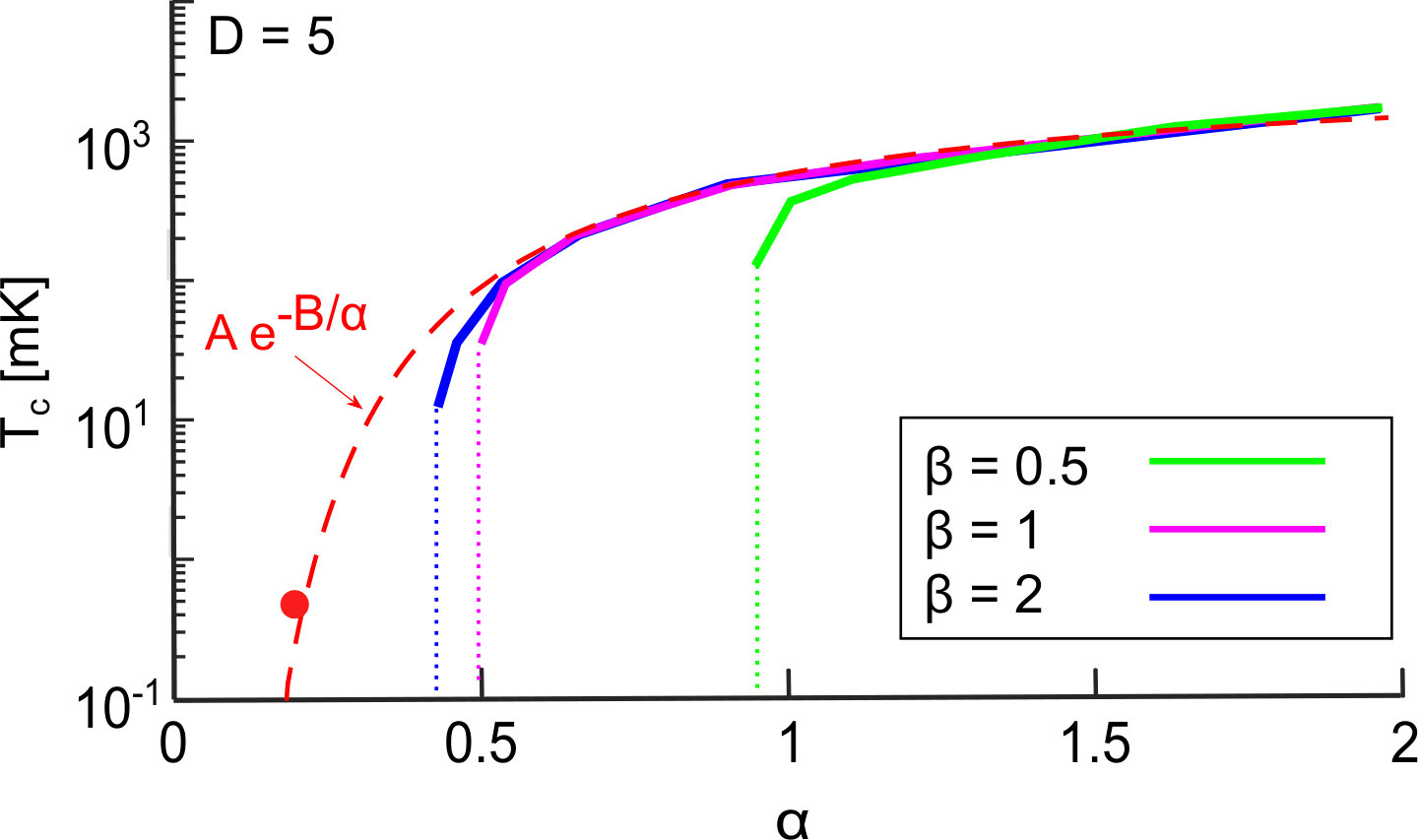 Figure 1
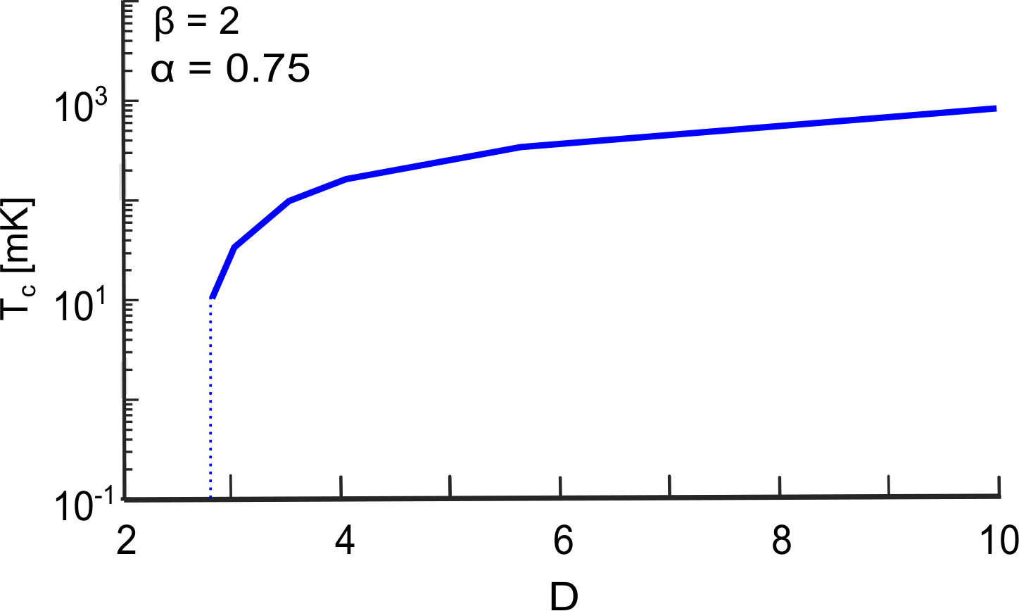 Figure 2
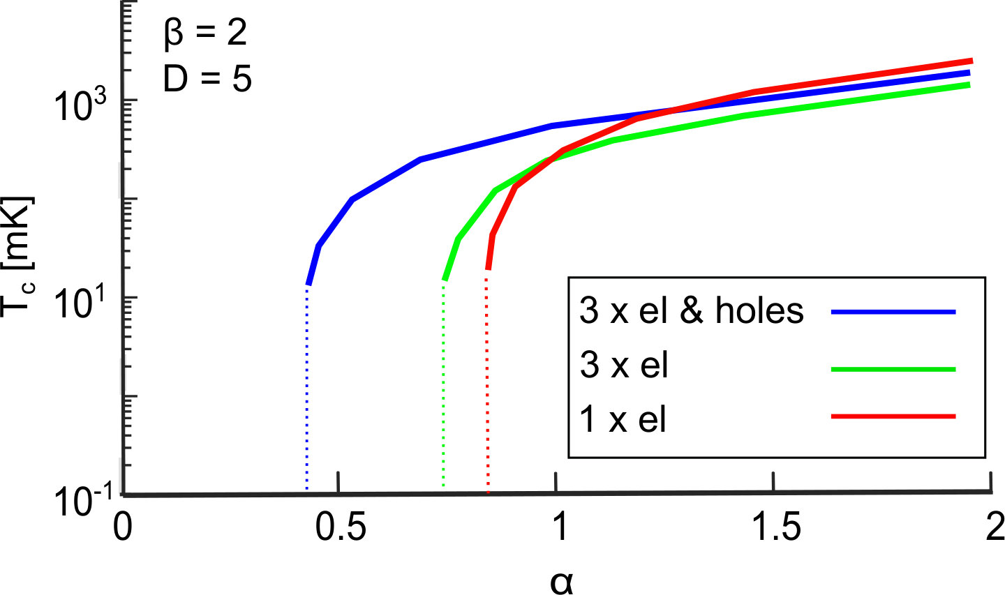 Figure 3
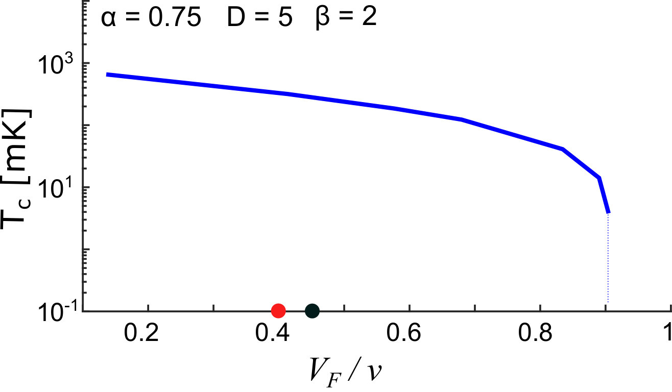 Figure 4
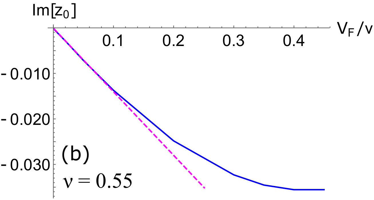 Figure 5
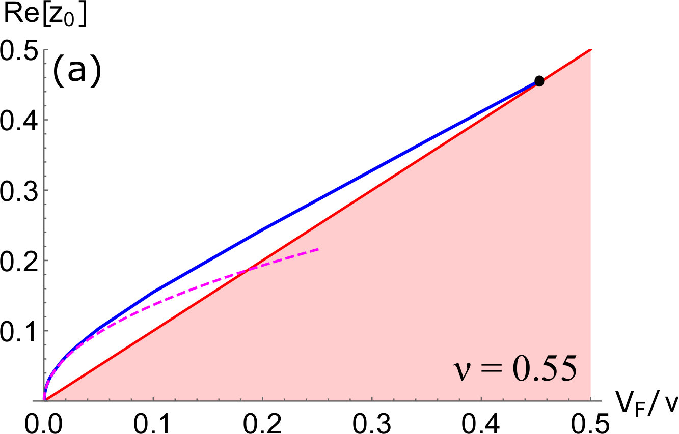 Figure 6
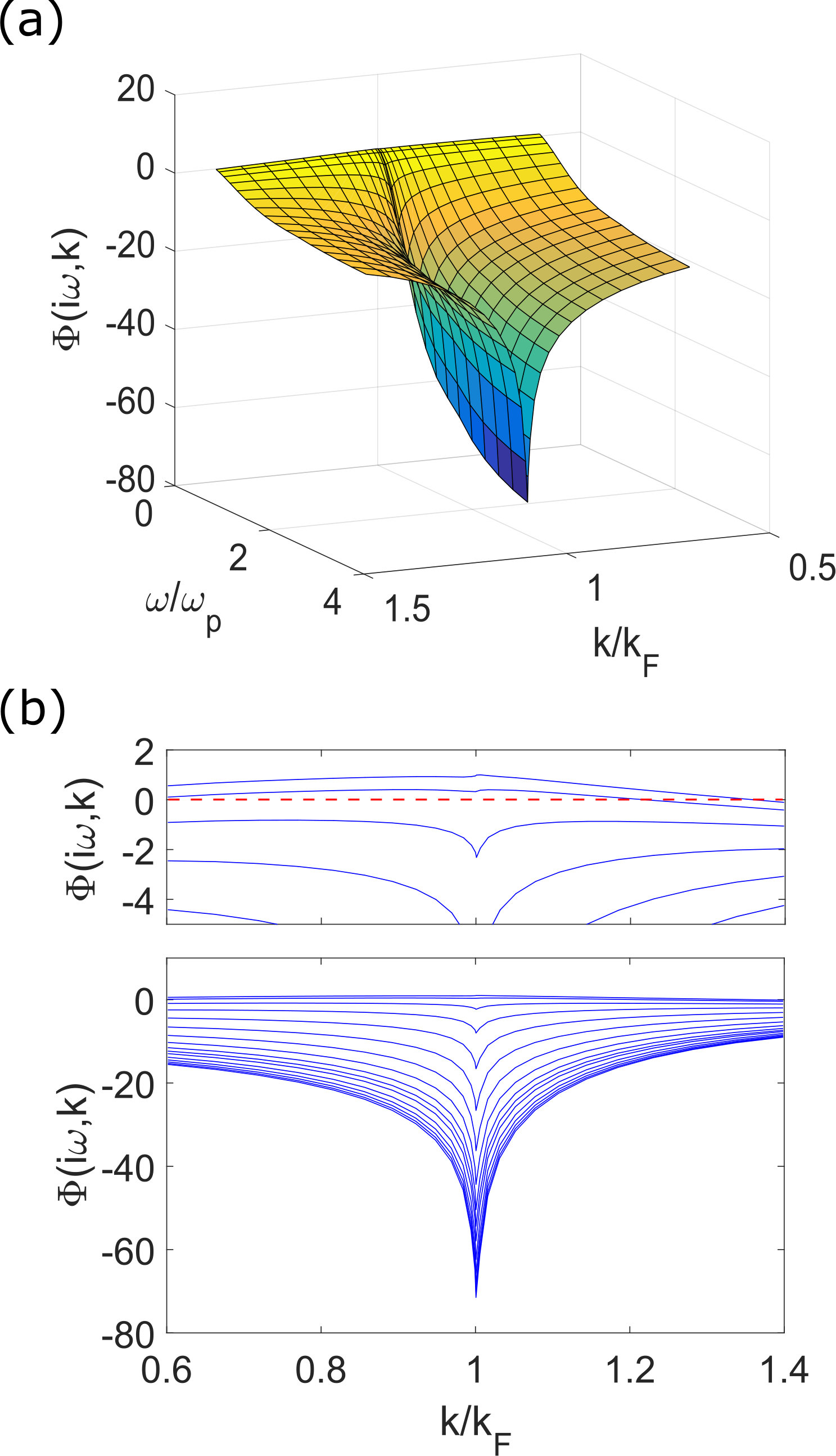 Figure 7
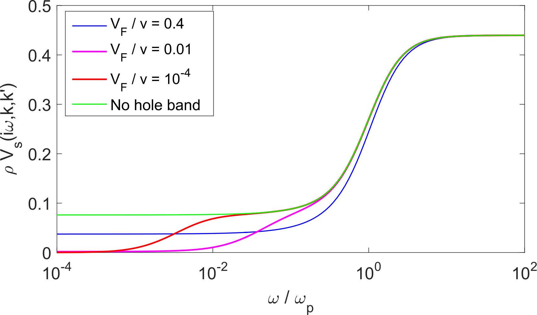 Figure 8
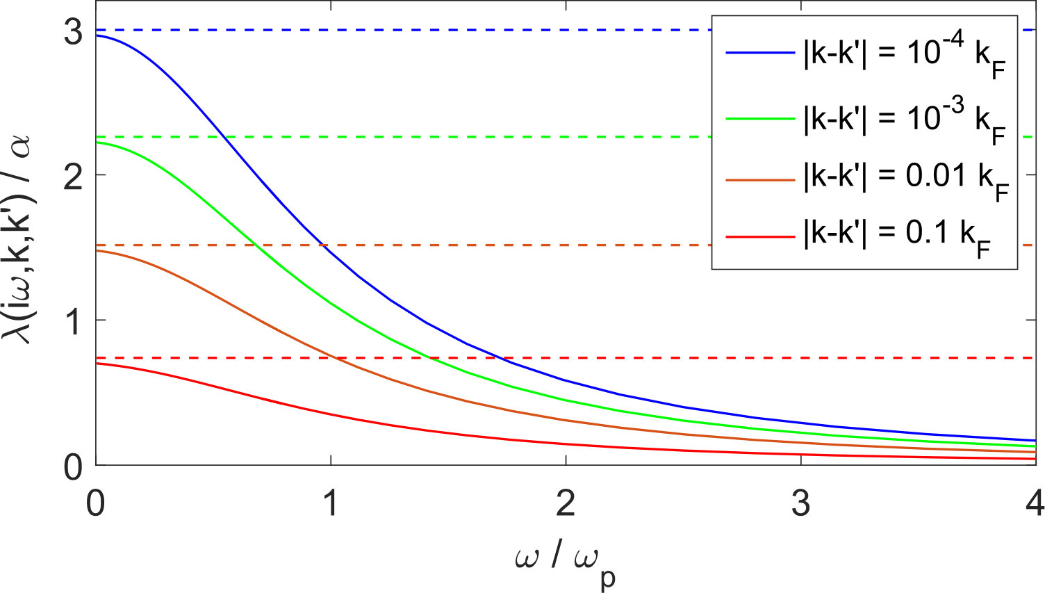 Figure 9
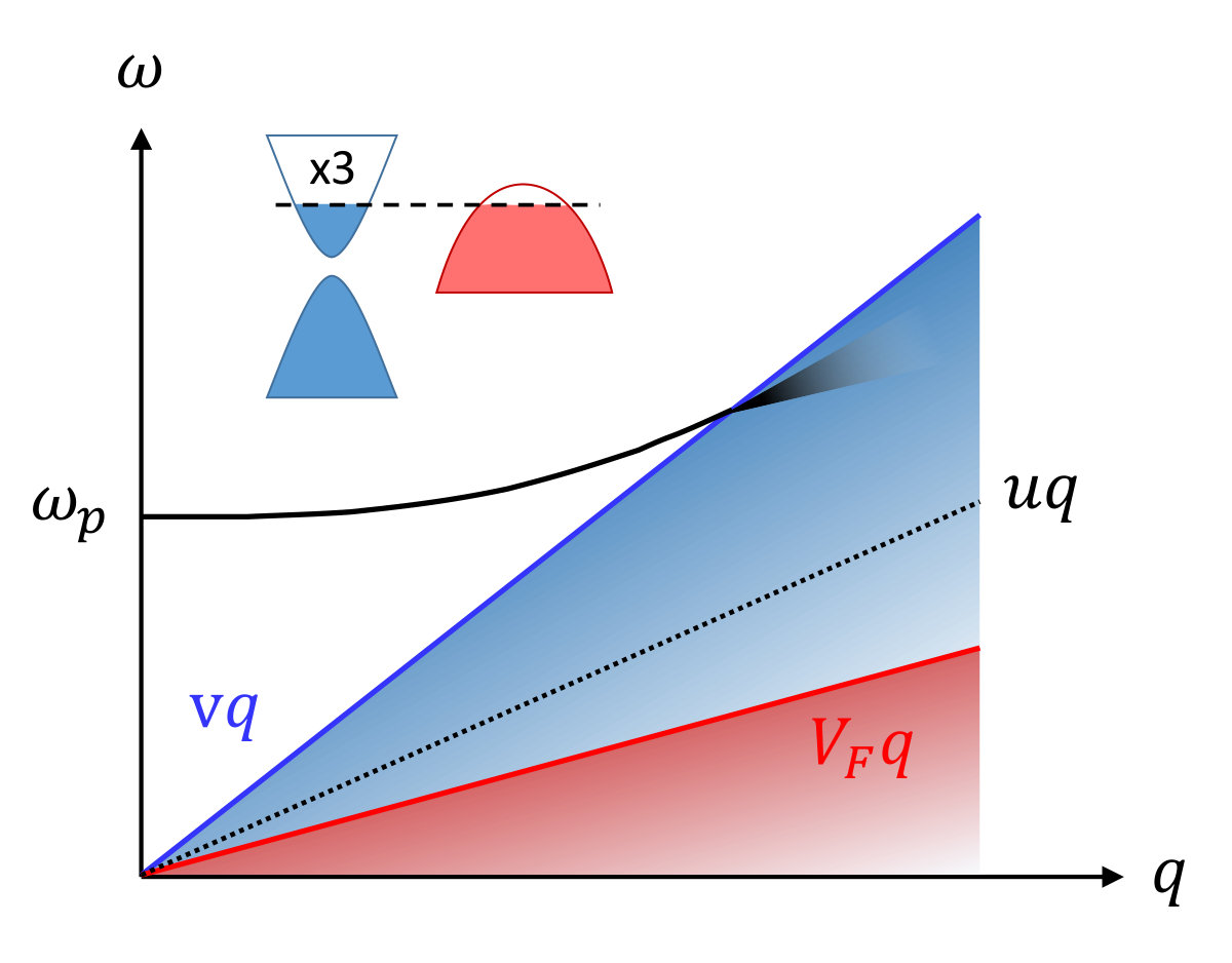 Figure 10
| Parameter | Notation | Value | Reference |
|---|---|---|---|
| Density | Issi (1979); Liu and Allen (1995) | ||
| Total plasma frequency | Tediosi et al. (2007) | ||
| Total Thomas-Fermi momentum | |||
| Static dielectric constant | (isotropic approx.) | see Eq. (8) | |
| Unit cell volume | Liu and Allen (1995) | ||
| Debye temperature | DeSorbo (1958) | ||
| Transition temperature | Prakash et al. (2016) | ||
| Number of electronic pockets | 3 | Issi (1979); Liu and Allen (1995) | |
| Electron Fermi energy | Issi (1979); Liu and Allen (1995); Tediosi et al. (2007) | ||
| Dirac velocities | Issi (1979); Zhu et al. (2011) | ||
| Average electronic velocity | |||
| Dirac mass | Issi (1979); Zhu et al. (2011); Wolff (1964) | ||
| Average electron Fermi momentum | Issi (1979); Zhu et al. (2011) | ||
| Electron density of states (per pocket per spin) | |||
| Electron plasma frequency | |||
| Electron Thomas-Fermi momentum | |||
| Hole Fermi energy | |||
| Hole masses | Liu and Allen (1995); Issi (1979); Zhu et al. (2011) | ||
| Average hole mass | |||
| Average hole Fermi momentum | Issi (1979); Zhu et al. (2011) | ||
| Average hole Fermi velocity | |||
| Hole density of states (per spin) | |||
| Hole plasma frequency | |||
| Hole Thomas-Fermi momentum |
Peer Reviews
No public reviews on file for this paper yet. If you reviewed it on a platform where reviews are public (OpenReview, ICLR, NeurIPS, ICML), you can paste yours below so the community can read it here.
Videos
No videos yet. Explain this paper in a talk, walkthrough, or lecture? Add one.
Taxonomy
TopicsSuperconductivity in MgB2 and Alloys · Physics of Superconductivity and Magnetism · Topological Materials and Phenomena
Pairing from dynamically screened Coulomb repulsion in bismuth
Jonathan Ruhman and Patrick A. Lee
Department of Physics, Massachusetts Institute of Technology, Cambridge, MA 02139 USA
Abstract
Recently, Prakash et. al. have discovered bulk superconductivity in single crystals of bismuth, which is a semi metal with extremely low carrier density. At such low density, we argue that conventional electron-phonon coupling is too weak to be responsible for the binding of electrons into Cooper pairs. We study a dynamically screened Coulomb interaction with effective attraction generated on the scale of the collective plasma modes. We model the electronic states in bismuth to include three Dirac pockets with high velocity and one hole pocket with a significantly smaller velocity. We find a weak coupling instability, which is greatly enhanced by the presence of the hole pocket. Therefore, we argue that bismuth is the first material to exhibit superconductivity driven by retardation effects of Coulomb repulsion alone. By using realistic parameters for bismuth we find that the acoustic plasma mode does not play the central role in pairing. We also discuss a matrix element effect, resulting from the Dirac nature of the conduction band, which may affect in the -wave channel without breaking time-reversal symmetry.
I Introduction
BCS theory explains how superconductivity emerges from a local electron-phonon coupling, and leads to the well known expression for the transition temperature
[TABLE]
Here is the density of states per spin at the Fermi energy, is the Debye temperature and is the phonon mediated interaction. In metals the local electron-phonon coupling is, indeed, the most important one Morel and Anderson (1962).
However, as pointed out first by Gurevich, Larkin and Firsov (GLF) Gurevich et al. (1962), this theory runs into a serious problem when considering superconductivity in dilute metallic systems, such as doped semiconductors and semimetals. The reason is that in three dimensions the density of states, , decreases to zero as the density of carriers is decreased. GLF have concluded that in non-ionic crystals the lowest possible density for superconductivity is 111This density bound, , is obtained by assuming a given band mass . Then is proportional to . Thus, systems with small band masses, such as Bi2Se3, may have a significantly higher bound.. For ionic crystals, on the other hand, they proposed that coupling to the long range polarization of the longitudinal optical phonon, within the random-phase-approximation (RPA), may lead to superconductivity at densities much lower than . It is, however, important to note that the frequency of the longitudinal mode must still be much smaller than the Fermi energy, , such that the Coulomb repulsion may be renormalized.
Indeed, most known superconductors with a density below the limit are ionic compounds 222Although it should be mentioned that the restriction is typically not fulfilled. The extreme example is SrTiO3Schooley et al. (1964); Lin et al. (2013); Chandra et al. (2017), where the phonon frequency is significantly higher than the Fermi energy. But also in the case where the Fermi energy is greater, such as doped PbTe Matsushita et al. (2006), SnTe Sasaki et al. (2012), Bi2Se3 Hor et al. (2010) and the half-Heuslers, the two energy scales are still of the same order of magnitude. Thus, there is an open question regarding how repulsion gets screened, even in the ionic systems.. Examples are the topological half-Heusler semimetals YPtBi, LuPtBi, LaPtBi with densities as low as Butch et al. (2011); Tafti et al. (2013); Nakajima et al. (2015); Kim et al. (2016) and SrTiO3 with a density as low as Schooley et al. (1964); Koonce et al. (1967); Lin et al. (2014, 2013).
The recent discovery of superconductivity in bismuth Prakash et al. (2016), however, is in direct contradiction to the GLF theory. On the one hand the density of carriers, which is , is well below the bound (for a detailed discussion on the irrelevance of phonons and other local interactions to superconductivity see Appendix D). On the other hand bismuth is a single element crystal, and therefore has no polar phonon modes. Thus, the puzzle is: What is the source for long range attractive interaction which allows such a low density system to become superconducting?
The discovery of high- superconductivity has raised the possibility of pairing in lightly doped Mott insulators due to strong correlations effect. However, in Bi the bands are predominantly wide bands and strong correlation is not expected. (For an alternative viewpoint on pairing from strong correlation effects see Ref. Baskaran (2017)). There remain two possible sources for long-ranged attractive interactions: (i) Soft critical fluctuations coming from a nearby critical point (the critical point maybe associated with an instability of the Fermi gas or a structural transition of the ions in the crystal) Metlitski et al. (2015); Lederer et al. (2015); Kozii and Fu (2015); Wang et al. (2016). (ii) The second possibility is collective plasma modes Takada (1978, 1980); Rietschel and Sham (1983); Grabowski and Sham (1984); Takada (1992, 1993), which mediate a long ranged attraction. Since there is no experimental evidence of a nearby critical point we focus, in this paper, on the latter. The plasmonic modes are longitudinal collective modes, which are related to longitudinal phonon modes in a polar crystal. Therefore they are, in principle, compatible with the GLF theory. The plasma modes set the energy scale for the retardation (frequency dependent) effect of the screened Coulomb interaction leading to effective attractive pairing channels.
Takada Takada (1978) was the first to apply the GLF theory to study the possibility of plasmonic superconductivity. He concluded that a superconducting instability can occur if the coupling is strong, i.e. (where is proportional to the ratio between Coulomb interaction and kinetic energies). In this limit the plasma frequency is typically higher than the Fermi energy. Thus, both Eliashberg theory and the RPA are out of their limits of validity. For this reason there has been a lot of controversy in the literature whether or not this instability exists even in theory Rietschel and Sham (1983); Grabowski and Sham (1984); Takada (1993); Grimaldi et al. (1995); Richardson and Ashcroft (1996).
In this work we focus on the limit of weak coupling Ruhman and Lee (2016) where RPA is a good approximation. Our goal is to understand the origin of superconductivity in bismuth, where the measured plasma frequency is smaller than the Fermi energy Tediosi et al. (2007), indicating that indeed . We derive the Eliashberg equation which is used to compute numerically in an isotropic Dirac semi-metal band structure, which approximates that of bismuth. It includes three Dirac-electronic pockets and one parabolic-hole pocket Wolff (1964); Liu and Allen (1995); Zhu et al. (2011), where the Dirac velocity is significantly larger than the Fermi velocity of the holes.
We find, in contrast to Takada Takada (1978, 1992), that there exists a weak coupling instability towards superconductivity and discuss the possibility that this instability extends to arbitrarily weak coupling. By calculating with and without the hole pocket we show that the holes drastically enhances in the weak coupling limit. Our results indicate that Bi may be the first example of weak coupling superconductivity driven by retardation effects of Coulomb repulsion alone, without the help of phonons. We also note that in this case the isotope effect should be completely absent, as the mass of the bismuth atoms plays no role in the theory.
It is also important to note that in the case of bismuth, where there are multiple Fermi surfaces with different Fermi velocities, there may exist an additional collective mode: the so called acoustic plasmon Pines (1956); Ruvalds (1981); Bennacer and Cottey (1989); Bennacer et al. (1989); Chudzinski and Giamarchi (2011). This mode has been considered as a possible mechanism for attractive interactions and superconductivity in semi-metals already a long time ago Garland (1963); Radhakrishnan (1965); Pashitskii (1968); Fröhlich (1968); Ruvalds (1981); Entin-Wohlman and Gutfreund (1984). Such a mode can contribute greatly to superconductivity when the velocity ratio is very large (in this limit the slower band becomes equivalent to the ”jelly” in the ”jellium” model and the acoustic plasmon is just the acoustic phonon). However, we show that for realistic parameters in bismuth a weak coupling instability occurs even in the limit where this mode does not exist, and therefore we argue that the acoustic plasmon is not an essential ingredient for superconductivity in this material. Nevertheless, we find that the hole band tends to enhance the transition temperature.
Finally, in Bi strong spin-orbit coupling leads to nearly massless Dirac conduction bands. Anderson Anderson (1959) pointed out that in the presence of spin-orbit-coupling, one pairs time reversed eigenstates rather than opposite spins, such that the s-wave pairing BCS theory and Eq. (1) remain valid. We find that in the case where the paired states reside on a Dirac cone, this conclusion is violated due to a matrix element effect, as recently found in quadratic band touching semi-metals Savary et al. (2017). For more details see Appendix E.
Contents
II Band structure of Bismuth
We start by quickly reviewing the single particle dispersion of the electron and hole bands. Bismuth has rhombohedral crystal structure, which belongs to the point group symmetry class () Liu and Allen (1995). Strong spin-orbit coupling leads to three electronic pockets centered at the three -points and one hole pocket revolving around the -point. Each one of the electron pockets is descried by a Dirac Hamiltonian Wolff (1964)
[TABLE]
where denotes the direction along the line, and the parameters appear in Table. 1. Here and are Pauli matrices (we use the same notation as Wolff Wolff (1964) for the band notation). Bismuth is time reversal and inversion symmetric. In this basis the symmetries are implemented by and , respectively. The Hamiltonian (2) is diagonalized by the unitary transformation , i.e. . Here .
The hole band is located around the -point (i.e. the trigonal direction). Here the gap between the conduction and valence bands is much larger than the chemical potential, and therefore the dispersion of these carriers is essentially parabolic
[TABLE]
where the z-direction points along the trigonal direction, and Zhu et al. (2011).
The anisotropy in bismuth is fairly large and may have important implications. However, in this work, we will be interested in addressing the puzzles regarding the appearance of superconductivity in bismuth. Thus, for the sake of simplicity, we will approximate the band structure to be isotropic. The isotropic approximation is obtained by considering a mean velocity for the Dirac electrons and a mean mass term for the parabolic holes. This is formally equivalent to redefying the coordinates Zhu et al. (2011) and importantly preserves the density of states at the Fermi level.
The parameters considered in this work for the electron and hole bands appear in Table 1.
III The dynamically screened Coulomb interaction
We consider the effects of the long-ranged Coulomb interaction
[TABLE]
where is a bosonic Matsubara frequency and the dielectric constant is given by
[TABLE]
Here is the static dielectric constant coming, mainly, from low momentum interband transitions. are the intraband polarizations of the electrons and holes, respectively, which are calculated within the random-phase-approximation (RPA) [see Eqs. (28,29) in Appendix A]. Note that here we have neglected the polarization due to interpocket transitions, since it is only important at high momentum.
III.1 Collective modes
As explained, in this paper we focus on the possibility that electronic pairing in bismuth comes from the collective electronic modes, which set the scale of retardation effects and open new pairing channels. The collective modes are given by the zeros of the dielectric function (5). In bismuth there is a significant difference between the Fermi velocity of the holes and electrons. This leads to the appearance of two longitudinal plasma modes Pines (1956); Bennacer and Cottey (1989):
III.1.1 The gapped plasmon
The first pole is the standard plasmon, which describes a collective compression mode of total charge. It is obtained in the limit . In this case both the polarizations of the electrons and the holes in Eq. (5) are in the dynamic regime , where is the total plasma frequency,
[TABLE]
are the plasma frequencies and Thomas-Fermi momenta of the electrons and holes, respectively, is the number of electron pockets, and are the electron and hole density of states per spin and pocket, and . Thus the total plasma frequency, , and the total Thomas-Fermi momentum, can be written as
[TABLE]
The parameter
[TABLE]
is the effective fine structure constant, which appropriately quantifies the coupling strength in a Dirac dispersion. Plugging in the average velocity in Table 1 we find that . The corresponding plasma frequency taken from Eqs. (6 and 7), is given by . To fix the plasma frequency to be equal to the experimental measurement () we set Tediosi et al. (2007), which corresponds to . We note that there is uncertainty in this value because it depends strongly on the assumption of isotropic bands. In reality is estiamted to be higher Boyle and Brailsford (1960) and it is not clear what is the effective coupling strength in the highly anisotropic bands.
The dispersion of the plasmon mode is schematically presented in fig. 1 (solid black line). As can be seen at the mode weakly disperses, until at it crosses into the p-h continuum of the electron pockets (marked by the shaded blue region in the figure) where it becomes over damped. Therefore, there is a limitation on the phase space for scattering by plasmons, which becomes more important at weak coupling, where . The phase space constraint has important implications on superconductivity since it reduces the strength of the attractive interaction coming from the plasmon mode (For more details on the limited phase space of the plasmon see Appendix B).
III.1.2 The acoustic plasmon
The second pole is the acoustic plasmon Pines (1956); Bennacer et al. (1989); Chudzinski and Giamarchi (2011) observed at lower frequency . This mode describes an out-of-phase compression of the two charged fluids, which does not affect any modulation in the total charge. As a result it is neutral and is thus acoustic, similar to the zero sound mode of a neutral Fermi liquid. The main difference compared to a neutral Fermi liquid is, however, that the mode is damped because it lies in the p-h continuum of the electrons.
Here we also point out that in the limit of , the hole serves as positive charge background and the model becomes the ”jellium” model. In this case the acoustic plasmon becomes the sound wave of the jellium liquid Ashcroft and Mermin (1976). The usual BCS theory of the exchange of the acoustic phonon then applies, where the acoustic plasmon takes the place of the phonon. We will see later that Bi is far from this limit.
To obtain the linear dispersion of the acoustic plasmon we seek the zeroes of (5) near which are given by the equation
[TABLE]
where and . The solution of equation (9), denoted by , depends on two parameters: and (see discussion below Eq. (6) for definitions). If there exists a solution it is always in the regime and thus the l.h.s of Eq. (9) contributes a non-trivial imaginary part, which leads to damping of the mode reflected by . The general solution can thus be written as
[TABLE]
where and are real positive numbers.
By solve Eq. (9) numerically we find that there exists a solution of the form (10), however, not for any . Namely, for a given value of there is a , above which, the physical solution of equation (9) disappears. For example, in Fig. 2 we plot the numerical solution of Eq. (9) using the realistic values from Table 1 (giving ). We find that the solution exists only for . Since the realistic parameters in Table 1 correspond to , the acoustic plasmon pole exists within our isotropic approximation, but is close to the critical value for its disappearance. We also find that it is only weakly damped in the whole range where it exists.
To gain more intuition on this mode we can also solve for the acoustic plasmon in the limit of , where the solution gives the known result Bennacer and Cottey (1989)
[TABLE]
This corresponds to the limit of in Fig. 2, where the real part goes to zero like , while the imaginary part goes to zero linearly. We can also obtain the effective electron coupling to the acoustic mode in this limit by expanding the interaction (4) in the vicinity of the mode
[TABLE]
As noted earlier, this gives the same result as in the exchange of acoustic phonons in the jellium model, where the dimensionless coupling constant is given by .
It is important to note that in what follows we do not use the approximate form Eq. (12) to estimate , or in any other place in our calculations. We use the full RPA vertex Eqs. (4, 5) which is dealt with numerically.
IV Superconductivity
We now turn to discuss the possible pairing instabilities due the collective modes of the electronic fluid in bismuth. The frequency of these modes is higher than the corresponding Fermi energy of the holes and therefore we focus on superconducting instabilities driven by the electron pockets, which have a higher Fermi energy. Thus the important role of the hole band in this model comes from its contribution to the RPA polarization (5).
To investigate the instability due to the interaction (4) we utilize the linearized Eliashberg equation (For a detailed derivation see Appendix C)
[TABLE]
where is a matrix representing the order parameter in the two-dimensional basis of occupied bands.
The main difference between standard Eliashberg theory and Eq. (13) is the appearance of the rotation matrices , which project into the band basis of the two occupied bands, and thus adds non-trivial momentum form factors due to spin-orbit coupling. For simplicity, here, we assume -wave pairing, i.e. . In this case, tracing over both sides of Eq. (13) the gap equation assumes the form
[TABLE]
where
[TABLE]
This additional form factor is a consequence of spin-orbit coupling in the Dirac bands and comes from the transformation of the density operator to the Bloch-band basis (see Appendix C).
We also note that the form factor (15) can potentially reduce in the -wave channel without breaking time-reversal symmetry or modifying the density of states at the Fermi level. For more details on this see Appendix E.
IV.1 -wave superconductivity from the dynamically screened Coulomb interaction
Let us now turn to the main focus of the current work and consider the specific case of the screened Coulomb interaction (4). As mentioned we consider, for simplicity, -wave pairing, in which case the linearized Eliashberg equation (13) reduces to the form
[TABLE]
where The value of is obtained by finding an eigenvector of the kernel
[TABLE]
which has unity eigenvalue. Here is the density of states per spin and pocket and
[TABLE]
is the interaction averaged over the solid angle between and [including the form form factor (15) taken in the limit ].
To make a comparison with standard Eliashberg theory (see for example Ref. Margine and Giustino (2013)) we artificially decompose the interaction into two parts (note that we perform the calculation with the full vertex function (18), and this decomposition is only for the sake of discussion) where
[TABLE]
is the instantaneous Coulomb repulsion and
[TABLE]
is the retarded attractive interaction coming from the collective modes of the electron gas. In Fig. 3 we plot the attractive part (solid lines) of the interaction (20) normalized by the fine structure constant for different values of (using the parameters in Table 1. The repulsive part (19), corresponding to the same values of , and also normalized by is plotted for comparison (dashed lines with corresponding colors). Here the integration over solid angle in Eq. (18) is performed numerically.
It is important to note that the total potential (18) is repulsive for any Matsubara frequency . This is the same in the conventional electron-phonon coupling, where it is crucial to renormalize the high-frequency repulsion, , to a much smaller , such that an effective attraction is obtained.
Let us now compare the interaction terms Eqs. (19, 20), which originate from the electronic polarization (5), with the case of phonon mediated interactions. First, we note that the interaction diverges logarithmically as approaches , as opposed to the phonon case where it is typically a constant. Thus, despite the weak coupling constant () the attractive term can reach reasonably high values. This is crucial for superconductivity in the low density limit.
Second, the difference between the repulsion, , and the zero frequency limit of the attraction, , is weakly dependent on and is very small (it is given by the angular average (18) over the statically screened Coulomb interaction). This implies that at small the strength of the retarded attraction coming from is almost as strong as the instantaneous repulsion . In this scenario, even a small renormalization of the instantaneous repulsion at frequencies higher than the plasma frequency is sufficient to generate attraction. On the other hand, as opposed to phonon superconductivity, the plasma frequency, , is of the same order as the Fermi energy, . Thus there is a very small window of energies between and where this renormalization may occur.
It is also important to note that in the weak coupling limit the form form factor (15) suppresses the repulsion (19) more than it does to the attraction (20), and thus contributes to superconductivity. This is because the attractive part is mainly coming form the plasmon pole which exhibits a divergence. It is dominated by small scattering (i.e. ) and, in that limit the matrix element in Eq. (15) becomes unity and does not suppress the coupling constant. On the other hand the screened repulsion coming from larger gets suppressed due to the angular dependence of (15).
IV.2 Details of the numerical solution
We solve Eq. (16) numerically. First we discretize the momentum integral into points , which are distributed around the Fermi momentum. is the high momentum cutoff and is taken to be . We note that the value obtained for is very weakly affected by the value of the momentum cutoff which can also be set to be equal to or smaller than . What is however a crucial parameter is the density of points near the Fermi surface. We control the density of points using a power law distribution of points around
[TABLE]
where is the exponent defining the divergence of the density of points near the ( corresponds to a uniform distribution):
[TABLE]
Here is the density of points. Similarly, we define a set of Matsubara frequencies , where is the lowest Matsubara frequency and the rest of the points are distributed according to
[TABLE]
where is the divergence exponent for the divergence of Matsubara frequencies around zero and defines the cutoff in units of the fermionic Fermi energy.
To obtain the transition temperature we reshape the kernel in Eq. (17) into a and solve for the eigensystem of this matrix Takada (1992). corresponds to the point where the largest positive eigenvalue reaches unity.
In Fig.[4.a] we plot a typical eigenvector obtained from diagonlization of the kernel (17) as a function of frequency and momentum, using , , , , , , and . In the bottom part of Fig.[4.b] we plot the same eigenvector vs. momentum for different frequencies. At high frequency the gap function is negative and changes sign as the frequency is reduced, consistent with Anderson-Morel Morel and Anderson (1962) type picture. However, as pointed out by Takada (e.g. Takada (1992)), in this case the finite-frequency negative part of the solution, is sharply peaked at and is much larger than the positive part at the lowest Matsubara frequency . In the top panel of of Fig.[4.b] we show a closeup of the bottom panel showing that at small frequency the eigenvector becomes positive.
IV.3 The transition temperature
In Fig. 5 we plot the transition temperature, , vs. the fine-structure constant, , for three different values of and . For comparison, the smallest distance between points corresponding to these values of is and , respectively. To generate this plot we used , , , and .
We find that at higher values of , roughly follows an exponential form (The exponential form is plotted for comparison with and , see dashed line). However, at lower values of , sharply drops to zero at a value which depends on the density of points near , . Naively, this implies that there is a minimal for superconductivity. However, since increasing the density of points near , , which is not a physical parameter, enhances the regime where the exponential decay is observed, we argue that it is also possible that the superconducting instability exists for any small . Numerically, however, we can not obtain a solution at an arbitrarily low . Using the values of and , we find that the measured in bismuth is obtained for , which is consistent with our earlier estimate [see discussion below (8)].
Here it is important to compare our results to the work of Takada Takada (1992), which predicts a minimal for superconductivity despite integrating up to a very high cutoff, . The value of corresponds to the smallest density of points that Takada used in his work, which captures accurately the strong coupling limit but not the weak coupling one (as shown in Fig. 5). Therefore we argue that his minimal for superconductivity is an artifact of the density of points that he chose. We also note as opposed to Ref. Takada (1992), here there is also the heavy hole band, which as we shall see, greatly enhances in the weak coupling limit.
Finally, we point out that here we have not used any phenomenological parameter such as the parameter describing the renormalization of the Coulomb repulsion in conventional Eliashberg theory, Margine and Giustino (2013). However, we have used a high energy cutoff . We find that we always need to use (i.e. to integrate to energies higher than ) to find an instability. Since the processes taken into account in the Eliashberg theory (16) are not necessarily the most dominant contributions in this limit, should be regarded as an (implicit) phenomenological parameter, equivalent to . To get a better understanding of its effect on we plot the transition temperature as a function of in Fig. 6. Here we have used , , , and . As can be seen, increasing the cutoff enhances exponentially.
V Discussion
We now turn to discuss the results. In the previous section we have presented evidence for a weak instability. To understand the role of the multiple bands in bismuth on superconductivity we plot the transition temperature, , vs. the fine-structure constant, , for three different cases (see Fig. 7): (i) with three electron pockets and the single hole pocket, (ii) only three electron pockets and (iii) only, a single electron pocket. By comparing the three, we find that in the weak coupling limit the hole band enhances , much more than the multiplicity of electron bands does. On the other hand, for high the transition temperature reduces as we increase the number of bands.
The strong influence of the holes at weak coupling may come from the existence of the additional acoustic plasmon mode Garland (1963); Radhakrishnan (1965); Pashitskii (1968); Fröhlich (1968); Ruvalds (1981); Entin-Wohlman and Gutfreund (1984). To investigate the role of the acoustic plasmon we calculate the dependence of on the velocity ratio in Fig. 8. We find that the transition temperature decreases with increasing . However, as shown in Fig. 2. (a) above a critical value of , the solution of the acoustic plasmon no longer exists. Nonetheless, the dependence of the transition temperature on is smooth, and no special feature is observed at that point. Therefore, we conclude that the acoustic plasmon is not the main driving force in the large enhancement of at weak coupling (shown Fig. 7).
The origin of this large enhancement becomes clear when considering the averaged interaction of (18) in the static limit. In Fig. 9 we plot the interaction (18) for , , and for the case where there is no hole band. As can be seen the main difference between the curves is the saturation value in the static limit, which can be estimated to
[TABLE]
This value monotonically decreases with increasing [defined in Eq. (7)]. Whereas the high frequency limit is the same in all cases. This implies that in all four cases the instantaneous repulsion (19) is the same. On the other hand, by definition, when the the saturation value at low frequency is larger it implies that (20) is smaller. Thus, in the case where there is no hole band the saturation value is higher because the contribution of the hole band to is vanishing, i.e. , which implies that the overall attractive interaction is weaker.
The reason the hole band is so much more effective in this enhancement than the electrons (see Fig. 7) is that at small the holes greatly enhance while almost not modifying the total plasma frequency [see Eq. (6, 7)]. As we have already established, larger , implies greater attraction. However, it is also crucial that the hole band does not enhance the plasma frequency. The reason is that when the plasma frequency is enhanced it reduces the range of frequencies between the cutoff and where the repulsive part (19) can be renormalized.
As mentioned earlier, in the limit the acoustic plasmon becomes the acoustic phonon in the ”jellium” model. We can see clearly the retardation effect below the scale of the acoustic plasmon frequency. Note that for the realistic value of velocity ratio, , no such separation of scales is visible.
V.1 Experimental consequences
So far we have argued that the attractive interaction in bismuth is generated only from the dynamically screened Coulomb interaction. In this section we discuss the experimental consequences of this prediction.
First, we note that the mass of the bismuth atom did not play any role in our theory. Therefore, the observation of any isotope effect will falsify our theory. It is important to note that measuring the isotope effect in bismuth is challenging due to the large atomic mass. The four stable isotopes of bismuth are Bi207, Bi208, Bi209 and Bi210m, which allows a variation of more than in the mass. The accuracy of the measurements is close to this value and hopefully a conclusive measurement can be done.
Another possible effect is the appearance of a resonant spectral feature in the tunneling density of states above the superconducting gap Schrieffer et al. (1963). This is the fingerprint of a resonant plasmon excited by the tunneling electron, and will therefore appear at the plasma frequency Ruhman and Lee (2016) and is expected to change when going through the transition. Such a feature has been observed in optical infra-red reflectivity measurements performed at higher temperatures Tediosi et al. (2007), signaling the strong electron-plasmon coupling in bismuth.
Finally, according to our predictions the density of states of the holes enhances . It would be interesting to see whether the application of uniaxial strain, which enhances the hole mass, can enhance .
VI Conclusions
We have studied superconductivity in Bismuth. We argued that at low carrier concentration only long-ranged interactions are capable of causing such an instability. In the absence of any experimental evidence of a critical point we investigated the more likely scenario in which the dynamically screened Coulomb repulsion gives rise to an effective retarded attraction on the energy scale of the longitudinal plasma oscillations. We used an approximate isotropic band structure and the random phase approximation for the screened Coulomb interaction. Within these approximations we found that there is a weak coupling instability.
The transition temperature is greatly enhanced by the existence of a heavy hole band. We showed that this enhancement is due to the large mass of the holes, which allows for an enhancement of the static screening (Thomas-Fermi) without enhancing the plasma frequency. We showed that is not dramatically decreased when the acoustic plasma mode is absent. Therefore, we concluded that it is not the main contributor to attractive interactions in bismuth.
Interestingly, we found that the superconducting instability found by Takada Takada (1992) can be extended to lower coupling strength by enhancing the density of mesh points near the Fermi surface. However, we still observed a minimal coupling strength for the instability. Thus, an interesting question that remains open, but is much motivated by our study, is whether an instability exists at arbitrarily weak coupling?
In this work we have focused on -wave superconductivity. However, as pointed out by Refs. Takada (1992, 1993); Lederer et al. (2015); Metlitski et al. (2015) when the attractive interaction is long ranged (small scattering) the coupling strength in the higher angular momentum channels is comparable to the -wave channel. In this scenario the symmetry of the order parameter is mainly dictated by the short ranged interactions which are not captured by Eq. (4). Therefore, we conclude that one can not rule pairing of higher angular momentum channels in bismuth.
Another interesting product of our work is that we find that when rotating the band basis to the Dirac bands and projecting to the occupied states an additional form form factor appears in the Eliashberg equation. This form factor aids superconductivity by suppressing the repulsion (19). Interestingly, we have also shown that this factor can affect in the -wave channel without breaking time-reversal symmetry, depending on the ratio between the Dirac energy and the mass gap, . Therefore, the case of a Dirac cone goes beyond what was considered by Anderson in his original theory Anderson (1959) and opens the question, what is the effect of disorder in the Dirac mass, and other Dirac bilinears, on superconductivity in semimetals?
The same Anderson’s theorem, concerning the effect of disorder on , also does not hold in this case because of the strong dependance of the attractive interaction. The reason here is that disorder strongly effects small angle scattering, causing smearing of the scattering amplitude over a wider window of momenta. Thus, even the -wave channel can be significantly affected by chemical potential disorder. Therefore, we point out that the influence of disorder on the transition temperature in plasmonic superconductors is not the same as in conventional superconductivity, and therefore should not be used to infer the symmetry of the gap without further study.
VII Acknowledgments
We thank Srinivasan Ramakrishnan, Lucile Savary, Jorn Venderbos, Inti Sodemann, Yuki Nagai, Brian Skinner and Anshul Kogar for many helpful discussions and for pointing out important papers. We also thank Nandini Trivedi and Andrew Dane for pointing out Ref. Prakash et al. (2016). JR acknowledges a scholarship by the Gordon and Betty Moore Foundation under the EPiQS initiative under grant no. GBMF4303. PAL acknowledges the support of DOE under grant no. FG02-03ER46076.
Appendix A Electron and hole polarizations
In this section we write the explicit formula for the electron and hole polarization appearing in the dielectric function Eq. (5). These polarizations are calculated from the standard formulae
[TABLE]
Note the additional Berry-curvature form factors in . We note that the form factor appearing in the first equations is the same as (15). Neglecting the small band mass, , of the electron pockets, the exact formula for these polarization bubbles is given by
[TABLE]
and
[TABLE]
where , are the density of states per spin and pocket, , , and .
Appendix B Collective modes in a two fluid model
In this section we derive the effective interaction in the vicinity of the collective modes of the electron-hole plasma. In this case, where there are two fluids with significantly different Fermi velocities, there are two fermi-surface volume modes: the gapped plasmon and the acoustic plasmon. These modes are obtained by seeking the zeros of the dielectric function (5), i.e. by solving the equation
[TABLE]
To get an intuitive picture, however, it will be sufficient to focus on the limit of where Eq. (30) reduces to
[TABLE]
where , , and .
B.0.1 The gapped plasmon
The first mode, the gapped plasmon, occurs in the high frequency regime , where the electron and hole polarization are deep in the dynamic limit . Therefore we find a solution of Eq. (31) at where , and . The resulting interaction Eq. (4) assumes the form
[TABLE]
Plugging in realistic parameters for the averaged velocities and Thomas-Fermi momenta, , , and , we find that to match the experimental value of the plasma frequency, , we need . (Note the significant deviation from the measured dielectric constant, Boyle and Brailsford (1960) which is due to the isotropic approximation).
Eq. (32) is known as the plasma pole approximation, which captures the position of the plasma pole in frequency space but not the effective electron-plasmon coupling strength. The main reason for this inaccuracy is that at higher momentum, , the plasmon runs into the p-h continuum of the electron bands and becomes strongly damped (see Fig. 1). Denoting that Gurevich et al. (1962) we can obtain a better approximation for the plasmon coupling by limiting the the phase space of
[TABLE]
where interpolates to the value of the screened Coulomb interaction in the static limit .
From Eq. (33) we see that the plasmon response is observed in a window of scattering angles on the Fermi surface defined by .
B.0.2 The acoustic plasmon
The second mode, the acoustic plasmon, is observed at lower frequencies . This limit lies within the p-h continuum of the electrons (see Fig. 1), which means that the function non-zero imaginary part and therefore we must seek a solution of Eq. (31) in the complex plane Pines (1956); Bennacer and Cottey (1989), such that
[TABLE]
and where and are real positive numbers and where .
In Fig. 2 we plot the numerical solution of the damped pole vs. values the velocity ratio . The shaded region in panel (a) marks the onset of the particle hole continuum of the holes (where ). Thus, in this regime there is no longer a solution. Note that using the parameters in Table 1 we get and .
We find that the acoustic plasmon, for these parameters, is weakly damped. The velocity of this mode increases with . However, for the solution disappears and the only solution of Eq. (31) is the gapped plasmon.
We can also obtain an analytic solution of the acoustic plasmon in the limit of . In this case Eq. (9) assumes the form
[TABLE]
In the limit of small this gives the well known resultBennacer and Cottey (1989)
[TABLE]
Appendix C Eliashberg theory
C.1 The action in Nambu space
As a preparatory step for the Eliashberg theory we transform the Hamiltonian to an action in Nambu space. Comparing the plasma frequency with the Fermi energy of the holes and electrons in bismuth (Table. 1) we find that the plasmon is only retarded with respect to the electrons. Therefore we will focus on the electron pockets here.
C.1.1 Free part
A single Dirac pocket, Eq. (2), is written in Nambu space as
[TABLE]
where the Nambu spinor are given by
[TABLE]
and is written in the notations of Re. Wolff (1964). The Hamiltonian is time-reversal symmetric, and therefore , where . Therefore, the free action Eq. (36) it is diagonalized by the unitary matrix
[TABLE]
Here is the matrix which diagonalizes (i.e. ), , and represent Pauli matrices in Nambu space. The free part of the action, written in the band basis is therefore
[TABLE]
where runs over spin and band basis,
[TABLE]
C.1.2 Interaction part
We now turn to write the Coulomb interaction in the Nambu basis. We start from
[TABLE]
where is total volume.
It is useful to note that the density in Nambu space transforms to the band basis as follows
[TABLE]
where
[TABLE]
Therefore, the interaction assumes the following form when written in the band basis
[TABLE]
where
[TABLE]
is a rank 4 tensor which obeys the equality
[TABLE]
We also note that is an even function of .
C.1.3 Projection to the occupied bands
Since only two bands are occupied in each pocket we restrict the analysis to those bands. In the band basis this a trivial task: We simply restrict the sum over band indices to the hole bands. Therefore they now become indices running over two hole bands which are related to each other by TRS and are denote by .
C.2 Derivation of the gap equation
We now turn to derive the Eliashberg theory for superconductivity due to the interaction Eq. (4). We first introduce the definition of the self-energy
[TABLE]
where is the bare Green’s function in the band basis and is the dressed one. The self energy is then given by
[TABLE]
where the two terms on the r.h.s. of the first line come from two possible contractions of the interaction Eq. (40) with (note that here each one of these contractions can be taken in two equivalent ways due to the fact that we have artificially doubled the the number of fields when going to Nambu space). In the latter diagram one needs to interchange with and with . In the transition to the second line we have used Eq. (42).
For simplicity we will neglect dispersion and mass corrections (These are typically important for extremely accurate calculation of the gap in the limit of intermediate coupling strength). In this case we have
[TABLE]
where .
For simplicity we assume the gap function is well defined under inversion, that is (Note that in Bismuth does ot have inversion symmetry and therefore, in general, one needs to consider a more generic gap function). We can consider two distinct cases: even parity, where and or odd parity, where and . In this case we can write
[TABLE]
where for odd parity and is trivially defined for even parity. Therefore
[TABLE]
C.3 Estimation of the transition temperature
To estimate the transition temperature we linearize Eq. (13), i.e. we neglect the dependence in the denominator. We also consider, for simplicity, a -wave gap function. In this case we have
[TABLE]
Note that here we have normalized the matrices such that . Taking the sum over momentum to an integral and performing the integral over the solid angle we obtain
[TABLE]
where is given by
[TABLE]
Appendix D Ruling out the phonon mechanism for superconductivity
Throughout this paper we have only considered Coulomb interactions, neglecting all possible local interactions. The argument was that the density of states in bismuth is too low, such that local interactions are negligible. In this section we elaborate on this point.
Let us first consider the standard electron-phonon coupling to the longitudinal acoustic phonon considered for conventional superconductors De Gennes (1989)
[TABLE]
where is the dispersion of the phonon branch, is the sound velocity, is the mass density and are the phonon creation and annihilation operators, respectively. is the deformation potential, which is typically of order and in Bismuth has been estimated to be , at most Katsuki (1969). The resulting phonon-mediated interaction in Matsubara space is then given by
[TABLE]
From this, we can estimate the coupling strength by taking the zero frequency limit of the interaction times the density of states in Table 1. We find that
[TABLE]
which corresponds to a transition temperature, , which is much lower than . Since Eq. (50) is independent on we may is also roughly estimates the coupling to the longitudinal optical branches by extrapolating to the zone boundary.
It is important to note two additional factors that reduce the effectiveness of the attractive interaction Eq. (50). First, we did not take into account the matrix element effect Eq. (15), which will further reduce in the electron bands. The second is that we have neglected any repulsion coming from the Coulomb interaction (4), which will be poorly screened in the low density limit and will completely overwhelm the small attraction coming from these phonons.
We also find evidence to rule out the phonon mechanism in bismuth based on recent density functional theory (DFT) calculations Meinert (2016). In this study the author studied superconductivity in YPtBi, which is characterized by a density of and a density of states (Comparing with Table 1 the density of states is comparable to that in bismuth). He ignored the polar nature of the phonons and used a mesh of and for the phonon and electron dispersion, which is clearly too small because the grid must be dense on the scale of , nevertheless he found the coupling constant is . Since the electron phonon coupling in YPtBi is not anomalously small we conclude that these calculations rule out the possibility of non-polar phonon superconductivity at such low density, in agreement with the early results of Ref. Gurevich et al. (1962).
We can also estimate the coupling constant based on the superconducting states observed in amorphus bismuth below Shier and Ginsberg (1966). The electronic density is , thus we estimate the density of states and the phonon mediated interaction to be , where is the unit cell volume. Assuming that the short range physics of the electron phonon coupling does not change dramatically in crystalline bismuth we estimate and . Again, too small to be relevant for superconductivity.
Finally, it is also important to point out that in spite of the very low in bismuth the coupling constant can not be smaller that . Inverting the density of states and assuming a general local interaction of the form
[TABLE]
and taking we find that the phonon mediated interaction must be at least . Thus, when interpreting the attractive interaction in bismuth as local, with a typical crystalline length scale, it takes an unphysically large value indicting that superconductivity does not come from local interactions.
Appendix E Matrix element modifications of the BCS formula for
The additional form factor (15) has an important effect on superconductivity, regardless of the pairing mechanism. To see this, let us consider the constant attractive interaction that BCS considered in their original paper (i.e. Eq.(51), which corresponds to ). Without spin-orbit coupling the matrices become trivial and Eq. (13) reduces to (for -wave pairing)
[TABLE]
where is the electronic density of states per pocket and spin. Note that we have made the assumption . The corresponding transition temperature is given by Eq.(1). In contrary, within the Dirac dispersion, where spin orbit coupling is present, we find two crucial differences:
(i) First we find that the odd parity pairing channel [of the form ], may also have a finite transition temperature in spite of the structureless interaction assumed by BCS. This is contracts to the case of no spin-orbit coupling, where one finds that the transition temperature to an odd-parity state is strictly zero. This origin for this difference is the matrices in Eq. (13) which encode the channel’s parity into non-trivial momentum dependent form factors. Note that for odd-parity pairing is proportional to a sum of the Pauli matrices and therefore the factor (15) takes a different form.
(ii) Second, we find that when averaging (15) over the solid angle between and the second term in the l.h.s. averages to zero. When Eq. (15) gives a factor of reduction of the coupling constant. For finite we find (for -wave pairing)
[TABLE]
Thus, in the parabolic limit the transition temperature reduces to Eq. (1). However, in the relativistic limit the coupling constant is reduced by a factor of and consequently is reduced exponentially. Note that here we have assumed a constant density of states. Thus the parameter continuously tunes between Eq. (1) and the much suppressed transition temperature .
The latter is in sharp contradiction to the conventional wisdom based on Anderson’s Anderson (1959) notion of pairing time reversed states which states that any time-reversal-symmetric perturbation that does not modify the density of states also does not modify the transition temperature. The origin of the contradiction is the projection to the occupied bands, which was not considered as a possibility in Ref. Anderson (1959). Anderson used the completeness of eigen states to prove that the transformation from one eigen basis to the other does not modify the matrix element in the -wave channel. However, the action of projection violates the completeness of the basis and allows to get an overlap smaller than one.
A similar matrix element effect has been discussed in detail in Ref. Savary et al. (2017), where superconductivity in a quadratic band touching point has been considered. It is found that the suppression of the -wave channel is maximal, i.e. the form factor (15) is equal to as long as the band touching point is not gapped. Note that the same applies to Dirac semi-metals, namely in the case of the form factor (15) becomes equal to after angular averaging.
The reference list from the paper itself. Each links out to its DOI / PubMed record.
- 1Morel and Anderson (1962) P. Morel and P. W. Anderson, Phys. Rev. 125 , 1263 (1962) . · doi ↗
- 2Gurevich et al. (1962) L. V. Gurevich, A. I. Larkin, and Y. A. Firsov, Sov. Phys. Sol. State 4 , 131 (1962).
- 3Note (1) This density bound, n G L F subscript 𝑛 𝐺 𝐿 𝐹 n_{GLF} , is obtained by assuming a given band mass m 𝑚 m . Then n G L F subscript 𝑛 𝐺 𝐿 𝐹 n_{GLF} is proportional to n G L F ∝ m − 3 proportional-to subscript 𝑛 𝐺 𝐿 𝐹 superscript 𝑚 3 n_{GLF}\propto m^{-3} . Thus, systems with small band masses, such as Bi 2 Se 3 , may have a significantly higher bound.
- 4Note (2) Although it should be mentioned that the restriction ω L ≪ ϵ F much-less-than subscript 𝜔 𝐿 subscript italic-ϵ 𝐹 {\omega}_{L}\ll{\epsilon}_{F} is typically not fulfilled. The extreme example is Sr Ti O 3 Schooley et al. ( 1964 ); Lin et al. ( 2013 ); Chandra et al. ( 2017 ) , where the phonon frequency is significantly higher than the Fermi energy. But also in the case where the Fermi energy is greater, such as doped Pb Te Matsushita et al. ( 2006 ) , Sn Te Sasaki et al. ( 2
- 5Butch et al. (2011) N. P. Butch, P. Syers, K. Kirshenbaum, A. P. Hope, and J. Paglione, Physical Review B 84 , 220504 (2011).
- 6Tafti et al. (2013) F. Tafti, T. Fujii, A. Juneau-Fecteau, S. R. de Cotret, N. Doiron-Leyraud, A. Asamitsu, and L. Taillefer, Physical Review B 87 , 184504 (2013).
- 7Nakajima et al. (2015) Y. Nakajima, R. Hu, K. Kirshenbaum, A. Hughes, P. Syers, X. Wang, K. Wang, R. Wang, S. R. Saha, D. Pratt, et al. , Science advances 1 , e 1500242 (2015).
- 8Kim et al. (2016) H. Kim, K. Wang, Y. Nakajima, R. Hu, S. Ziemak, P. Syers, L. Wang, H. Hodovanets, J. D. Denlinger, P. M. Brydon, et al. , ar Xiv preprint ar Xiv:1603.03375 (2016).