Generalised Summation-by-Parts Operators and Variable Coefficients
Hendrik Ranocha

TL;DR
This paper introduces new formulations for generalised summation-by-parts (SBP) operators that ensure conservation and stability in high-order numerical methods for conservation laws, overcoming previous limitations related to boundary treatment.
Contribution
The authors propose novel discretisation techniques using generalised SBP operators that maintain conservation and stability, addressing boundary treatment challenges.
Findings
New formulations enable conservative and stable discretisations.
Overcomes boundary treatment issues in generalised SBP operators.
Enhances the robustness of high-order methods for conservation laws.
Abstract
High-order methods for conservation laws can be highly efficient if their stability is ensured. A suitable means mimicking estimates of the continuous level is provided by summation-by-parts (SBP) operators and the weak enforcement of boundary conditions. Recently, there has been an increasing interest in generalised SBP operators both in the finite difference and the discontinuous Galerkin spectral element framework. However, if generalised SBP operators are used, the treatment of the boundaries becomes more difficult since some properties of the continuous level are no longer mimicked discretely --- interpolating the product of two functions will in general result in a value different from the product of the interpolations. Thus, desired properties such as conservation and stability are more difficult to obtain. Here, new formulations are proposed, allowing the creation of…
Click any figure to enlarge with its caption.
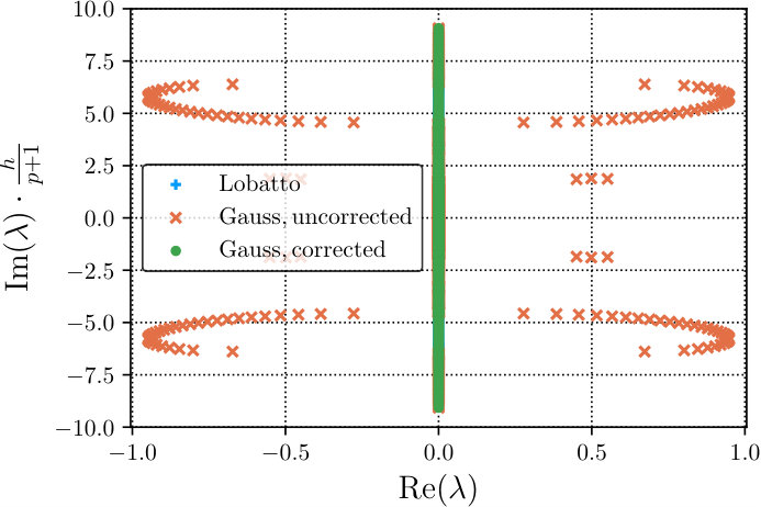 Figure 1
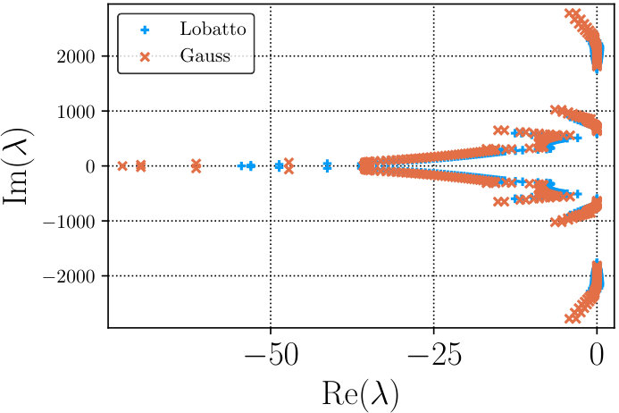 Figure 2
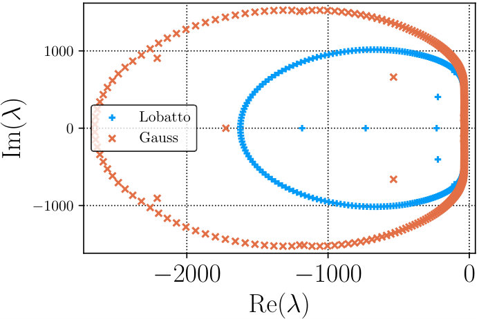 Figure 3
 Figure 4
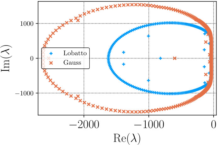 Figure 5
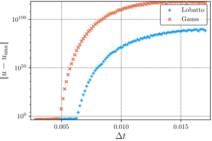 Figure 6
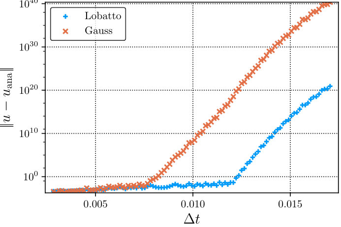 Figure 7
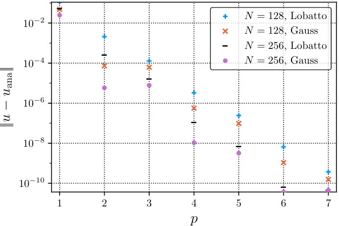 Figure 8
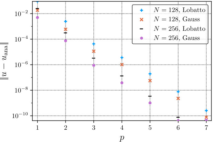 Figure 9
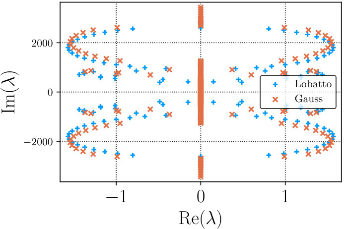 Figure 10
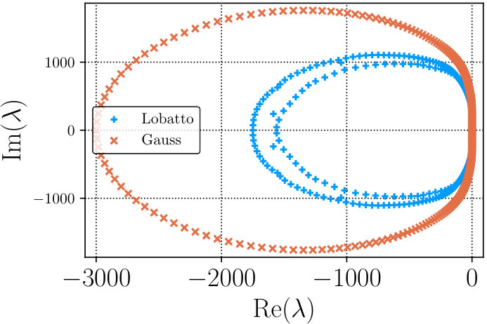 Figure 11
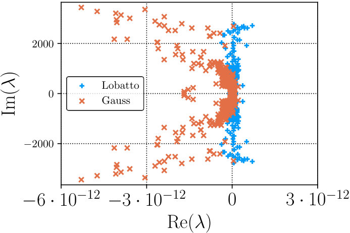 Figure 12
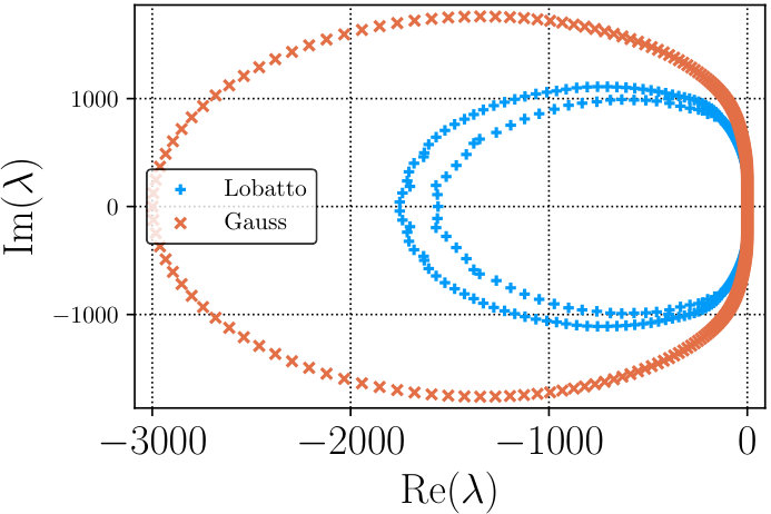 Figure 13
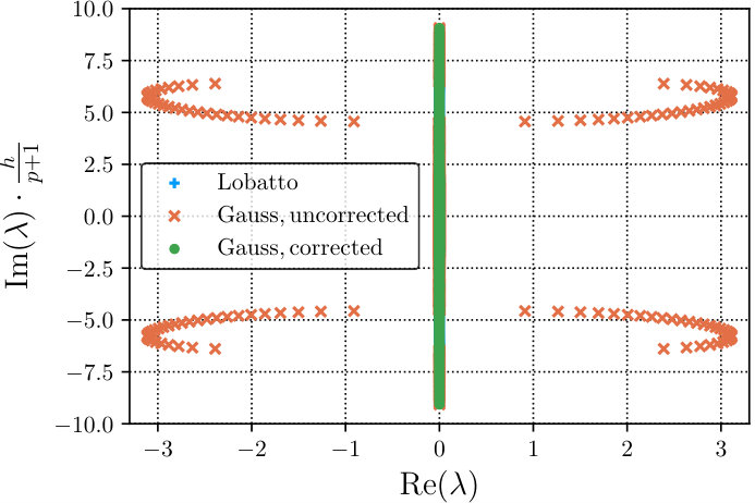 Figure 14
| Split form (31) | Unsplit form (50) | |||||||||
| Central flux | Upwind flux | Central flux | Upwind flux | |||||||
| EOC | EOC | EOC | EOC | |||||||
| Lobatto nodes (Lobatto for ) | 4.05e-02 | 4.06e-02 | 4.24e-02 | 4.25e-02 | ||||||
| 1.16e-03 | 5.13 | 1.18e-03 | 5.10 | 1.08e-03 | 5.29 | 1.11e-03 | 5.26 | |||
| 2.15e-04 | 2.43 | 2.25e-04 | 2.39 | 2.15e-04 | 2.34 | 2.25e-04 | 2.29 | |||
| 8.76e-06 | 4.62 | 8.80e-06 | 4.68 | 8.83e-06 | 4.60 | 8.90e-06 | 4.66 | |||
| 2.42e-07 | 5.17 | 1.94e-07 | 5.51 | 2.45e-07 | 5.17 | 1.96e-07 | 5.50 | |||
| 6.82e-09 | 5.15 | 3.41e-09 | 5.83 | 6.88e-09 | 5.15 | 3.46e-09 | 5.83 | |||
| 4.32e-03 | 4.32e-03 | 4.73e-03 | 4.73e-03 | |||||||
| 8.73e-04 | 2.31 | 8.66e-04 | 2.32 | 8.71e-04 | 2.44 | 8.64e-04 | 2.45 | |||
| 4.16e-05 | 4.39 | 4.13e-05 | 4.39 | 4.22e-05 | 4.37 | 4.19e-05 | 4.37 | |||
| 6.88e-07 | 5.92 | 7.27e-07 | 5.83 | 7.02e-07 | 5.91 | 7.40e-07 | 5.82 | |||
| 6.52e-09 | 6.72 | 7.70e-09 | 6.56 | 6.66e-09 | 6.72 | 7.87e-09 | 6.56 | |||
| 6.35e-11 | 6.68 | 7.59e-11 | 6.66 | 6.45e-11 | 6.69 | 7.72e-11 | 6.67 | |||
| Gauss nodes (Lobatto for ) | 1.36e-02 | 1.35e-02 | 1.53e-02 | 1.53e-02 | ||||||
| 5.30e-04 | 4.68 | 4.89e-04 | 4.79 | 5.77e-04 | 4.73 | 5.27e-04 | 4.86 | |||
| 4.48e-05 | 3.56 | 5.34e-05 | 3.19 | 4.51e-05 | 3.68 | 5.46e-05 | 3.27 | |||
| 2.63e-06 | 4.09 | 2.44e-06 | 4.45 | 2.68e-06 | 4.07 | 2.52e-06 | 4.44 | |||
| 9.71e-08 | 4.76 | 5.62e-08 | 5.44 | 9.88e-08 | 4.76 | 5.82e-08 | 5.44 | |||
| 3.16e-09 | 4.94 | 1.01e-09 | 5.80 | 3.22e-09 | 4.94 | 1.04e-09 | 5.80 | |||
| 3.56e-03 | 3.55e-03 | 3.93e-03 | 3.93e-03 | |||||||
| 1.67e-04 | 4.42 | 1.60e-04 | 4.47 | 1.72e-04 | 4.51 | 1.65e-04 | 4.57 | |||
| 1.06e-05 | 3.98 | 1.06e-05 | 3.92 | 1.11e-05 | 3.95 | 1.11e-05 | 3.90 | |||
| 1.63e-07 | 6.02 | 2.08e-07 | 5.67 | 1.72e-07 | 6.02 | 2.18e-07 | 5.67 | |||
| 1.07e-09 | 7.25 | 2.29e-09 | 6.50 | 1.13e-09 | 7.25 | 2.40e-09 | 6.50 | |||
| 3.65e-11 | 4.88 | 4.14e-11 | 5.79 | 3.65e-11 | 4.95 | 4.19e-11 | 5.84 | |||
| Gauss nodes (Gauss for ) | 1.36e-02 | 1.35e-02 | 1.53e-02 | 1.53e-02 | ||||||
| 5.30e-04 | 4.68 | 4.89e-04 | 4.79 | 5.77e-04 | 4.73 | 5.27e-04 | 4.86 | |||
| 4.48e-05 | 3.56 | 5.34e-05 | 3.19 | 4.51e-05 | 3.68 | 5.46e-05 | 3.27 | |||
| 2.63e-06 | 4.09 | 2.44e-06 | 4.45 | 2.68e-06 | 4.07 | 2.52e-06 | 4.44 | |||
| 9.71e-08 | 4.76 | 5.62e-08 | 5.44 | 9.88e-08 | 4.76 | 5.82e-08 | 5.44 | |||
| 3.16e-09 | 4.94 | 1.01e-09 | 5.80 | 3.22e-09 | 4.94 | 1.04e-09 | 5.80 | |||
| 3.56e-03 | 3.55e-03 | 3.93e-03 | 3.93e-03 | |||||||
| 1.67e-04 | 4.42 | 1.60e-04 | 4.47 | 1.72e-04 | 4.51 | 1.65e-04 | 4.57 | |||
| 1.06e-05 | 3.98 | 1.06e-05 | 3.92 | 1.11e-05 | 3.95 | 1.11e-05 | 3.90 | |||
| 1.63e-07 | 6.02 | 2.08e-07 | 5.67 | 1.72e-07 | 6.02 | 2.18e-07 | 5.67 | |||
| 1.07e-09 | 7.25 | 2.29e-09 | 6.50 | 1.13e-09 | 7.25 | 2.40e-09 | 6.50 | |||
| 3.65e-11 | 4.88 | 4.14e-11 | 5.79 | 3.65e-11 | 4.95 | 4.19e-11 | 5.84 | |||
| Split form (31) | Unsplit form (50) | |||||||||
| Central flux | Upwind flux | Central flux | Upwind flux | |||||||
| EOC | EOC | EOC | EOC | |||||||
| Lobatto nodes (Lobatto for ) | 5.62e-15 | 1.50e-15 | 1.23e-15 | 2.54e-15 | ||||||
| 3.57e-15 | 6.01e-15 | 5.43e-15 | 2.27e-16 | |||||||
| 4.03e-15 | 6.94e-16 | 1.43e-15 | 5.32e-16 | |||||||
| 2.87e-15 | 1.19e-15 | 4.27e-15 | 3.02e-15 | |||||||
| 1.17e-16 | 4.41e-15 | 3.60e-15 | 8.55e-16 | |||||||
| 6.10e-16 | 3.56e-15 | 4.55e-15 | 4.75e-15 | |||||||
| 4.28e-15 | 1.92e-15 | 3.24e-15 | 1.33e-15 | |||||||
| 2.47e-15 | 1.46e-15 | 1.51e-15 | 1.17e-15 | |||||||
| 1.11e-16 | 4.52e-15 | 4.35e-16 | 4.45e-15 | |||||||
| 1.05e-15 | 1.05e-15 | 4.88e-16 | 5.80e-16 | |||||||
| 5.98e-15 | 1.58e-15 | 7.47e-15 | 3.30e-15 | |||||||
| 6.99e-15 | 5.00e-15 | 7.22e-15 | 9.44e-15 | |||||||
| Gauss nodes (Lobatto for ) | 5.41e-16 | 5.31e-15 | 5.34e-04 | 5.36e-04 | ||||||
| 3.91e-15 | 7.92e-15 | 2.26e-05 | 4.56 | 2.27e-05 | 4.56 | |||||
| 9.55e-15 | 6.28e-15 | 7.58e-07 | 4.90 | 7.63e-07 | 4.90 | |||||
| 1.45e-14 | 1.76e-14 | 2.41e-08 | 4.98 | 2.42e-08 | 4.98 | |||||
| 2.41e-14 | 2.12e-14 | 7.55e-10 | 4.99 | 7.60e-10 | 4.99 | |||||
| 5.04e-14 | 5.06e-14 | 2.36e-11 | 5.00 | 2.37e-11 | 5.00 | |||||
| 1.36e-15 | 7.15e-16 | 2.59e-05 | 2.59e-05 | |||||||
| 2.68e-15 | 4.70e-16 | 2.48e-06 | 3.39 | 2.48e-06 | 3.38 | |||||
| 2.60e-15 | 2.29e-15 | 9.56e-08 | 4.70 | 9.56e-08 | 4.70 | |||||
| 4.89e-16 | 4.95e-15 | 3.14e-09 | 4.93 | 3.14e-09 | 4.93 | |||||
| 5.67e-15 | 4.39e-15 | 9.94e-11 | 4.98 | 9.95e-11 | 4.98 | |||||
| 1.42e-14 | 1.40e-14 | 3.12e-12 | 4.99 | 3.12e-12 | 4.99 | |||||
| Gauss nodes (Gauss for ) | 8.41e-07 | 8.41e-07 | 5.34e-04 | 5.35e-04 | ||||||
| 2.64e-08 | 5.00 | 2.64e-08 | 5.00 | 2.26e-05 | 4.56 | 2.27e-05 | 4.56 | |||
| 8.25e-10 | 5.00 | 8.25e-10 | 5.00 | 7.57e-07 | 4.90 | 7.62e-07 | 4.90 | |||
| 2.58e-11 | 5.00 | 2.58e-11 | 5.00 | 2.40e-08 | 4.98 | 2.42e-08 | 4.98 | |||
| 8.32e-13 | 4.95 | 8.33e-13 | 4.95 | 7.54e-10 | 4.99 | 7.59e-10 | 4.99 | |||
| 8.04e-14 | 3.37 | 8.84e-14 | 3.24 | 2.35e-11 | 5.00 | 2.37e-11 | 5.00 | |||
| 1.16e-07 | 1.16e-07 | 2.58e-05 | 2.58e-05 | |||||||
| 3.65e-09 | 4.98 | 3.65e-09 | 4.98 | 2.48e-06 | 3.38 | 2.48e-06 | 3.38 | |||
| 1.14e-10 | 5.00 | 1.14e-10 | 5.00 | 9.55e-08 | 4.70 | 9.55e-08 | 4.70 | |||
| 3.58e-12 | 5.00 | 3.58e-12 | 5.00 | 3.14e-09 | 4.93 | 3.14e-09 | 4.93 | |||
| 1.16e-13 | 4.94 | 1.10e-13 | 5.02 | 9.93e-11 | 4.98 | 9.94e-11 | 4.98 | |||
| 1.05e-14 | 3.46 | 9.88e-15 | 3.48 | 3.13e-12 | 4.99 | 3.12e-12 | 4.99 | |||
| Maximal stable | ||||||
|---|---|---|---|---|---|---|
| Split form (31) | Unsplit form (50) | |||||
| Central flux | Upwind flux | Central flux | Upwind flux | |||
| Lobatto nodes (Lobatto for ) | 3.3 | 5.3 | 3.3 | 5.3 | ||
| 3.1 | 5.2 | 3.1 | 5.2 | |||
| 3.1 | 5.0 | 3.1 | 5.0 | |||
| 3.0 | 5.0 | 3.0 | 5.0 | |||
| 2.6 | 4.6 | 2.6 | 4.6 | |||
| 2.6 | 4.5 | 2.6 | 4.5 | |||
| 2.5 | 4.4 | 2.5 | 4.4 | |||
| 2.5 | 4.3 | 2.5 | 4.3 | |||
| 2.2 | 4.3 | 2.2 | 4.3 | |||
| 2.1 | 4.1 | 2.1 | 4.1 | |||
| 2.1 | 4.0 | 2.1 | 4.0 | |||
| 2.1 | 4.0 | 2.1 | 4.0 | |||
| 1.9 | 4.0 | 1.9 | 4.0 | |||
| 1.8 | 3.9 | 1.8 | 3.9 | |||
| 1.8 | 3.8 | 1.8 | 3.8 | |||
| 1.8 | 3.7 | 1.8 | 3.7 | |||
| 1.6 | 3.8 | 1.6 | 3.8 | |||
| 1.6 | 3.7 | 1.6 | 3.7 | |||
| 1.6 | 3.6 | 1.6 | 3.6 | |||
| 1.6 | 3.5 | 1.6 | 3.5 | |||
| Gauss nodes (Lobatto for ) | 2.3 | 3.4 | 2.3 | 3.4 | ||
| 2.2 | 3.3 | 2.2 | 3.3 | |||
| 2.1 | 3.1 | 2.1 | 3.1 | |||
| 2.1 | 3.1 | 2.1 | 3.1 | |||
| 2.0 | 3.0 | 2.0 | 3.0 | |||
| 1.9 | 3.0 | 1.9 | 3.0 | |||
| 1.8 | 2.9 | 1.8 | 2.9 | |||
| 1.8 | 2.8 | 1.8 | 2.7 | |||
| 1.7 | 2.8 | 1.7 | 2.8 | |||
| 1.6 | 2.7 | 1.6 | 2.7 | |||
| 1.6 | 2.6 | 1.6 | 2.6 | |||
| 1.6 | 2.5 | 1.6 | 2.5 | |||
| 1.5 | 2.5 | 1.5 | 2.5 | |||
| 1.4 | 2.5 | 1.4 | 2.5 | |||
| 1.4 | 2.4 | 1.4 | 2.4 | |||
| 1.4 | 2.3 | 1.4 | 2.3 | |||
| 1.4 | 2.4 | 1.4 | 2.4 | |||
| 1.3 | 2.3 | 1.3 | 2.3 | |||
| 1.3 | 2.3 | 1.3 | 2.3 | |||
| 1.3 | 2.1 | 1.3 | 2.1 | |||
| Lobatto nodes | Gauss nodes | ||||
|---|---|---|---|---|---|
| EOC | EOC | ||||
| 4.89e-03 | 3.16e-04 | ||||
| 1.44e-03 | 1.77 | 8.45e-05 | 1.90 | ||
| 3.04e-04 | 2.24 | 2.20e-05 | 1.94 | ||
| 5.39e-05 | 2.49 | 2.78e-06 | 2.99 | ||
| 9.29e-06 | 2.54 | 5.30e-07 | 2.39 | ||
| 1.47e-06 | 2.66 | 8.77e-08 | 2.60 | ||
| 1.08e-03 | 8.84e-05 | ||||
| 1.48e-04 | 2.86 | 3.08e-05 | 1.52 | ||
| 2.08e-05 | 2.83 | 1.57e-06 | 4.29 | ||
| 4.84e-06 | 2.10 | 2.54e-07 | 2.63 | ||
| 5.75e-07 | 3.07 | 2.91e-08 | 3.13 | ||
| 5.90e-08 | 3.29 | 2.19e-09 | 3.73 | ||
| 2.15e-04 | 7.55e-05 | ||||
| 4.38e-05 | 2.29 | 7.47e-06 | 3.34 | ||
| 7.83e-06 | 2.48 | 1.81e-07 | 5.37 | ||
| 4.54e-07 | 4.11 | 2.52e-08 | 2.85 | ||
| 1.82e-08 | 4.64 | 8.43e-10 | 4.90 | ||
| 7.74e-10 | 4.55 | 3.64e-11 | 4.53 | ||
| 8.42e-05 | 3.84e-05 | ||||
| 1.93e-05 | 2.12 | 6.93e-07 | 5.79 | ||
| 8.98e-07 | 4.43 | 7.63e-08 | 3.18 | ||
| 1.88e-08 | 5.58 | 1.12e-09 | 6.09 | ||
| 1.14e-09 | 4.04 | 5.23e-11 | 4.42 | ||
| 3.17e-11 | 5.17 | 1.18e-12 | 5.47 | ||
| Notation of this article | Finite difference notation | |
|---|---|---|
| Numerical solution | ||
| Multiplication operator | , | , |
| Mass / norm matrix | ||
| Derivative matrix | ||
| Restriction matrix | ||
| SBP property | , , | |
| Correction matrix |
| Notation of this article | DGSEM notation | |
|---|---|---|
| Polynomial degree | ||
| Numerical functions | , | , |
| Multiplication operator | ||
| Discrete product | , | |
| Derivative matrix | ||
| Mass matrix | ||
| Discrete scalar product | , | |
| SBP property | ||
| Numerical flux |
Peer Reviews
No public reviews on file for this paper yet. If you reviewed it on a platform where reviews are public (OpenReview, ICLR, NeurIPS, ICML), you can paste yours below so the community can read it here.
Videos
No videos yet. Explain this paper in a talk, walkthrough, or lecture? Add one.
\titlehead
Generalised Summation-by-Parts Operators and Variable Coefficients
Hendrik Ranocha
(14th November 2017)
Abstract
High-order methods for conservation laws can be highly efficient if their stability is ensured. A suitable means mimicking estimates of the continuous level is provided by summation-by-parts (SBP) operators and the weak enforcement of boundary conditions. Recently, there has been an increasing interest in generalised SBP operators both in the finite difference and the discontinuous Galerkin spectral element framework. However, if generalised SBP operators are used, the treatment of the boundaries becomes more difficult since some properties of the continuous level are no longer mimicked discretely — interpolating the product of two functions will in general result in a value different from the product of the interpolations. Thus, desired properties such as conservation and stability are more difficult to obtain. Here, new formulations are proposed, allowing the creation of discretisations using general SBP operators that are both conservative and stable. Thus, several shortcomings that might be attributed to generalised SBP operators are overcome (cf. J. Nordström and A. A. Ruggiu, “On Conservation and Stability Properties for Summation-By-Parts Schemes”, Journal of Computational Physics 344 (2017), pp. 451–464, and J. Manzanero, G. Rubio, E. Ferrer, E. Valero and D. A. Kopriva, “Insights on aliasing driven instabilities for advection equations with application to Gauss-Lobatto discontinuous Galerkin methods”, Journal of Scientific Computing (2017), https://doi.org/10.1007/s10915-017-0585-6).
1 Introduction
Considering the solution of hyperbolic partial differential equations (PDEs), high order methods can be very efficient, providing accurate numerical solutions with relatively low computational effort [41]. In order to make use of this accuracy, stability has to be established. Mimicking estimates on the continuous level for the PDE via integration-by-parts, summation-by-parts (SBP) operators [42, 74] can be used. In short, SBP operators are discrete derivative operators equipped with a compatible quadrature providing a discrete analogue of the norm. The compatibility of discrete integration and differentiation mimics integration-by-parts on a discrete level. Combined with the weak enforcement of boundary conditions via simultaneous approximation terms (SATs) [8], highly efficient and stable semidiscretisations can be obtained, as described also in [12, 76, 57, 28] and references cited therein.
During the last years, there has been an enduring and increasing interest in the basic ideas of SBP operators and their application in various frameworks including finite volume (FV) [56, 58], discontinuous Galerkin (DG) [19, 18, 38, 21, 62], and the recent flux reconstruction / correction procedure via reconstruction framework [33, 83, 80, 34, 86, 81] as described in [70].
While a mesh of equidistant nodes including the boundaries of the domain is classically used in finite difference methods, multiple elements and nonuniform point distributions possibly not including the boundary nodes are used in discontinuous Galerkin and flux reconstruction schemes. However, the discrete differentiation and quadrature rules can still be compatible, mimicking integration-by-parts. In this context, the notion of generalised summation-by-parts operators [11] covers many stable semidiscretisations and also operators on unstructured meshes in multiple space dimensions [30]. Moreover, using the framework of entropy stable numerical fluxes of [79, 78], entropy stable semidiscretisations can be constructed for systems of nonlinear conservation laws [13, 7, 64, 87, 22, 85, 68, 66]. These methods can be interpreted as generalisations of split forms of the underlying PDE. For classical SBP operators in finite difference methods, these split forms are well known to have desirable conservation and stability properties [54, 14].
However, if generalised SBP operators are used, several problems have to be handled for non-diagonal norms [75] and nodal bases not including boundary nodes, as can be seen in recent investigations by [59] and [47]. In order to remedy these problems, corrections for generalised SBP operators will be presented in this article, extending the work of [67, 69].
Therefore, the article is structured as follows. In section 2, the concept of summation-by-parts operators and generalised SBP operators is introduced. Afterwards, a conservation law with variable coefficients, introducing aliasing issues, is studied in section 3 using the framework of [59]. Introducing new corrections, generalised SBP operators are proven to be both conservative and stable. Similarly, the weighted framework of [47] is applied in section 4, yielding new conservative and stable discretisations using general SBP operators. Thereafter, numerical results for the new methods are presented in section 5, including convergence studies and eigenvalue analyses. Finally, some conclusions are presented in section 7. Moreover, since the notations used in the finite difference and finite element framework are sufficiently different, some translation rules and comparisons with previous works are provided in the appendix.
2 Summation-by-Parts Operators
In this section, a general notion of summation-by-parts (SBP) operators for semidiscretisations of conservation laws will be presented using the notation of [70, 69]. Tables containing translations to the notations used in the finite difference community [59] and the finite element framework [47] can be found in A.
2.1 General Setting
In order to discretise a scalar conservation law in one dimension
[TABLE]
equipped with appropriate initial and boundary conditions, the domain is partitioned into several intervals , where . On each element , the numerical solution is a vector, represented in some finite-dimensional basis by . In finite difference (FD) and nodal discontinuous Galerkin (DG) methods, nodal bases are used, i.e. the representation is given by the values of at pairwise different points . Other choices are also possible, e.g. modal bases [67, 69].
With respect to the chosen basis, (an approximation of) the derivative is represented by the matrix . Moreover, a discrete scalar product is represented by the symmetric and positive definite mass / norm matrix , approximating the scalar product, i.e.
[TABLE]
Additionally, a restriction operator is represented by the matrix , approximating the interpolation of a function to the boundary points . Furthermore, the diagonal boundary matrix gives the difference of boundary values, i.e.
[TABLE]
Finally, these operators fulfil the summation-by-parts property
[TABLE]
mimicking integration-by-parts via
[TABLE]
If linear equations with constant coefficients are considered, these operators suffice to describe appropriate semidiscretisations. For varying coefficients or nonlinear equations, additional multiplication operators have to be used. If the function is represented by , the discrete multiplication operator approximating the linear operator is represented by the matrix , mapping to .
In a nodal basis, the standard multiplication operators consider pointwise multiplication, i.e. they are diagonal . In modal bases, exact multiplication followed by an projection can be considered [67, 69].
2.2 Analytical Setting
In nodal DG methods, the numerical solution is represented as a polynomial of degree on each element. Thus, the matrices can be computed such that they represent the corresponding operations exactly and the SBP property (4) will be fulfilled since it is exactly given by integration-by-parts.
However, the exactness of the mass matrix can be relaxed, since only products of one polynomial of degree and another polynomial of degree are integrated in (5). Considering nodal bases with diagonal mass matrices , a corresponding quadrature rule is given by the positive weights . Thus, the SBP property (4) is fulfilled, if the quadrature given by is exact for polynomials of degree , i.e. Gauss-Lobatto, Gauss-Radau, or Gauss quadrature, since these are exact for polynomials of degree , , and , respectively [39, 31].
2.3 Numerical Setting
There are classical finite difference operators that can be interpreted in an analytical setting similar to the one described above [19]. However, in general — to the authors knowledge — it is not known whether finite difference SBP operators correspond to an analytical basis. Nevertheless, the basic requirement of the SBP property (4) can be enhanced by accuracy conditions in order to get a useful definition of (numerical) SBP operators, cf. [11, 59].
Definition 1**.**
Using a numerical representation of a function in a nodal basis, the operators , and described above form a th order SBP discretisation, if
the derivative matrix is exact for polynomials of degree , 2. 2.
the mass / norm matrix is symmetric and positive definite, 3. 3.
the SBP property (4) is fulfilled, and 4. 4.
\underline{u}^{T}\underline{\underline{R}}{{}^{T}}\underline{\underline{B}}\,\underline{\underline{R}}\,\underline{v}=u\,v\big{|}_{x_{i-1}}^{x_{i}} is exact for polynomials with degrees , where .
These kind of SBP semidiscretisations together with diagonal multiplication operators will be considered in the following. However, modal bases can be used as well [67, 69].
2.4 Special Classes of SBP Discretisations
There are several properties of some SBP discretisations that should be considered separately since they yield special simplifications.
2.4.1 Diagonal Norms Versus Non-Diagonal Norms
If the nodal basis is equipped with a diagonal mass matrix , the positive weights correspond to a quadrature rule, cf. [31]. Moreover, the multiplication operators commute with the mass matrix, since both are diagonal. Thus, multiplication operators are self-adjoint with respect to the scalar product induced by , similarly to multiplication operators in the continuous setting (if the correct domain is chosen). This exact mimicking of properties at the discrete level is desirable, allowing proofs of semidiscrete results analogously to the continuous counterparts.
However, corrections are sometimes possible, if multiplication operators are not self-adjoint. In this case, the -adjoint operator
[TABLE]
can be used to construct appropriate corrections [67, 69, 68]. This has to be used since the discrete multiplication operators are not exact.
2.4.2 Inclusion of Boundary Nodes Versus Bases Exclusion of Boundary Nodes
Another useful property of SBP discretisations is the inclusion of the boundary points into the nodes of the basis. In this case, the restriction operators are simply
[TABLE]
Thus, restriction to the boundary and multiplication commute, i.e.
[TABLE]
This property is fulfilled at the continuous level and therefore also desirable for the semidiscretisation. If the boundary nodes are not included, restriction and multiplication will in general not commute. In this case, some corrections can be applied, e.g. the application of a linear combination of and in order to get the desired results [67, 69, 68]. Again, the reason for this is the inexactness of discrete multiplication operators. However, the construction of correction terms can become cumbersome. In other situations, it might be unknown whether suitable correction terms can be found [66].
2.5 Simultaneous Approximation Terms and Numerical Fluxes
In order to enforce boundary conditions either between neighbouring elements or at the physical boundary of the domain, several methods can be applied. For finite difference methods, these include the injection method (combining the boundary and differential operators directly), the projection method and the usage of simultaneous approximation terms (SATs) [60, 61, 48]. In discontinuous Galerkin methods, boundary conditions are usually enforced via numerical fluxes, resulting in stable schemes. For linear problems, the weak enforcement of boundary conditions via numerical fluxes is equivalent to the use of SATs, as will be shown for the examples in the following sections.
For a conservation law \partial_{t}u(t,x)+\partial_{x}f\big{(}u(t,x)\big{)}=0 with flux not depending explicitly on space and time, a (two-point) numerical flux will be considered to be a Lipschitz continuous mapping consistent with the continuous flux of the conservation law, i.e. , as common in conservative finite difference and finite volume methods, see e.g. [46, 45].
In methods using numerical fluxes , these fluxes are evaluated at the boundaries between two cells. In order to introduce the notation, consider two one-dimensional cells and . On each cell , the numerical solution has a value at the left and right hand side of this cell, written as and , respectively. At the boundary between the cells and , there are two values of the numerical solutions from the neighbouring cells, i.e. and . Here, the indices and refer to values computed from the left and right of a given boundary, respectively. Thus, the numerical flux between the cells and is evaluated as f^{\mathrm{num}}=f^{\mathrm{num}}(u_{-},u_{+})=f^{\mathrm{num}}\Big{(}u^{(i-1)}_{R},u^{(i)}_{L}\Big{)}, as visualised in Figure 1. Finally, the two numerical fluxes and at the left and right hand side of a cell are written as components of the vector .
In the following sections, the linear advection equation with variable coefficients
[TABLE]
with variable speed and compatible initial and boundary conditions , will be considered. Since the flux depends explicitly on the space coordinate via the variable coefficients , the notion of numerical fluxes has to be adapted correspondingly. There are at least two possibilities concerning the evaluation of the variable coefficients:
- i)
Use the speed evaluated at the position of the boundary where the numerical flux is evaluated. 2. ii)
Use some interpolation of the discretised function in the numerical flux.
If boundary nodes are included and the coefficients of the discrete version of the function are obtained by evaluating at these nodes, both possibilities are identical. However, if boundary nodes are not included, the two approaches are different. Moreover, there are several possible versions of the interpolations that can be used. In the remaining sections, the following numerical fluxes for (9) will be considered:
[TABLE]
Here, is the product of the interpolated values of and from the cell on the left hand side. Similarly, is the interpolated value of the product . In the edge based fluxes, the velocity is evaluated at the position of the boundary. In the edge based numerical fluxes (10) and (13), the possibility i) from above is used. The split and unsplit fluxes use possibility ii) with two different choices of the interpolation.
In order to help the reader avoid misunderstandings on the notation, some translation rules to the finite difference setting of [59] and the discontinuous Galerkin spectral element framework of [38, 47] are presented in A.
3 Standard Estimates
In this section, the standard (i.e. unweighted) estimates of [59] will be reviewed and suitable formulations for general SBP discretisations will be presented, resulting in both conservative and stable methods.
3.1 Continuous Setting
Consider the linear advection equation (9) with variable speed and compatible initial and boundary conditions , . The desired properties of this model problem are conservation and stability [59, Section 2]. In order to investigate conservation, the rate of change of the total mass of can be expressed as
[TABLE]
Thus, the change of the total mass is given by the flux through the boundaries.
Similarly, to study stability, the standard estimate can be obtained by application of the product rule and integration by parts
[TABLE]
Thus, if is bounded, the energy estimate
[TABLE]
follows, cf. [59, Section 2]. Hence, in the rest of this section, will be assumed.
Remark 2**.**
In order to enable the above computations, it suffices to consider a speed that is positive at the boundaries . If the speed is positive everywhere, similar properties hold on subintervals of — corresponding to multi-block or multi-element discretisations.
In order to simplify the following investigations, is assumed to be positive everywhere. The case of negative speed or speed with varying sign can be handled analogously. If is negative at the boundaries, a boundary condition has to be prescribed only at instead of . Similarly, the upwind numerical fluxes (13), (14), and (15) use the values from the right-hand side (with index instead of ) for negative speed. The central numerical fluxes (10), (11), and (12) remain unchanged.
3.2 Diagonal Norm Discretisations Including Boundary Nodes
In this section, diagonal norm SBP discretisations including the boundary nodes are considered. In this case, multiplication operators are self-adjoint and restriction to the boundary and multiplication commute. Moreover, as mentioned in section 2.5, the numerical fluxes (edge based, split, and unsplit) are equivalent for bases including the boundary nodes.
Since the product rule has been used for the continuous energy estimate, a split form of the equation will be used in order to get a similar estimate at the semidiscrete level. A standard split form SBP semidiscretisation of (9) can be written using numerical fluxes on one element as
[TABLE]
Here, the first three terms on the right hand side approximate the split form of the flux term of (9). The last term is consistent with zero, since both and approximate the product of and at the boundaries of an element. It corresponds to a simultaneous approximation term in finite difference methods, see also A and B. Thus, it is used to enforce the boundary conditions weakly. A translation of (19) to the notation of [59] is given by (81).
Here, the numerical flux can be either an interior flux, evaluated at the boundary between two elements in a multi-block discretisation, or an exterior flux, evaluated at the boundary of the domain . In the first case, is evaluated using the values of and from the two neighbouring cells. In the second case, the boundary condition is inserted as one argument instead. If periodic boundary conditions are used, all boundaries are treated as interior boundaries.
3.2.1 Conservation
Investigating conservation, the semidiscrete equation (19) is multiplied with , where is the representation of the constant function . Thus, using the SBP property (4),
[TABLE]
Since the diagonal multiplication operators are self-adjoint with respect to , and . Hence, the SBP property (4) can be applied again, yielding
[TABLE]
Since boundary nodes are included,
[TABLE]
Therefore, the desired conservation property follows
[TABLE]
Since the numerical flux is defined per boundary, the contributions of two neighbouring elements cancel out and after summing up all elemental contributions, the two boundary terms
[TABLE]
remain. Using the upwind numerical flux , these boundary terms become
[TABLE]
just as in the continuous case (16). Here, the upwind numerical fluxes (13), (14), and (15) are equivalent, since boundary nodes are included. Therefore, is treated as a constant in the following computations.
3.2.2 Stability
Mimicking the continuous estimate, the semidiscretisation (19) is multiplied with , resulting due to the SBP property (4) in
[TABLE]
Inserting the upwind numerical flux (where is treated as a constant, since boundary nodes are included) for a semidiscretisation using only one element results in
[TABLE]
The first three terms mimic the continuous counterpart (17) exactly and the fourth one is an additional stabilisation term, since .
If multiple elements are used, the boundary terms in (27) of two neighbouring elements can be added. More precisely, the terms of right hand side of the element to the left of a given interior boundary as well as the terms of the left hand side of the element to the right can be added, see also Figure 1. Thus, the numerical flux remains the same and the indices of the interpolated values ( and ) are transformed via . This results in the following contribution to the rate of change of the energy by one inter-element boundary (treating again as a constant, given at the boundary)
[TABLE]
Here, the indices and indicate contributions from the elements to the left and right of a given inter-element boundary, respectively. If the central flux is used, this contribution becomes
[TABLE]
where is treated as a constant as before. Similarly, if the upwind flux is used, the contribution is
[TABLE]
resulting in an additional stabilisation. This proves
Theorem 3** (cf. Propositions 4.4, 5.2, 6.1, and 7.1 of [59]).**
Using diagonal norm SBP discretisations including the boundary nodes, the semidiscretisation (19) of (9) is both conservative and stable across elements if the upwind numerical flux is used at the exterior boundaries.
If multiple elements are used, the numerical flux at inter-element boundaries can be chosen to be the upwind one (adding additional dissipation) or the central flux (without additional dissipation).
Since boundary nodes are included, the upwind numerical fluxes (13), (14), (15) as well as the central fluxes (10), (11), (12) are equivalent, respectively. Therefore, can be treated as a constant.
3.3 General SBP Discretisations
Here, a general SBP discretisation will be considered. Thus, multiplication operators are not necessarily self-adjoint. Furthermore, restriction to the boundary and multiplication do not commute in general, since boundary nodes may not be included. Therefore, corrections of the semidiscretisation (19) have to be introduced. A suitable choice is
[TABLE]
Compared to (19), two types of corrections have been performed. At first, the multiplication operators and applied to derivatives are substituted by the corresponding -adjoint operators in order to allow non-diagonal norms. Secondly, the interpolation term has been replaced by a split form similar to the one used for the flux derivative. Here and in the following, denotes the componentwise product of the two vectors and . Due to the accuracy of the interpolation operator , the order of accuracy of the boundary terms should be the same as for the simplified semidiscretisation (19).
As mentioned in section 2.5, the numerical fluxes (edge based, split, and unsplit) that are equivalent for bases including the boundary nodes will behave differently in the general context. Thus, the various choices have to be considered separately.
3.3.1 Conservation
Multiplication of (31) with results in
[TABLE]
Inserting the definition of the adjoint (6) and the SBP property (4) yield
[TABLE]
since . This is the same result as in the simplified case (23). Using again an upwind numerical flux, the continuous property (16) is mimicked on a semidiscrete level.
3.3.2 Stability
As in the case of the simplified semidiscretisation (19), equation (31) is multiplied with , resulting due to the SBP property (4) in
[TABLE]
In order to enforce the boundary conditions as before, the upwind numerical fluxes (13), (14), and (15) will be considered in the following.
- •
Using the edge based upwind flux (13), (34) becomes
[TABLE]
where the indices indicate interpolations to the left and right boundary, respectively. If the interpolation of is exact, i.e.
[TABLE]
where the first equality holds by definition and the second one describes the desired exactness, this can be rewritten as
[TABLE]
mimicking again the continuous counterpart (17) with an additional stabilising term.
- •
Using instead the split upwind flux (14), (34) becomes
[TABLE]
mimicking the continuous counterpart (17) with an additional stabilising term if the interpolated speeds are positive. This property does not hold in general, since (Lagrange) interpolants of positive functions can be negative at some points. Moreover, in order to mimic (17) reliably, the interpolated speeds should be exact (36).
- •
Finally, if the unsplit upwind flux (15) is used, (34) becomes
[TABLE]
However, since the restriction of the product can not be compared to the product of the restrictions, the continuous counterpart (17) will not be mimicked in general.
Consequently, the unsplit flux should not be used. The edge based and the split numerical fluxes can be used if the interpolated speeds are exact. In this case, both fluxes are equivalent.
Remark 4**.**
The exactness of the interpolated speed (36) can be achieved in nodal DG methods (corresponding to the analytical setting described in section 2.2) as follows. If a nodal basis using points is used to represent polynomials of degree , the standard procedure to compute the representation is to evaluate the function at the collocation nodes, i.e. . Instead, the speed can be evaluated at points including the boundary nodes (e.g. Gauss-Lobatto nodes). Afterwards, the unique interpolating polynomial can be evaluated at the nodes used in the basis not including the boundaries (e.g. Gauss nodes).
Again, if multiple elements are used, the boundary terms in (34) of two neighbouring elements can be added, resulting similarly to (28) in the following contribution of one boundary to the rate of change of the energy,
[TABLE]
where the indices and indicate again contributions from the elements to the left and right of a given inter-element boundary, respectively.
If the interpolation of is continuous across boundaries, i.e. , and the (edge based or split) central flux is used, this contribution vanishes again. If the split upwind flux (14) is used, the contribution is
[TABLE]
If , this can be positive, e.g. for and . Thus, should be discretised as being continuous across boundaries, i.e. , in order to get the desired stabilisation. This proves
Theorem 5**.**
Consider the semidiscretisation (31) of (9) using general SBP operators where the speed is discretised such that the restrictions to the boundary are positive, the discretised speed is continuous across elements, and the interpolations at the boundaries of the domain are exact.
Then, the edge based fluxes (10), (13) are equivalent to the split ones (11), (14), respectively.
- •
If the upwind flux is used at the exterior boundaries, the semidiscretisation (31) is both conservative and stable.
- •
If multiple elements are used, the numerical flux at the interior boundaries can be chosen to be the upwind one (adding additional dissipation) or the central flux (without additional dissipation).
In general, the assumptions on the interpolated speed are very strong. They can be achieved easily if the speed is a polynomial and the interpolations are exact for polynomials of the same degree as . Otherwise, some care has to be taken. In nodal DG methods, the assumptions on the interpolated speed can be enforced as described in Remark 4.
A comparison of these results with the ones of [59] is given in B.
Remark 6**.**
It might be tempting to choose the numerical flux such that the contribution (40) of one inter-element boundary vanishes, cf. the discussion before and after (28). Naively solving the resulting equation for results in
[TABLE]
However, this is only possible for in general, since otherwise the case cannot be handled. Similarly, a local Lax-Friedrichs flux , , does not yield the desired estimate, since
[TABLE]
This can become positive, e.g. if and . Both problems apply only if . Thus, if the discretised speed is continuous as supposed in Theorem 5, both the local Lax-Friedrichs flux and (42) can be used, stressing the importance of the condition . Note the analogy to the continuous energy estimate (18), requiring .
4 Weighted Estimates
In this section, the weighted estimates of [47] will be reviewed and suitable formulations for general SBP discretisations will be presented, resulting in both conservative and stable methods. Here, only the estimates for the conservative equation (9) will be considered. Results for a nonconservative equation can be found in C.
Consider again the linear advection equation
[TABLE]
with variable speed and compatible initial and boundary conditions , . Here, stability will be investigated in a weighted norm given by the scalar product
[TABLE]
4.1 Continuous Estimates
The conservation property (16) is the same as in the previous section 3. Multiplying equation (44) with and integrating results due to integration-by-parts in
[TABLE]
Thus, the weighted norm fulfils
[TABLE]
As described in [47, Section 4], this can be translated by the equivalence of norms
[TABLE]
to the following bound on the solution .
[TABLE]
Note that no continuity of the speed has to be assumed for these calculations, contrary to the unweighted estimates in section 3.1.
4.2 Semidiscrete Estimates
In this section, general SBP semidiscretisations of (44) are considered. Since no product rule has been used for the estimate (46) in the continuous setting, the following (unsplit) form of the semidiscretisation will be considered.
[TABLE]
Investigating conservation, multiplying the semidiscretisation (50) with results due to the SBP property (4) in
[TABLE]
just as in the cases (23) and (33) considered before.
Turning to stability, the discrete “norm” corresponding to is given by . If is symmetric and positive definite, this is a norm, see also Remark 10 below. Assuming that is indeed a norm, the semidiscrete energy estimate is obtained by multiplying (50) with and inserting the SBP property (4), resulting in
[TABLE]
Thus, the contribution of one boundary between the cells on the left (index ) and on the right (index ) to the rate of change of the total energy is given by
[TABLE]
Similarly to section 3, several forms (edge-based, split, unsplit) of the numerical fluxes could be used. However, since no split form of the equation has been used in the semidiscretisation (50), only the unsplit flux can be expected to yield a stable scheme and is investigated below. The other fluxes are considered in Remark 9 below.
Using the unsplit upwind flux (15), the contribution (53) of one boundary to the rate of change of the energy becomes
[TABLE]
Similarly, using the unsplit central flux (12) results in
[TABLE]
Considering the total rate of change of the energy in a bounded domain, using the unsplit upwind numerical flux (14) at the boundaries results due to (52) in
[TABLE]
This mimics the continuous counterpart (46) with an additional stabilising term . In the implementation of the numerical flux at the left (exterior) boundary, the term is computed as in general, exactly as in the continuous estimate (46). This proves
Theorem 7**.**
Using general SBP discretisations such that is symmetric and positive definite, the semidiscretisation (50) of (44) is both conservative and stable (in the discrete norm ) across elements if the unsplit upwind numerical flux (15) is used at the exterior boundaries.
If multiple elements are used, the numerical flux at inter-element boundaries can be chosen to be the unsplit upwind one (adding additional dissipation) or the unsplit central flux (12) (without additional dissipation).
Remark 8**.**
If boundary nodes are not included, the interpolated values will be different from in general. Thus, since the unsplit upwind flux (15) has to be used for the energy estimate, the conservation property (16) is not mimicked perfectly, as can be seen in the numerical results of section 5.2. Nevertheless, convergence has been observed in all examples.
Remark 9**.**
If boundary nodes are included, , since multiplication and restriction commute. Furthermore the three forms (edge, split, and unsplit) of the central ((10),(11), and (12)) and upwind ((13), (14), and (15)) numerical fluxes are equivalent, respectively. Thus, the other forms of the numerical fluxes can be used as well as described in Theorem 7.
If boundary nodes are not included, the other fluxes can result in an energy growth. As an example, consider polynomials of degree in a nodal basis using the two Gauss nodes . The corresponding Lagrange polynomials are , satisfying . If the coefficients of are , the difference is given as
[TABLE]
Thus, there can be an arbitrary difference between the product of the interpolants and the interpolant of the product. Inserting the values and into the contribution (53) of one boundary to the energy rate results in
[TABLE]
Thus, for the coefficients and of the polynomial in the left cell (index ), the energy rate contributions become
[TABLE]
Remark 10**.**
Here, stability is given with respect to the discrete “norm” . In order to give a reliable stability estimate, this has to be a real norm, i.e. the matrix has to be symmetric and positive definite. This is the case for positive and nodal SBP discretisations with diagonal mass matrix , e.g. nodal discontinuous Galerkin schemes using Gauss nodes. Another possibility is given by modal bases using exact multiplication followed by projection [69, Section 4.2, around equation (42)].
Remark 11**.**
Compared to Theorem 5 in subsection 3.3, the assumption that is discretised as being continuous with positive values at the interfaces can be dropped. Contrary, the assumptions on the SBP operators/bases have been strengthened, since has to be symmetric and positive definite. While Theorem 5 allows nodal bases with dense norms , they are in general not allowed in Theorem 7. As an example, consider the roots of the Chebyshev polynomials of first kind, i.e. \xi_{k}=\cos\Big{(}\frac{2k+1}{2p+2}\pi\Big{)},k\in\mathinner{\left\{0,\dots,p\right\}}. The corresponding mass matrix is . The product of and is in general not symmetric. Furthermore, even its symmetric part is not positive definite in general, even if . Indeed, choosing and , the eigenvalues of are \lambda_{\pm}=\big{(}505\pm\sqrt{255226}\big{)}/6 and is negative.
A comparison of these results with the ones of [47] is given in D.1.
5 Numerical Results
In this section, some numerical experiments using the schemes constructed in the previous sections 3 and 4 will be conducted, including convergence studies and eigenvalue analyses.
5.1 Convergence Studies
Consider the linear advection equation
[TABLE]
with smooth speed and initial condition . The solution of this equation can be obtained by the method of characteristics, see e.g. [3, Chapter 3]. Choosing the speed , the solution of (60) can be written as
[TABLE]
The value of this analytical solution of the initial value problem (60) will be imposed as boundary condition of the initial boundary value problem (9), i.e. with as in (61). Here, the initial condition is used.
The domain is divided into elements. On each element, a polynomial of degree is used to approximate the solution . In the following, both Lobatto nodes and Gauss nodes (i.e. Legendre Gauss-Lobatto points and Legendre Gauss points in the nomenclature of [36, Chapter 3]) will be used to represent the polynomials. While Lobatto nodes include the boundary, Gauss nodes yield generalised SBP operators not including boundary nodes. For Gauss nodes, the discretisation of the speed has been performed both directly on Gauss nodes and via interpolation from Lobatto nodes as described in Remark 4.
Moreover, both the split form (31) and the unsplit form (50) will be considered, accompanied with the corresponding central ((11), (12)) and upwind ((14), (15)) fluxes. While the numerical flux at the interior boundaries will be varied, the flux at the exterior boundaries is always chosen to be the correct upwind one.
The numerical solution is computed in the time interval using the ten stage, fourth order strong stability preserving method of [35]. In order to decrease the influence of the time discretisation, small time steps \Delta t=1/\big{(}100(2p+1)N\big{)} have been used for the convergence tests.
Numerical results of these convergence tests using polynomials of degree and are listed in Table 1. There, the errors have been calculated using Gauss quadrature on nodes. The experimental order of convergence (EOC) has been calculated as
[TABLE]
As can be seen in Table 1, all schemes seem to converge numerically to the analytical solution. The experimental orders of convergence show some variations. In most cases, they are in the range for and in for .
There are only small deviations (up to approximately %) between the errors of the split forms and the corresponding unsplit forms. Similarly, the errors for the central fluxes are of the same order as the errors for the upwind fluxes. However, there are deviations by a factor up to approximately , e.g. for Gauss nodes (Lobatto for ), , , unsplit form. Especially for the odd polynomial degree , the upwind flux seems to result in slightly more accurate schemes. This can be regarded as related to the results of [55, 40], where the error of numerical solutions of linear hyperbolic problems has been investigated and related to dissipation by upwind numerical fluxes.
In general, Gauss nodes yield smaller errors than Lobatto nodes. In most cases, the error using Gauss nodes is smaller by a factor of to . Contrary, the choice of the basis used to compute the discretised speed does not seem to influence the errors in Table 1. However, there are some slight differences of order (not visible in Table 1).
Considering varying polynomial degrees for fixed number of elements , exponential convergence rates are obtained, as visualised in Figure 2. There, the split form (31) has been used with both the central flux (11) and the upwind flux (14) at interior boundaries.
5.2 Conservation Properties
Here, the linear advection equation (60) with speed a(x)=\cos\big{(}\frac{\pi}{2}x\big{)} is considered in the domain with initial condition . Since the speed vanishes at the boundaries, zero boundary data are prescribed.
Although only positive speeds have been considered, all computations in the standard setting of section 3 are valid for nonnegative speed . However, the discrete weighted “norm” of section 4 is not positive definite if boundary nodes are included.
Using the same time discretisation as in section 5.1, numerical results for polynomials degrees are presented in Table 2. There, the errors in the conserved variables are computed using the natural quadrature rule associated with the mass matrix .
As can be seen in Table 2, all schemes converge numerically to the correct result . If Lobatto nodes are used, the conservation error vanishes numerically, since boundary nodes are included and the numerical fluxes at the exterior boundaries are zero. If the split form (31) is used with Gauss nodes and is discretised via Lobatto nodes, the interpolated values of are exact at the boundaries and the conservation error vanishes again.
However, using the split form (31) with Gauss nodes only, the interpolated speed will in general not vanish at the boundaries. Nevertheless, the error goes to zero with experimental order of convergence approximately for both and .
Similarly, since unsplit fluxes are used for the unsplit form (50), the interpolated values of will in general not vanish at the boundaries if Gauss nodes are used, independently of the discretisation of the speed , see also Remark 8. Thus, there are some conservation errors, vanishing at approximately the same rate as those of the split form (31). However, the conservation errors of the split form (31) are approximately three orders of magnitude smaller than the ones of the unsplit form (50).
5.3 Eigenvalues
Applying a semidiscretisation to the linear advection equation (9) results in a system of ordinary differential equations of the form
[TABLE]
where is a linear operator and describes the boundary condition. Here, the speed and the domain are the same as in the convergence studies in section 5.1.
Again, both the split form (31) and the unsplit form (50) are considered, corresponding central and numerical fluxes are used and both Lobatto and Gauss nodes are investigated. For Gauss nodes, the speed is discretised via Lobatto nodes as described in Remark 4 if the split form is used. Otherwise, is interpolated on Gauss nodes.
The eigenvalues of the resulting linear operators are visualised in Figure 3. In these plots, there are only minor differences between the split form (31) and the unsplit form (50). The (numerical) spectra using Gauss and Lobatto nodes have similar shapes, but the magnitude of the eigenvalues is smaller for Lobatto nodes. Comparing the eigenvalues with minimal real part, the absolute values for Lobatto nodes are approximately to times their counterparts for Gauss nodes. Considering the greatest absolute value of the eigenvalues, the factor remains the same. Thus, the generalised SBP operators using Gauss nodes are more “stiff” than their counterparts using Lobatto nodes. This result can also be found similarly in [20] for a linear problem with constant coefficients. It can be attributed to the different mass matrices of the SBP operators. Indeed, considering a change of basis to a modal Legendre basis of polynomials up to degree , the mass matrix from Gauss nodes is exact, i.e. , whereas the mass matrix for Lobatto nodes is not completely exact; the last entry differs and is instead of the correct value [36, equation (1.136)] [6, equation (2.3.13)]. Since the inverse of the mass matrix is used in the semidiscretisation, the difference of the spectra can be explained. Some investigations in order to reduce the CFL condition for DG methods can be found in [84].
Periodic Boundary Conditions
Considering periodic boundary conditions yields a system of ordinary differential equations of the form
[TABLE]
where is again a linear operator. The periodic boundary conditions are enforced weakly by coupling of the left boundary of the first element with the right boundary of the last element as in the case of the other interior boundaries. Here, the speed is the same as in section 5.2.
Using the same numerical parameters as for the nonperiodic equation, the eigenvalues of the linear operators for the periodic problem are visualised in Figure 4. If the upwind flux is used, the spectra for the split form (31) are very similar to those of the unsplit form (50). However, using the central flux results in eigenvalues with positive real part for the split form while the unsplit form results in eigenvalues with numerically (nearly) vanishing real part as in the numerical experiments of [47], see also D.
There might seem to be an error, since the split form (31) has been proven to be stable in Theorem 5, but there are eigenvalues with positive real part in 4(a) and eigenvalues with positive real part are usually identified with unstable schemes. However, stability of the split forms (19) and (31) as stated in Theorems 3 and 5 refers to the corresponding energy rate of change (17) and the energy estimate (18). In a periodic setting, the boundary terms can be dropped. However, due to the term in the rate of change of the energy, the energy estimate contains the factor , allowing an increase of the energy. This corresponds to eigenvalues with positive real part in 4(a).
Contrary, the stability of the unsplit form (50) proven in Theorem 7 is not the same kind of stability. Indeed, another kind of stability is considered, i.e. not the classical norm, but the -weighted norm. Considering this kind of stability, no additional term allowing an increase of the energy appears in the corresponding energy rate (46) and energy estimate (47).
5.4 CFL Condition
Here, time step restrictions of the proposed semidiscretisations will be investigated numerically. Again, the linear advection equation (9) with speed is considered in the domain as in the previous sections 5.1 and 5.3. Using the ten stage, fourth order strong stability preserving method of [35] as time integrator, different time steps are investigated.
Having in mind the CFL condition given by [9, Section 2.2 ] for DG methods using polynomials of degree and a th order explicit Runge-Kutta method, time steps proportional to have been used. Here, the width of one element is and the maximal speed is . Thus, it can be expected that a time step results in a stable scheme. Of course, the exact restrictions depend on the concrete discretisations, i.e. on the choice of the (split or unsplit) form, the nodes, and the numerical fluxes.
In order to compute the maximal stable time step, several numerical experiments with varying are conducted. A typical result using polynomials of degree and elements for the split form (31) is visualised in Figure 5. As can be seen there, the error is relatively small if is small enough. However, the error starts to grow (exponentially) fast at a certain time step size. This time step is considered to be the maximal stable in a CFL condition. It is approximately computed by considering the threshold for the errors .
Table 3 displays the experimentally maximal stable time step sizes multiplied with for both Lobatto and Gauss nodes using varying polynomial degrees , numbers of elements , and numerical fluxes. Both the split form (31) and the unsplit form (50) are used to compute the numerical solutions.
As can be seen in Table 3, the CFL conditions are less stringent for the upwind flux (adding additional dissipation) compared to the central one (without additional dissipation). In most cases, there is a factor between the maximally stable time steps. Moreover, there are no differences in the maximal stable between the split form (31) and the unsplit form (50).
If Gauss nodes are used, the discretisation of the speed (either via Lobatto nodes as described in Remark 4 or directly on Gauss nodes) does not influence the CFL conditions. Thus, the results for Gauss nodes using Gauss nodes for are not shown in Table 3.
However, there is a clear difference between Lobatto nodes and Gauss nodes. In general, the time step has to be be made smaller by a factor between approximately and if Gauss nodes are used. This factor is comparable to the range of the spectrum of the operators considered in section 5.3. Considering the dependency of the overall efficiency of Lobatto nodes and Gauss nodes on both the spatial and the temporal accuracy requirements, the implementation, the boundary conditions, the numerical fluxes etc., the different CFL conditions could result in comparable efficiencies, see also [20].
6 Nonlinear Equations
In order to augment the investigations of the previous sections, a semidiscretisation of a nonlinear conservation law will be analysed here. As in the previous sections, the analysis will be performed at first in the continuous setting and thereafter for the semidiscretisations using general SBP operators.
6.1 Continuous Setting
A nonlinear conservation law can be written as
[TABLE]
Investigating the rate of change of a convex entropy in the physical element , the conservation law (65) is multiplied with the entropy variables and integrated over , resulting for a sufficiently smooth solution in
[TABLE]
where the entropy flux fulfilling has been inserted, cf. [78]. With periodic boundary conditions or compactly supported data, this results in the entropy equality and an entropy inequality will be used for general solutions.
For general conservation laws, entropy conservative fluxes in the sense of Tadmor [79, 78] can be used to construct high-order semidiscretisations on periodic [44] or bounded domains using diagonal norm SBP operators including the boundaries [13]. If the entropy conservative numerical fluxes can be written as products of arithmetic mean values, the semidiscretisation corresponds to a split form [22]. For such split forms, appropriate boundary terms have been constructed for some specific examples of nonlinear balance laws [70, 69, 68, 62].
Burgers’ equation
[TABLE]
is a special example in this theory, since the skew-symmetric form
[TABLE]
has been known for a long time to allow proofs of conservation and stability using integration by parts [71, equation (6.40)]. Indeed, the rate of change of the conserved quantity is obtained as
[TABLE]
where integration by parts has been used for half of . Similarly, the rate of change of the entropy is obtained by
[TABLE]
using again integration by parts.
6.2 Semidiscretisations Using General SBP Operators
Based on the results of [14, 19] for diagonal norm SBP operators including the boundaries, a semidiscretisation for general SBP operators has been proposed in [70, 69], which can be written as
[TABLE]
Here, is a multiplication operator, is its -adjoint, and \underline{f}^{\mathrm{num}}=\bigl{(}f^{\mathrm{num}}_{L},f^{\mathrm{num}}_{R}\bigr{)}^{T} is the vector of the numerical fluxes. Thus, this semidiscretisation is similar to the split form (31).
Similarly to the continuous setting, the semidiscretisation (71) is conservative across elements, since
[TABLE]
due to the SBP property (4), cf. [69]. Similarly, the semidiscretisation (71) is stable across elements if an entropy stable numerical flux is used, since
[TABLE]
again due to the SBP property (4). Adding the contributions of two neighbouring elements with indices and at the same boundary yields
[TABLE]
since the numerical flux is entropy stable for the entropy [79, 78], cf. [69].
Remark 12**.**
In general, stability is not sufficient to obtain convergence for nonlinear conservation laws, since weak convergence and nonlinear operations are not compatible in general. Similarly, the semidiscretisations described above should be considered as entropy stable baseline schemes that have to be enhanced by additional techniques if discontinuities arise, such as artificial viscosity [82, 77, 25, 23, 4, 2, 49, 54, 65, 1, 27, 26], modal filtering [24, 5, 29, 51, 52, 53], finite volume subcells [32, 10, 73, 50, 72, 68], ENO type dissipation [17, 16], or comparison with WENO methods [15, 13].
Remark 13**.**
Curvilinear coordinates have been investigated inter alia in [37, 85, 75]. However, this setting is out of scope of this article, since the main target is the investigation of semidiscretisation using general SBP operators for linear equations with variable coefficients.
6.3 Numerical Results
Here, the periodic initial value problem
[TABLE]
with initial condition will be solved up to . The analytical solution can be computed by solving the implicit equation [43, Example I.1.3].
The domain is divided into elements of width and polynomials of degree are used on each element, either in a nodal Lobatto or a nodal Gauss basis. Godunov’s flux [63]
[TABLE]
is used as numerical flux and the semidiscrete scheme is advanced in time by the ten-stage, fourth order, strong stability preserving Runge-Kutta method of [35] with time step .
The errors of the numerical solutions compared to the analytical solution are computed using the SBP mass matrix . Together with the corresponding experimental order of convergence (EOC), representative results are shown in Table 4.
As can be seen there, all schemes converge numerically in the investigated range of parameters. For polynomials of degree , the experimental order of convergence is mostly between and if the resolution is good enough, both for Lobatto and Gauss nodes.
Since a periodic problem is solved, the total mass should remain constant. In the numerical experiments using bit floating point numbers, the total mass (computed via the SBP mass matrix) is conserved up to machine precision and therefore not shown explicitly in a table.
7 Summary and Conclusions
Conservation laws with variable coefficients have been discussed. At the continuous level, conservation and stability are important properties that should be mimicked discretely. Using classical summation-by-parts operators with diagonal norms and including the boundary nodes, these can be obtained in a straightforward way, mimicking the manipulations for the continuous estimates exactly.
However, in the broad setting of generalised summation-by-parts operators, the corresponding results are less clear. Translating the schemes of classical SBP discretisations to the generalised ones, additional care has to be taken. Otherwise, the resulting methods will not be conservative and stable, as discussed recently [59, 47]. Nevertheless, by constructing new correction terms for general SBP operators, both conservative and stable discretisations can be created, as shown in sections 3 and 4 and the corresponding numerical results in section 5.
Of course, there are still many open problems. Starting with Burgers’ equation as an example of a nonlinear conservation law, conservative and stable semidiscretisations using generalised SBP operators have been constructed in [70, 69], cf. section 6. Moreover, generalised SBP operators have been applied to some nonlinear systems of balance laws, resulting in conservative and kinetic energy preserving or entropy stable schemes [62, 68]. There, techniques and ideas similar to the ones presented here have been used. However, the creation of adequate formulations can become complicated and it may even be unknown whether suitable corrections exist [66]. Furthermore, studying the advantages and disadvantages of classical and generalised SBP operators is still worthwhile.
Appendix A Translation Rules
Here, some rules to translate the notation used in this article into other conventions are given.
A.1 Finite Difference Notations
In order to translate the notation of this article into the one used in the finite difference framework of [59], Table 5 can be used. There, the indices have been used for the left and right boundary instead of the indices found in [59].
A.2 Finite Element Notations
In order to translate the notation of this article into the one used in the discontinuous Galerkin spectral element (DGSEM) framework of [38, 47], Table 6 can be used.
Appendix B Comparison with Results of Nordström and Ruggiu
The results of section 3 might seem to contradict the results of [59, Proposition 4.6 and 5.3] concerning generalised SBP operators. There, the authors investigated semidiscretisations of the conservative linear advection equation (9) using standard and generalised SBP operators in a finite difference framework. They proved that their semidiscretisations are conservative and stable if classical SBP operators (having diagonal norms and including the boundary nodes) are used. Contrary, using generalised SBP operators, they proved that their semidiscretisations are in general not conservative and stable.
However, the results of section 3 concerning conservative and stable semidiscretisations using generalised SBP operators do not contradict the ones of [59], since the semidiscretisation using generalised SBP operators proposed in [59, Equation (18)] is different from equation (31), the semidiscretisation investigated in this article. Using a notation similar to [59], their semidiscretisation is
[TABLE]
whereas (31) with the upwind numerical flux can be written using the translation rules of Table 5 as
[TABLE]
Here, the upwind numerical fluxes has been inserted via
[TABLE]
In the case of diagonal norms considered in [59], the multiplication operators are diagonal and self-adjoint, i.e. . Hence, (78) can be rewritten as
[TABLE]
Thus, the volume terms are the same as in (77) but the boundary terms are different, resulting in different properties regarding conservation and stability.
If diagonal norms are considered and the boundaries are included, the vectors used for the interpolations are and . Thus, interpolation to the boundary and multiplication commute, i.e. , since . Therefore, the semidiscretisation (80) can be simplified as
[TABLE]
if diagonal norm SBP operators including the boundary nodes are used. This is the translation of equation (19) to the notation of [59] if the upwind numerical flux is used.
-Generalised SBP Operators
[59, Section 8 ] proposed -generalised SBP operators approximating the anti-symmetric part of via . Their new discretisation is [59, Equation (37)]
[TABLE]
However, there is an important difference between the -generalised SBP operators of [59] and the setting described here. Indeed, the analytical value of the speed at the boundary is used in (82), whereas interpolated speeds are used in (80). In view of the conditions of Theorem 5, the values and should be the same. For nodal DG methods, this property can be achieved as described in Remark 4.
Comparing equation (80) with the “possible remedy for generalised SBP operators” [59, Section 8] results in the following translation rules concerning the -generalised SBP operator
[TABLE]
Using these translations, equation (80) is the same as equation (82), i.e. equation (37) of [59]. Thus, the construction of -generalised SBP operators as done in [59, Section 8.2] can be simplified significantly in the framework presented here.
As described above, there is an important difference between the setting of -generalised SBP operators in [59] and the one described here. Instead of [59, Property iii) of Definition 8.1]
[TABLE]
the operator given in the translation rule (83) satisfies
[TABLE]
Remark 14**.**
There might seem to be an error in the translation rules, since one could expect that terms corresponding to the same boundary should have the same sign. However, the signs in (83) are correct. Indeed, is an approximation of , since the volume terms approximate and the boundary terms are consistent with zero due to the different signs. Thus, the boundary terms can be seen as corrections to inexact multiplication, similarly to the splitting of the volume terms, see also [70, 69]. Indeed, considering the boundary term for the left-hand side, is the difference of the product of the interpolations and the interpolation of the product.
Appendix C Weighted Estimates for a Nonconservative Equation
Similar to section 4, the weighted framework of [47] will be applied to semidiscretisations of a nonconservative equation using generalised SBP operators.
Consider the nonconservative linear advection equation
[TABLE]
with variable speed and compatible initial and boundary conditions , . Here, stability will be investigated in a weighted norm given by the scalar product
[TABLE]
C.1 Continuous Estimates
Multiplying equation (86) with and integrating results due to integration-by-parts in
[TABLE]
Thus, the weighted norm fulfils
[TABLE]
As described in [47, Section 4], this can be translated by the equivalence of norms
[TABLE]
to the following bound on the solution
[TABLE]
C.2 Semidiscrete Estimates
In this section, general SBP semidiscretisations of are considered. Since no product rule has been used for the estimate (88) in the continuous setting, the following (unsplit) form of the semidiscretisation will be considered, where the -adjoint is still given as .
[TABLE]
Since equations (86) is not conservative, it is advantageous to consider modified numerical fluxes not depending on the velocity and treat the speed separately. Thus, the modified fluxes considered in this section are
[TABLE]
Assume that induces a norm, where , cf. Remarks 10 and 11 for the analogous discussion of . Then, the semidiscrete energy rate can be obtained via multiplication of (92) with , i.e.
[TABLE]
Using the central flux (93), the contribution of one boundary to the rate of change of the energy becomes
[TABLE]
Similarly, the modified upwind numerical flux (94) can be used, resulting in the energy rate contribution
[TABLE]
Considering now the total rate of change of the energy in a bounded domain, using the modified upwind flux (94) at the exterior boundaries results due to (95) in
[TABLE]
This is again consistent with the global estimate (88) with an additional stabilising term . This proves
Theorem 15**.**
Using general SBP discretisations, the semidiscretisation (92) of (86) is both conservative and stable across elements if the upwind numerical flux (94) is used at the exterior boundaries.
If multiple elements are used, the numerical flux at inter-element boundaries can be chosen to be the upwind one (adding additional dissipation) or the central flux (93) (without additional dissipation).
In order to give reliable estimates, has to be symmetric and positive definite, see also Remarks 10 and 11.
Remark 16**.**
If boundary nodes are included, the semidiscretisation (92) can be simplified as follows. The term can be paraphrased as “If this term is integrated with a vector via the mass matrix , the result is , the difference of the product of , , and the modified numerical flux at the boundaries.”. Since boundary nodes are included, the computation of the product can be modified. Thus, the semidiscretisation can be written as
[TABLE]
where a standard numerical flux (approximating ) accounts for the multiplication with . Thus, the numerical fluxes of the previous sections can be used. Furthermore, if the norm matrix is diagonal, the semidiscretisation (92) becomes
[TABLE]
Thus, all the stability results of Theorem 15 can be transferred to (100), if the modified numerical fluxes (93) and (94) are replaced by their counterparts (10), (11), (12) and (13), (14), (15), respectively. The variants of the unmodified fluxes are again equivalent if boundary nodes are included.
A comparison of these results with the ones of [47] is given in D.2.
Appendix D Comparison with Results of Manzanero, Rubio, Ferrer, Valero, and Kopriva
In this section, a comparison of the weighted estimates in section 4 and C with some results of [47] will be given.
D.1 Conservative Equation
The results of section 4 concerning general SBP discretisations without boundary nodes might seem to contradict the numerical results of [47]. After investigating a nodal DG method using Lobatto nodes, i.e. a diagonal norm SBP discretisation including the boundary nodes, they presented the eigenvalues of a periodic problem using both Lobatto and Gauss nodes (not including the boundaries). There, the discretisation using Lobatto nodes resulted in eigenvalues on the imaginary axis [47, Figure 1], whereas the discretisation using Gauss nodes yielded eigenvalues with positive real part [47, Figure 2]. However, they used the split central flux (11) instead of the unsplit one (12), resulting in a stable scheme.
Despite of the different numerical fluxes, the scheme of [47] is equivalent to the semidiscretisation (50) investigated here. Indeed, their semidiscretisation of the conservative equation (44) in the standard element is given as [47, Equation (35) with , , and ,dropping the superscript ]
[TABLE]
Using the translation rules of Table 6, this can be rewritten as
[TABLE]
Due to the SBP property (4), this can be reformulated as
[TABLE]
Since this equation should hold for all test functions , i.e. all vectors , it is equivalent to
[TABLE]
which is the same as (50).
D.2 Nonconservative Equation
As in D.1, the results of C concerning general SBP discretisations without boundary nodes might seem to contradict the numerical results of [47]. Analogously to the conservative case, they investigated a nodal DG method using Lobatto nodes for the nonconservative equation (86). Again, the discretisation using Lobatto nodes resulted in eigenvalues on the imaginary axis [47, Figure 1], whereas the discretisation using Gauss nodes yielded eigenvalues with positive real part [47, Figure 2]. However, they used the split central flux (11) instead of the unsplit one (12) and the semidiscretisation (99) adapted to SBP discretisations including the boundary nodes instead of the general discretisation (92). Indeed, their semidiscretisation of the nonconservative equation (44) in the standard element is given as [47, Equation (35) with , , and ,dropping the superscript ]
[TABLE]
Using the translation rules of Table 6, this can be rewritten as
[TABLE]
Due to the SBP property (4), this can be reformulated as
[TABLE]
Since this equation should hold for all test function , i.e. all vectors , it is equivalent to
[TABLE]
which is the same as (99).
D.3 Numerical Results
Here, the setup for the numerical experiments of [47] will be used. The advection speed is given by on the domain equipped with periodic boundary conditions.
Applying the discontinuous Galerkin spectral element (DGSEM) semidiscretisation [36] with either Gauss-Lobatto or Gauss nodes, i.e. diagonal norm SBP discretisations including the boundary nodes (Lobatto) and not including boundary nodes (Gauss), the resulting ordinary differential equations can be written as , where the linear operator is defined via the semidiscretisation. Investigating its eigenvalues, stability results can be deduced.
Using the DGSEM semidiscretisation (50) for the conservative equation (44) with uniform elements in and polynomials of degree , the eigenvalues of the operator are given in Figure 6(a). As can be seen there, Lobatto nodes and the central numerical flux (11) result in a purely imaginary spectrum. Using the same semidiscretisation and Gauss nodes results in some eigenvalues in the half plane with positive real part. However, using the corrected numerical flux (12) results again in a purely imaginary spectrum.
Similarly, the spectrum of the DGSEM operators for the nonconservative equation (86) with uniform elements in , polynomials of degree , and different bases are shown in 6(b). Again, the semidiscretisation (100) using Lobatto nodes and the central flux (11) results in eigenvalues with vanishing real parts. Using Gauss nodes without modification results in eigenvalues with positive real parts. The corrected form (92) with the modified numerical flux (93) yields a purely imaginary spectrum.
Acknowledgements
The author would like to thank the anonymous reviewers very much for their helpful comments.
The reference list from the paper itself. Each links out to its DOI / PubMed record.
- 1[1] Garrett E Barter and David L Darmofal “Shock capturing with PDE-based artificial viscosity for DGFEM: Part I. Formulation” In Journal of Computational Physics 229.5 Elsevier, 2010, pp. 1810–1827
- 2[2] Stefano Bianchini and Alberto Bressan “Vanishing viscosity solutions of nonlinear hyperbolic systems” In Annals of Mathematics JSTOR, 2005, pp. 223–342
- 3[3] Alberto Bressan “Hyperbolic systems of conservation laws: The one-dimensional Cauchy problem” Oxford University Press, 2000
- 4[4] Michael Breuß et al. “Numerical aspects of TV flow” In Numerical Algorithms 41.1 Springer, 2006, pp. 79–101
- 5[5] Andrea Bürgel, Thorsten Grahs and Thomas Sonar “From continuous recovery to discrete filtering in numerical approximations of conservation laws” In Applied Numerical Mathematics 42.1-3 Elsevier, 2002, pp. 47–60
- 6[6] Claudio Canuto, M Yousuff Hussaini, Alfio Quarteroni and Thomas A Zang “Spectral methods: Fundamentals in single domains” Berlin Heidelberg: Springer, 2006
- 7[7] Mark H Carpenter, Travis C Fisher, Eric J Nielsen and Steven H Frankel “Entropy Stable Spectral Collocation Schemes for the Navier-Stokes Equations: Discontinuous Interfaces” In SIAM Journal on Scientific Computing 36.5 Society for Industrial Applied Mathematics, 2014, pp. B 835–B 867
- 8[8] Mark H Carpenter, David Gottlieb and Saul Abarbanel “The stability of numerical boundary treatments for compact high-order finite-difference schemes” In Journal of Computational Physics 108.2 Elsevier, 1993, pp. 272–295