Convergence results with natural norms: Stabilized Lagrange multiplier method for elliptic interface problems
Sanjib Kumar Acharya, Ajit Patel

TL;DR
This paper introduces a stabilized Lagrange multiplier method for elliptic interface problems that relaxes traditional stability conditions and achieves optimal, mesh-independent convergence, supported by numerical validation.
Contribution
It presents a novel stabilized mortar method that alleviates LBB condition requirements through penalty terms, ensuring optimal convergence in natural, mesh-independent norms.
Findings
Optimal convergence in natural norm
Method alleviates LBB condition
Numerical experiments confirm theoretical results
Abstract
A stabilized Lagrange multiplier method for second order elliptic interface problems is presented in the framework of mortar method. The requirement of LBB (Ladyzhenskaya-Babu\v{s}ka-Brezzi) condition for mortar method is alleviated by introducing penalty terms in the formulation. Optimal convergence results are established in natural norm which is independent of mesh. Numerical experiments are conducted in support of the theoretical derivations.
Click any figure to enlarge with its caption.
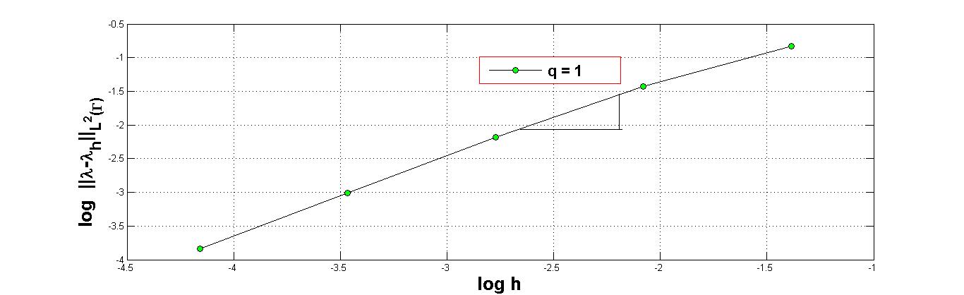 Figure 1
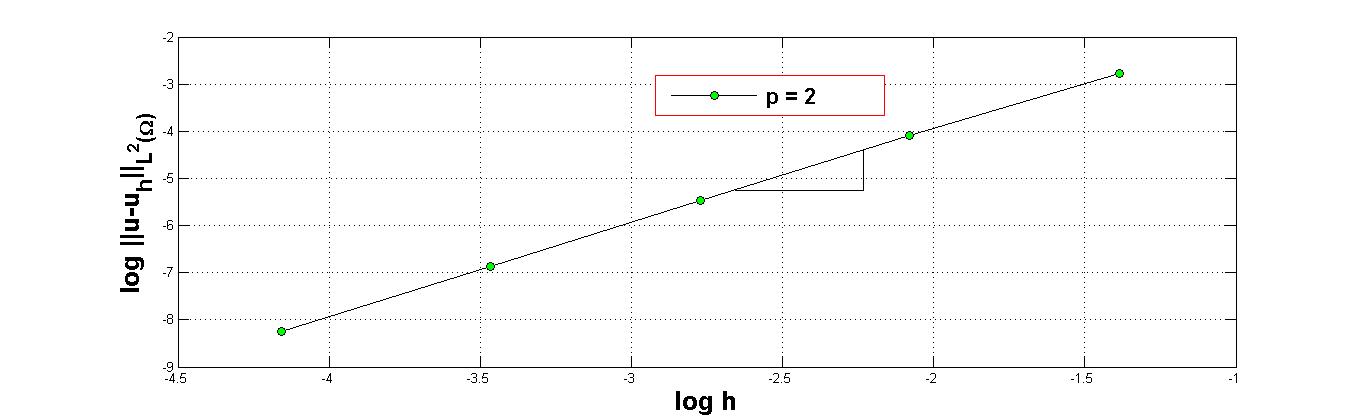 Figure 2
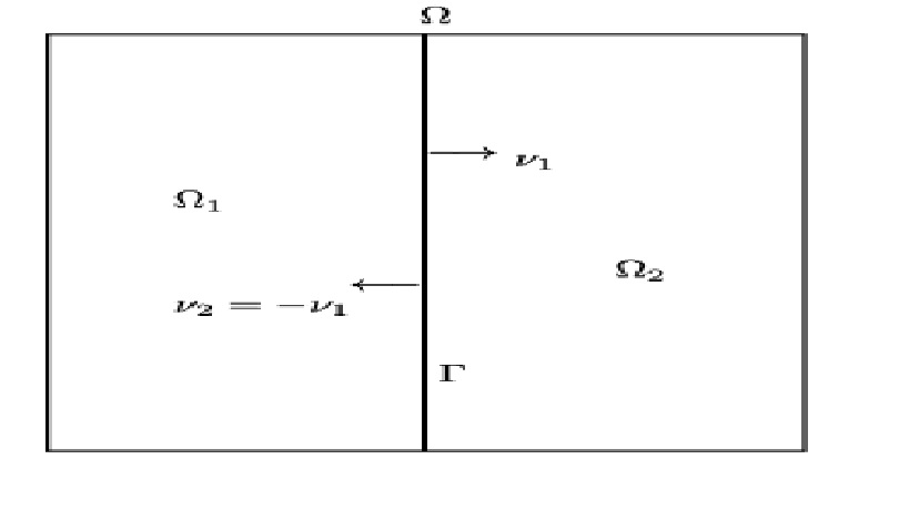 Figure 3
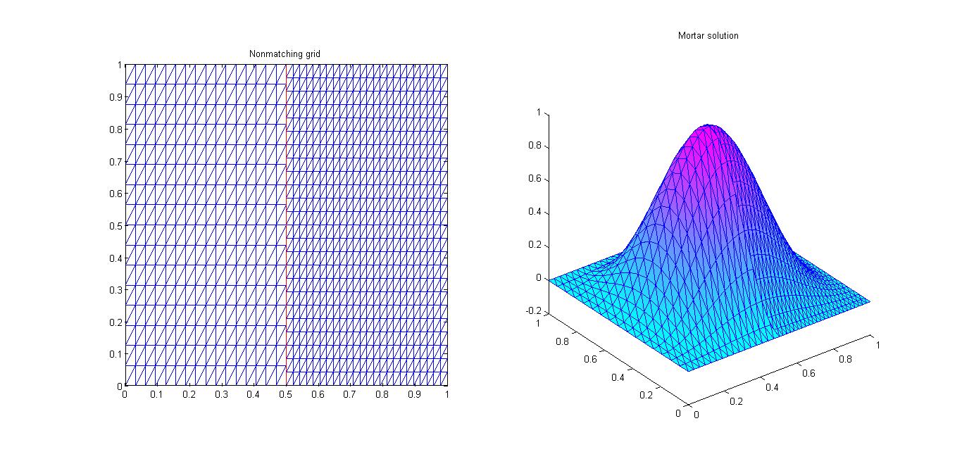 Figure 4
| 1/4 | 0.062158 | 0.43687 | |||
| 1/8 | 0.016638 | 0.24098 | 1.901458062028300 | 0.858290623104806 | |
| 1/16 | 0.0041882 | 0.11229 | 1.990079779863557 | 1.101683961685886 | |
| 1/32 | 0.0010422 | 0.049426 | 2.006698177352890 | 1.183887393718836 | |
| 1/64 | 0.00025934 | 0.021541 | 2.006715513479729 | 1.198184929427100 |
| 1/4 | 0.061619 | 0.45209 | |||
| 1/8 | 0.016431 | 0.25338 | 1.906954983214551 | 0.835307353359031 | |
| 1/16 | 0.0041218 | 0.11953 | 1.995073877668074 | 1.083929897366207 | |
| 1/32 | 0.0010233 | 0.052978 | 2.010045342634421 | 1.173907469688573 | |
| 1/64 | 0.00025429 | 0.023106 | 2.008682526770985 | 1.197125851836898 |
| 1/4 | 0.058294 | 1.8372e-07 | |||
| 1/8 | 0.015655 | 6.2439e-08 | 1.896723890974834 | 1.556989351729802 | |
| 1/16 | 0.0040013 | 2.366e-08 | 1.968082803651483 | 1.399997358151351 | |
| 1/32 | 0.0010066 | 1.032e-08 | 1.990978296765009 | 1.197007102916534 | |
| 1/64 | 0.00025206 | 5.325e-09 | 1.997651406176591 | 0.954589540310056 |
Peer Reviews
No public reviews on file for this paper yet. If you reviewed it on a platform where reviews are public (OpenReview, ICLR, NeurIPS, ICML), you can paste yours below so the community can read it here.
Videos
No videos yet. Explain this paper in a talk, walkthrough, or lecture? Add one.
Taxonomy
TopicsAdvanced Numerical Methods in Computational Mathematics · Numerical methods in engineering · Differential Equations and Numerical Methods
Convergence results with natural norms: Stabilized Lagrange multiplier method for elliptic interface problems
Sanjib Kumar Acharya
The LNM Institute of Information Technology, Jaipur 302031, Rajasthan, India
and
Ajit Patel
The LNM Institute of Information Technology, Jaipur 302031, Rajasthan, India
Abstract.
A stabilized Lagrange multiplier method for second order elliptic interface problems is presented in the framework of mortar method. The requirement of LBB (Ladyzhenskaya-Babuška-Brezzi) condition for mortar method is alleviated by introducing penalty terms in the formulation. Optimal convergence results are established in natural norm which is independent of mesh. Numerical experiments are conducted in support of the theoretical derivations.
2010 Mathematics Subject Classification:
65N30, 35J15, 35J25
1. Introduction
The best part of considering Lagrange multiplier formulation is: it converts a constraint problem in to an unconstrained problem which is comparably an easy way for implementation (see [1]). Also, we can evaluate both primal and flux variable simultaneously. On the other hand, one major difficulty in considering the Lagrange multiplier method is: the finite dimensional problems have to obey the inf-sup condition (LBB condition) which rejects many natural choices for approximation. Fortunately this requirement has been alleviated by Barbosa and Hughes (see [5]). They proposed a stabilized multiplier method which is stable and optimally convergent with respect to a mesh-dependent norm. In [6] the convergence results of these methods are established with natural norms. Nitsche had introduced a penalty term on the boundary to derive optimal estimates for approximating elliptic problems with nonhomogeneous Dirichlet boundary condition without enforcing boundary condition on the finite element spaces in [14].
These ideas are extended to multi-domain problems with non-matching grids by Hansbo et al. in [13] and Becker et al. in [7]. Wherein, the optimal convergence results are established in mesh-dependent norm. In [13], a stabilization method has been proposed, which uses global polynomials as multipliers to avoid the cumbersome integration of products of unrelated mesh functions and derived the stability under the condition that the approximation space for the interface multiplier contains the constant. A Lagrange multiplier method with penalty for multi-domain problems with non-matching grid is discussed by Patel (see [15]) which is well-posed and stable but due to inconsistency there is loss of accuracy. Stenberg has pointed out a close connection between Nitsche’s method and stabilized schemes and proposed it as mortaring Nitsche method (see [16]). For a detail study, we refer to [7, 8, 9, 13, 16].
In this paper, we extend the ideas of [6] to multi-domain problems with non-matching grid and establish the optimal error estimates in natural norm. Here, the multipliers are simply the nodal basis functions restricted to the interface. Error estimates are obtained with an assumption that: the multiplier space satisfies the strong regularity property in the sense of Babuška (see [1]). We give some computational results in support of the theoretical results.
A brief outline is as follows. We recall some functional spaces and approximation results in Section 2. In Section 3 we define the stabilized Lagrange multiplier methods for an elliptic interface problem and derive the error estimates. We give a matrix formulation of the method in Section 4. In Section 5, some numerical experiments are given. Finally, we concluded in Section 6.
2. Preliminaries
Let be an open bounded polygonal domain in with boundary . We define as a -tuple of non-negative integers and with set
[TABLE]
The Sobolev space of order (see [12]) over is defined as
[TABLE]
equipped with the norm and semi-norm
[TABLE]
respectively. Let be a positive real number, where and are the integral and fractional part of respectively. The fractional Sobolev space is defined as
[TABLE]
with the norm
[TABLE]
We shall denote by the space of traces over of the functions equipped with the norm
[TABLE]
and
[TABLE]
Let be the dual space of equipped with the norm
[TABLE]
where is the duality pairing between and . With , let be an extension of by zero to all of . Then we set , a subspace of as
[TABLE]
The norm in is defined by:
[TABLE]
Let be the dual space of . Also denote the duality pairing between and and let the norm on be defined by
[TABLE]
Note that, is continuously embedded into (see [9]).
Let and be the common interface (see Figure 1). We denote the unit outward normal oriented from towards and . For any function let . Let
[TABLE]
Now we define
[TABLE]
equipped with the norm
[TABLE]
and the multiplier space .
Let be a family of triangulation (in the sense of Ciarlet, see [10]) of with triangles or parallelograms. For let , , and . Suppose there exist positive constants and independent of such that for all verifies the quasiuniform condition and the shape regularity .
We define finite dimensional subspaces on each subdomain as
[TABLE]
We set and define the global space defined as
[TABLE]
Let be the restriction of to . Assume two different 1D triangulations on , and and correspondingly two different trace spaces and . For our convenience we may choose the multiplier space to be . Now we recall the following approximation results (see [10, 15]).
Lemma 2.1**.**
For all there exists a constant independent of such that
[TABLE]
We assume denotes a generic constant throughout the discussion.
Lemma 2.2**.**
Let for and . Then there exist constants independent of and a sequence such that for any
[TABLE]
For we set the interpolation as: equals on each for . We define the projection from onto as below:
for all ,
[TABLE]
Lemma 2.3**.**
[8*]**
For any , the following estimate holds: for all there exists a constant independent of such that*
[TABLE]
where .
3. Problem formulation and error estimates
Consider a second order elliptic interface model problem: for
[TABLE]
where is discontinuous along but piecewise smooth in each subdomain, is an appropriate smooth function, for some positive constants and and for all , . Also .
The mixed formulation of (3.1)-(3.3) is to seek a pair such that
[TABLE]
[TABLE]
[TABLE]
and is the Lagrange multiplier. We note that the bilinear forms and are continuous in and respectively.
The stabilized Nitsche’s mortaring approximation is: find such that
[TABLE]
where
[TABLE]
Here, and is penalty parameter to be chosen later. When the above formulation is unsymmetric and for , the formulation is symmetric.
Remark 3.1*.*
In the paper [13] a stabilized Lagrange multiplier formulation to circumvent the inf-sup condition has been introduced where they used global polynomials over the interfaces as multipliers to avoid cumbersome integrations of functions from two different non-matching sides. We also propose a similar formulation but here we take the trace space as multiplier space, which involves integration of non-matched functions. But our aim here is to derive the error estimates in natural norms. These estimates can be extended for the case: using global polynomials as multipliers as in [13].
For any it is easy to check that the problem (3.5) is consistent with the original problem (3.4) and hence the following lemma follows.
Lemma 3.2**.**
The problem (3.5) is consistent with the original problem (3.4). Moreover, if is the solution of (3.4) and is the solution of (3.5), then
[TABLE]
Lemma 3.3**.**
There exists independent of such that for all : \mathcal{A}(v_{h},\mu_{h};v_{h},-\mu_{h})\geq\alpha\bigg{(}\sum^{2}_{i=1}{||v_{h}||}^{2}_{H^{1}(\Omega_{i})}+{||\gamma^{1/2}\mu_{h}||}^{2}_{L^{2}(\Gamma)}\bigg{)} for with , is a positive constant.
Proof.
Taking and in (3.6), we arrive at
[TABLE]
Using Cauchy-Schwarz inequality, Young’s inequality, Lemma 2.1 and using the bounds for , we find the third term in the right hand side of (3.8) as
[TABLE]
Substituting (3.9) in (3.8) and using the bounds for and , we find
[TABLE]
Hence the result follows. ∎
Note that the uniqueness of the solution of (3.5) is evident from the coercivity property (Lemma 3.3) of which establish the existence of the solution.
Theorem 3.4**.**
Let and be the solutions of (3.4) and (3.5) respectively with . Further, assume satisfies the strong regular property in the sense of Babuška (see [1]): there exists a constant such that
[TABLE]
Then for , there exists a positive constant independent of and such that the errors and satisfies:
[TABLE]
Remark 3.5*.*
The space satisfying the strong regularity condition can be constructed using the technique of Hill functions, as in [2, 3] (see [1] page 186 for a discussion).
In order to prove the above theorem we require following results:
Lemma 3.6**.**
There exist positive constants and such that for all ,
[TABLE]
Proof.
For , let be the solution of the following mixed boundary value problem:
[TABLE]
Then there exist constants such that:
[TABLE]
Also from [1], we have
[TABLE]
Let be the Galerkin finite element approximation solution of (3.13), that is
[TABLE]
Summing over we find:
[TABLE]
and
[TABLE]
From (3.17), we arrive at
[TABLE]
Also, from triangle inequality, (3.14), (3.15) and (3.18), we find
[TABLE]
Hence, the Lemma follows from (3.19) and (3.20). ∎
Lemma 3.7**.**
If then there exists such that
[TABLE]
Proof.
Applying Cauchy-Schwarz inequality and duality between and , we arrive at
[TABLE]
Hence, (3.21) follows by using Lemma 2.1 and the hypothesis (3.10). In a similar way, we can derive (3.22). ∎
Lemma 3.8**.**
There exists a constant such that for :
[TABLE]
Proof.
Using (3.6), Lemma 3.7 and Young’s inequality, we find
[TABLE]
Now let be the function for which supremum occurs in condition (3.12) and assume that . Then using Lemma 2.1,
[TABLE]
Let . Considering and using the Lemma 3.3, we find
[TABLE]
Here, and are positive constants. Further,
[TABLE]
Hence, (3.23) follows from (3.26) and (3.27). ∎
Proof.
of Theorem 3.4: From Lemma 3.8, there exist a pair such that
[TABLE]
and that implies
[TABLE]
From (3.29) and orthogonality (3.7) of , we find
[TABLE]
[TABLE]
Note that
[TABLE]
Hence, from (3.28), (3.30), Lemma 2.2 and Lemma 2.3, the (3.11) follows. ∎
For the -error estimate, we appeal to the Aubin-Nitsche duality argument. Let be the solution of the interface problem
[TABLE]
which satisfies the regularity condition (see [4], [11])
[TABLE]
Theorem 3.9**.**
Let denotes the form with . Also let and be the solutions of respective equations as in Theorem 3.4 with . Then for , there exists a positive constant independent of and such that
[TABLE]
Proof.
Clearly satisfies , where is the Lagrange multiplier. By symmetric property and orthogonality,
[TABLE]
Using Cauchy-Schwarz inequality, the duality paring between and and trace inequality, we find
[TABLE]
Using trace inequality and Lemma 2.1, we find
[TABLE]
From (3.36) and (3.37) using Theorem 3.4, Lemma 2.2 and Lemma 2.3 with , we arrive at
[TABLE]
Hence, (3.35) follows by using the regularity condition (3.34). ∎
Remark 3.10*.*
For unsymmetric case, when , the -error estimate is of . However, with an additional assumption on the interpolants and i.e.,
[TABLE]
we can establish optimal order of -estimate in a similar way as in Barbosa et al. (see [6]).
4. Matrix formulation
The stabilized Nitsche’s mortaring method (3.5) can be represented in matrix form by .
The stiffness matrix
[TABLE]
where, for ,
[TABLE]
Also, U=\big{(}u^{1}_{i},u^{1}_{s},u^{2}_{i},u^{2}_{m},\lambda_{m}\big{)}^{T}. The unknowns and are associated with the internal nodes in and respectively. Unknown and are associated with and and are the unknown Lagrange multipliers associated with .
The load vector where,
[TABLE]
Here, are the nodal basis functions for , and are the basis functions for and respectively.
5. Numerical experiments
We choose problem (3.1)-(3.3) over the unit square domain . We divide the domain into two equal subdomains (see Figure 2). Each subdomains further subdivided into linear triangular elements of different mesh size . We choose the penalty parameter to be . Set and to be zero. We choose such that the exact solution of the problem is .
The order of convergence ‘’ for the error and the order of convergence ‘’ for the error with respect to the discretization parameter are computed by taking discontinuous coefficients pairs , , in the subdomains and , see Tables 1, 2, 3. Figure 3 (a) shows the computed order of convergence for with respect to in the log-log scale. Figure 3 (b) shows the convergence rate of the Lagrange multiplier with respect to . Note that, since the exact solution is smooth, the convergence rates of error and are computationally obtained as expected i.e., and respectively.
6. Conclusion
In order to alleviate the inf-sup condition in the mortar method with Lagrange multiplier, a stabilized method is presented and optimal error estimates are obtained in natural norm which is independent of mesh. Numerical experiments presented here depict the performance of the method and supports the theoretical error estimates. Here, the multipliers are simply the nodal basis functions restricted to the interface, one can consider global polynomials as multipliers as in [13] to avoid the cumbersome integration over unrelated meshes.
The reference list from the paper itself. Each links out to its DOI / PubMed record.
- 1[1] I. Babuška, The finite element method with Lagrange multipliers, Numer. Math. 16 (1973) pp. 179–192.
- 2[2] I. Babuška, Approximation by Hill functions, Commentations Math. Univ. Carolinae 11 (1970) pp. 387–811.
- 3[3] I. Babuška, Approximation by Hill functions II, Commentations Math. Univ. Carolinae 13 (1972) pp. 1–22.
- 4[4] I. Babuška, The finite element method for elliptic equations with discontinuous coefficients, Computing (Arch. Elektron. Rechnen) 5, (1970) pp. 207–213.
- 5[5] H. J. C. Barbosa and T. J. R. Hughes, The finite element method with Lagrange multipliers on the boundary: Circumventing the Babuška-Brezzi condition, Comput. Methods Appl. Mech. Eng. 85 (1991) pp. 109–128.
- 6[6] H. J. C. Barbosa and T. J. R. Hughes, Boundary Lagrange multipliers in the finite element methods: error analysis in natural norms, Numer. Math. 62 (1992) pp. 1–15.
- 7[7] R. Becker, P. Hansbo and R. Stenberg, A finite element method for domain decomposition with non-matching grids, M 2AN Math. Model. Numer. Anal. 37 (2003) pp. 209–225.
- 8[8] C. Bernardi, Y. Maday and A. T. Patera, A new nonconforming approach to domain decomposition: The mortar element method, In collége de France Seminar (1990).