This paper proves the asymptotic normality and consistency of the maximum likelihood estimator in complex Markov regime switching models, including those with zero transition probabilities and regime-dependent densities.
Contribution
It establishes the asymptotic properties of the MLE for a broad class of Markov regime switching models previously lacking such theoretical validation.
Findings
01
MLE is asymptotically normal in these models
02
Consistency of the covariance matrix estimator is proven
03
Applicable to models with zero transition probabilities and regime-dependent densities
Abstract
Markov regime switching models have been widely used in numerous empirical applications in economics and finance. However, the asymptotic distribution of the maximum likelihood estimator (MLE) has not been proven for some empirically popular Markov regime switching models. In particular, the asymptotic distribution of the MLE has been unknown for models in which some elements of the transition probability matrix have the value of zero, as is commonly assumed in empirical applications with models with more than two regimes. This also includes models in which the regime-specific density depends on both the current and the lagged regimes such as the seminal model of Hamilton (1989) and switching ARCH model of Hamilton and Susmel (1994). This paper shows the asymptotic normality of the MLE and consistency of the asymptotic covariance matrix estimate of these models.
Figures2
Click any figure to enlarge with its caption.
Figure 1
Figure 2
Tables3
Table 1. Table 1: Coverage probability of the asymptotic 95% confidence intervals for Hamilton’s model
Panel A: 95% confidence intervals constructed from (18)
0.916
0.911
0.938
0.926
0.944
0.925
0.916
0.896
0.875
0.938
0.933
0.930
0.944
0.943
0.937
0.946
0.929
0.922
0.942
0.942
0.945
0.941
0.950
0.956
0.939
0.941
0.930
Panel B: 95% confidence intervals constructed from the OPG estimator
0.915
0.920
0.938
0.927
0.941
0.934
0.922
0.901
0.884
0.932
0.932
0.938
0.949
0.942
0.939
0.945
0.929
0.923
0.943
0.945
0.945
0.939
0.949
0.956
0.936
0.937
0.929
Table 2. Table 2: Coverage probability of the asymptotic 95% confidence intervals for the MS-CD model
No public reviews on file for this paper yet. If you reviewed it on a platform where reviews are public (OpenReview, ICLR, NeurIPS, ICML), you can paste yours below so the community can read it here.
Videos
No videos yet. Explain this paper in a talk, walkthrough, or lecture? Add one.
Taxonomy
TopicsMonetary Policy and Economic Impact · Financial Risk and Volatility Modeling · Stochastic processes and financial applications
Full text
**Asymptotic Properties of the Maximum Likelihood Estimator
in Regime Switching Econometric Models††thanks: This research was supported by the Natural Science and Engineering Research Council of Canada and JSPS KAKENHI Grant Number JP17K03653.**
Markov regime switching models have been widely used in numerous empirical applications in economics and finance. However, the asymptotic distribution of the maximum likelihood estimator (MLE) has not been proven for some empirically popular Markov regime switching models. In particular, the asymptotic distribution of the MLE has been unknown for models in which some elements of the transition probability matrix have the value of zero, as is commonly assumed in empirical applications with models with more than two regimes. This also includes models in which the regime-specific density depends on both the current and the lagged regimes such as the seminal model of Hamilton (1989) and switching ARCH model of Hamilton and Susmel (1994). This paper shows the asymptotic normality of the MLE and consistency of the asymptotic covariance matrix estimate of these models.
Since the seminal contribution of Hamilton (1989), Markov regime switching models have become a popular framework for applied empirical work because they can capture the important features of time series such as structural changes, nonlinearity, high persistence, fat tails, leptokurtosis, and asymmetric dependence (e.g., Evans and Wachtel, 1993; Hamilton and Susmel, 1994; Gray, 1996; Sims and Zha, 2006; Inoue and Okimoto, 2008; Ang and Bekaert, 2002; Okimoto, 2008; Dai et al., 2007). Surveys of applications of Markov regime switching models in economics and finance are provided by, for example, Hamilton (2008, 2016) and Ang and Timmermann (2012).
Consider the Markov regime switching model defined by a discrete-time stochastic process {Yk,Xk} written as
[TABLE]
where {εk} is an independent and identically distributed sequence of random variables, {Yk} is an inhomogeneous s-order Markov chain on a state space Y conditional on Xk such that the conditional distribution of Yk only depends on Xk and the lagged Y’s, Xk is a first-order Markov process in a state space X, and fθ is a family of functions indexed by a finite-dimensional parameter θ∈Θ. In (1), the Markov chain {Xk} is not observable.
Surprisingly, the asymptotic distribution of the maximum likelihood estimator (MLE) of the Markov regime switching model (1) has not been fully established in the existing literature. Bickel et al. (1998) and Jensen and Petersen (1999) derive the asymptotic normality of the MLE of hidden Markov models in which the conditional distribution of Yk depends on Xk but not on the lagged Y’s. For hidden Markov models and Markov regime switching models with a finite state space, the consistency of the MLE has been proven by Leroux (1992), Francq and Roussignol (1998), and Krishnamurthy and Rydén (1998).
In an influential paper, Douc et al. (2004) [DMR hereafter] establish the consistency and asymptotic normality of the MLE in autoregressive Markov regime switching models (1) with a nonfinite hidden state space X under two assumptions. First, DMR assume that the conditional distribution of Yk does not depend on the lagged Xk’s. Specifically, on page 2259, DMR assume that
for each n≥1 and given {Yk}k=n−sn−1 and Xn, Yn is conditionally independent of {Yk}k=−s+1n−s−1
and {Xk}k=0n−1.
Second, DMR assume in their Assumption A1(a) that the transition density of Xk is bounded away from 0.
These two assumptions together rule out regime switching models in which some elements of the transition probability matrix take the value of zero. However, empirical researchers often assume that some elements of the transition probability matrix are identically equal to zero when they estimate regime switching models with more than two regimes. For example, Kim et al. (2005) estimate a three-regime model of U.S. GDP growth in which some elements of the transition probability matrix are restricted to be zero because “the three regimes corresponding to expansion, recession and recovery always occur in that order” (see also Boldin (1996)). Similarly, Dahlquista and Gray (2000) estimate a three-regime model of short-term interest rates for France and Italy while restricting some elements of the transition probability matrix to be zero and David and Veronesi (2013) estimate a six-regime model of inflation, earnings growth, consumption growth, S&P 500 P/E ratios, the three-month Treasury bill rate, and one- and five-year Treasury bond yields in which the transition probability matrix is parameterized with five parameters with some elements restricted to zero. Assumption A1(a) of DMR does not hold in these papers.
The two assumptions imposed by DMR also rule out models in which the conditional density Yk depends on both the current and the lagged regimes. Suppose that we specify Xk in (1) as
[TABLE]
where p≥2, and Xk follows a first-order Markov process and is called the regime. Then, the transition density of Xk inevitably has zeros. For example, when p=2 and Xk=(X~k,X~k−1), we have Pr(Xk+1=(i′,j′)∣Xk=(i,j))=0 when j′=i. Consequently, the asymptotic distribution of the MLE has not been proven for some popular Markov regime switching models including the seminal model of Hamilton (1989) and switching ARCH (SWARCH) model of Hamilton and Susmel (1994).
where εk∼ i.i.d. N(0,1) and X~k follows a Markov chain on X~={1,2,…,M} with Pr(X~k=j∣X~k−1=i)=pij, where M represents the number of regimes.
Hamilton (1989) estimates model (3) with M=2 and p=5 by using data on U.S. real GNP growth.
McConnel and Perez-Quiros (2000) and Camacho and Perez-Quiros (2007) estimate an augmented model (3) that allows the standard deviation parameter σ in (3) to be regime-dependent.
Example 2** (SWARCH model of Hamilton and Susmel (1994)).**
Consider the following model:
[TABLE]
*where εk∼ i.i.d. N(0,1) or Student t with v degrees of freedom, and X~k follows a Markov chain on X~={1,2,…,M} with Pr(X~k=j∣X~k−1=i)=pij.
*
Example 3** (Bounce-back effect model of Kim et al. (2005)).**
Consider the following model:
[TABLE]
where X~k follows a Markov chain on X~={1,2,…,M} with Pr(X~k=j∣X~k−1=i)=pij. Kim et al. (2005) use this model with p=6 to capture the post-recession “bounce-back” effect in U.S. quarterly GDP.
In examples 1–3, the transition probability of Xk=(X~k,…,X~k−p+1)′ has zeros when p≥2. Therefore, Assumption A1(a) of DMR is violated. As discussed on pages 2257–2258 of DMR, Assumption A1(a) is crucial for their Corollary 1 (page 2262) that establishes the deterministic geometrically decaying bound on the mixing rate of the conditional chain, X∣Y. As DMR recognize on page 2258, this deterministic nature of the bound is vital to their proof of the asymptotic normality of the MLE.
This paper shows the consistency and asymptotic normality of the MLE of the Markov regime switching model in which some elements of the transition probability matrix of Xk are zero. To the best of our knowledge, there exists no rigorous proof in the literature of the asymptotic normality of the MLE of these regime switching models, even though empirical researchers often assume that some elements of the transition probability matrix are zero and the models of Hamilton (1989) and Hamilton and Susmel (1994) are popular in applied work. This is an important gap in the literature to be filled because empirical researchers regularly make inferences based on the presumed asymptotic normality (e.g., Goodwin, 1993; Garcia and Perron, 1996; Hamilton and Lin, 1996; Fong, 1997; Ramchand and Susmel, 1998; Maheu and McCurdy, 2000; McConnel and Perez-Quiros, 2000; Edwards and Susmel, 2001; Camacho and Perez-Quiros, 2007). This paper therefore provides the theoretical basis for the statistical inferences associated with these models.
To derive the asymptotic normality of the MLE, we first establish a bound on the mixing rate of the conditional chain, X∣Y, in Lemma 1. Our bound is written as a product of random variables, where all but finitely many of them are strictly less than 1. Consequently, the mixing rate of the conditional chain is geometrically decaying almost surely. We then use this mixing rate to show that the sequence of the conditional scores and conditional Hessians given the m past periods converge to the conditional score and conditional Hessian given the “infinite past” as m→∞. Given these results, we show the asymptotic normality of the MLE under standard regularity assumptions by applying a martingale central limit theorem to the score function (Proposition 2) as well as by proving a uniform law of large numbers for the observed Fisher information (Proposition 3). These results extend those in DMR to an empirically important class of models where the transition density has the value of zero. Another feature of the present study is that we introduce an additional weakly exogenous regressor, Wk.
We also relax the assumption in DMR on the regime-specific density. DMR assume that the regime-specific density is uniformly bounded with respect to Xk and θ, whereas we only assume the existence of the first moment of the supremum of the logarithm of the regime-specific density with respect to Xk and θ. Unbounded densities are used in other analyses (e.g., Zinde-Walsh, 2008) and empirical studies.
Example 4** (Markov regime-switching conditional duration (MS-CD) model).**
Consider the following model:
[TABLE]
where εk follows the standardized Weibull distribution with E(εk)=1, μXk is a regime-dependent parameter, and Xk∈{1,2,…,M} is a regime in period k. The density of Yk conditional on Yk−1 and Xk is given by gθ(yk∣Yk−1,Xk)=λk(Yk−1,Xk)γ(λk(Yk−1,Xk)yk)γ−1exp{−(λk(Yk−1,Xk)yk)γ}, where λk(Yk−1,Xk)=Γ(1+1/γ)μXk+βYk−1. In this model, the regime-specific density is unbounded when γ<1.
Our simulations based on the model (4) show that the asymptotic distribution provides a good approximation of the finite sample behavior of the MLE even when the regime-specific density is unbounded.
In regime switching models, testing for the number of regimes (number of elements in X) has been an unsolved problem because the standard asymptotic analysis of the likelihood ratio test statistic (LRTS) breaks down. In testing the null hypothesis of no regime switching, the asymptotic behavior of the LRTS has been investigated by Hansen (1992) and Garcia (1998); Carrasco et al. (2014) propose an information matrix-type test and Cho and White (2007) derive the asymptotic distribution of the quasi-LRTS. Recently, Qu and Zhuo (2017) derive the asymptotic distribution of the LRTS of testing the null hypothesis of no regime switching under some restrictions on the transition probabilities of regimes and Rabah (2012) compares the finite sample performance of the bootstrapped LRTS with the test of Carrasco et al. (2014). Kasahara and Shimotsu (2018) derive the asymptotic distribution of the LRTS for testing the null hypothesis of M regimes against the alternative hypothesis of M+1 regimes for any M≥1 and show the asymptotic validity of the parametric bootstrap.
The remainder of this paper is organized as follows. Section 2 introduces the notation, model, and assumptions. Section 3 derives the bound on the mixing rate of the conditional chain, X∣Y. Section 4 derives the consistency of the MLE, and the asymptotic normality of the MLE is shown in Section 5. Section 6 reports the simulation results. Appendix A collects the proofs and Appendix B collects the auxiliary results.
2 Model and assumptions
Our notation largely follows the notation in DMR. Let := denote “equals by definition.” For a k×1 vector x=(x1,…,xk)′ and a matrix B, define ∣x∣:=x′x and ∣B∣:=λmax(B′B), where λmax(B′B) denotes the largest eigenvalue of B′B. For a k×1 vector a=(a1,…,ak)′ and a function f(a), let ∇a2f(a):=∇aa′f(a). For two probability measures μ1 and μ2, the total variation distance between μ1 and μ2 is defined as ∥μ1−μ2∥TV:=supA∣μ1(A)−μ2(A)∣. ∥⋅∥TV satisfies supf(x):0≤f(x)≤1∣∫f(x)μ1(dx)−∫f(x)μ2(dx)∣=∥μ1−μ2∥TV and supf(x):maxx∣f(x)∣≤1∣∫f(x)μ1(dx)−∫f(x)μ2(dx)∣=2∥μ1−μ2∥TV for any two probability measures μ1 and μ2 (e.g., Levin et al. (2009, Proposition 4.5)). Let I{A} denote an indicator function that takes the value of one when A is true and zero otherwise. For a metric space A, let Ak denote the k-fold product space of A. C denotes a generic finite positive constant whose value may change from one expression to another. Let a∨b:=max{a,b} and a∧b:=min{a,b}. Let ⌊x⌋ denote the largest integer less than or equal to x, and define (x)+:=max{x,0}. For any {xi}, we define ∑i=abxi:=0 and ∏i=abxi:=1 when b<a. “i.o.” stands for “infinitely often.” All the limits below are taken as n→∞ unless stated otherwise.
We consider the Markov regime switching process defined by a discrete-time stochastic process {(Xk,Yk,Wk)}, where (Xk,Yk,Wk) takes the values in a set X×Y×W with the associated Borel σ-field B(X×Y×W). We use pθ(⋅) to denote densities with respect to the probability measure on B(X×Y×W)⊗Z. For a stochastic process {Uk} and a<b, define Uab:=(Ua,Ua+1,…,Ub). Denote Yk−1:=(Yk−1,…,Yk−s) for a fixed integer s and Yab:=(Ya,Ya+1,…,Yb). Define Zk:=(Xk,Yk). Let Qθ(x,A):=Pθ(Xk∈A∣Xk−1=x) denote the transition kernel of {Xk}k=0∞. Let Qθr(x,A):=Pθ(Xk∈A∣Xk−r=x) denote the r-step transition kernel of {Xk}k=0∞.
We now introduce our assumptions, which mainly follow the assumptions in DMR.
Assumption 1**.**
(a) The parameter θ belongs to Θ, a compact subset of Rq, and the true parameter value θ∗ lies in the interior of Θ. (b) {Xk}k=0∞ is a Markov chain that lies in a compact set X⊂Rdx. (c) For all θ∈Θ, Qθ(x,⋅) and Qθr(x,⋅) have densities qθ(x,⋅) and qθr(x,⋅), respectively, with respect to a finite dominating measure μ on B(X) such that μ(X)=1, and σ+0:=supθ∈Θsupx,x′∈Xqθ(x,x′)<∞. (d) There exists a finite p≥1 such that 0<σ−:=infθ∈Θinfxk−p,xk∈Xqθp(xk−p,xk) and σ+:=supθ∈Θsupxk−p,xk∈Xqθp(xk−p,xk)<∞. (e) {(Yk,Wk)}k=−s+1∞ takes the values in a set Y×W⊂Rdy×Rdw.
Assumption 2**.**
(a) For each k≥1, Xk is conditionally independent of (X0k−2,Y0k−1,W0∞) given Xk−1. (b) For each k≥1, Yk is conditionally independent of (Y−s+1k−s−1,X0k−1,W0k−1,Wk+1∞) given (Yk−1,Xk,Wk), and the model of the conditional distribution of Yk has a density gθ(yk∣Yk−1,Xk,Wk) with respect to a σ-finite measure ν on B(Y). (c) W1∞ is conditionally independent of (Y0,X0) given W0. (d) {(Zk,Wk)}k=0∞ is a strictly stationary ergodic process.
Assumption 3**.**
For all y′∈Y, y∈Ys, and w∈W, 0<infθ∈Θinfx∈Xgθ(y′∣y,x,w) and supθ∈Θsupx∈Xgθ(y′∣y,x,w)<∞.
Assumption 1(c) is also assumed on page 2258 of DMR. This assumption excludes the case where X=R and μ is the Lebesgue measure but allows for continuously distributed Xk with finite support. If multiple p’s satisfy Assumption 1(d), we define p as the minimum of such p’s. Assumption 1(d) implies that the state space X of the Markov chain {Xk} is νp-small for some nontrivial measure νp on B(X). Therefore, for all θ∈Θ, the chain {Xk} is aperiodic and has a unique invariant distribution and is uniformly ergodic (Meyn and Tweedie, 2009, Theorem 16.0.2). Assumptions 2(a)(b) imply that Zk is conditionally independent of (Z0k−2,W0k−1,Wk+1∞) given (Zk−1,Wk); hence, {Zk}k=0∞ is a Markov chain on Z:=X×Ys given {Wk}k=0∞. Under Assumptions 2(a)–(c), the conditional density of Z0n given W0n is written as pθ(Z0n∣W0n)=pθ(Z0∣W0)∏k=1npθ(Zk∣Zk−1,Wk). Because {(Zk,Wk)}k=0∞ is stationary, we extend {(Zk,Wk)}k=0∞ to a stationary process {(Zk,Wk)}k=−∞∞ with doubly infinite time. We denote the probability and associated expectation of {(Zk,Wk)}k=∞∞ under stationarity by Pθ and Eθ, respectively.111DMR use Pθ and Eθ to denote the probability and expectation under stationarity because their Section 7 deals with the case when Z0 is drawn from an arbitrary distribution. Because we assume {(Zk,Wk)}k=∞∞ is stationary throughout this paper, we use notations such as Pθ and Eθ without an overline for simplicity. Assumption 3 is stronger than Assumption A1(b) in DMR, which assumes only 0<infθ∈Θ∫x∈Xgθ(y′∣y,x)μ(dx) and supθ∈Θ∫x∈Xgθ(y′∣y,x)μ(dx)<∞. When X is finite, Assumption 3 becomes identical to Assumption A3 of Francq and Roussignol (1998), who prove the consistency of the MLE when X is finite. It appears that assuming a lower bound on gθ similar to Assumption 3 is necessary to derive the asymptotics of the MLE when infθinfx,x′qθ(x,x′)=0. When p=1, we could weaken Assumption 3 to Assumption A1(b) in DMR, but we retain Assumption 3 to simplify the exposition and proof.
DMR assume p=1 in Assumption 1(d), meaning that the transition density qθ(x,x′) of the state variable Xk is uniformly bounded from below. DMR show that this lower bound on qθ(x,x′) translates into a deterministic lower bound on the conditional transition density of Xk given the observations of {(Yk,Wk)}k=0n. Owing to this deterministic lower bound, the chain {Xk} given {(Yk,Wk)}k=0n is geometrically mixing, and, consequently, the derivatives of the log-densities are also geometrically mixing and follow the law of large numbers and central limit theorem.
When p≥2, this lower bound is no longer deterministic and depends on the Yk’s. For example, suppose that X={−1,0,1}, which correspond to “recession,” “normal,” and “expansion” periods, respectively, P(Xk=1∣Xk−1=−1)=0, and Yk∣(Xk,Yk−1)∼N(0.6Yk−1+Xk,1). Then, observing a negative value of Yk−1 implies that the likely value of Xk−1 is −1, which in turn implies that the event {Xk=1} is unlikely. As Yk−1 approaches negative infinity, P(Xk=1∣Yk,Yk−1) approaches zero and no lower bound on the transition density of Xk−1 exists given (Yk,Yk−1).
We overcome the zero lower bound on qθ(x,x′) by noting that, in many econometric models, only extreme values of Yk−1 provide a strong signal on the value of Xk−1. Because Yk−1 takes such extreme values with a small probability, the transition probability of the chain {Xk} given {(Yk,Wk)}k=0n is bounded from below by a stochastic lower bound whose value is close to zero only with a small probability. As a result, the chain {Xk} given {(Yk,Wk)}k=0n is geometrically mixing with a probability close to one.
Following DMR, we analyze the conditional log-likelihood function given Y0, W0n, and X0=x0 rather than the stationary log-likelihood function given Y0 and W0n because, as explained in DMR (pages 2263–2264), the conditional initial density pθ(X0∣Y0k−1) cannot be easily computed in practice. The conditional density function of Y1n is
[TABLE]
where pθ(yk,xk∣yk−1,xk−1,wk)=qθ(xk−1,xk)gθ(yk∣yk−1,xk,wk). Assumptions 2(a)–(c) imply that for k≥1, Wk is conditionally independent of Z0k−1 given W0k−1 because p(Wk∣Z0k−1,W0k−1)=p(W0k,Z0k−1)/p(W0k−1,Z0k−1) and for j=k,k−1, p(W0j,Z0k−1)=p(Z0,W0j)∏t=1k−1p(Zt∣Zt−1,Wt)=p(W1j∣W0)p(Z0∣W0)∏t=1k−1p(Zt∣Zt−1,Wt). Therefore, for 1≤k≤n, we have
[TABLE]
In view of (6) and (7), we can write the conditional and stationary log-likelihood functions as
[TABLE]
Many applications use the log-likelihood function in which the conditional density pθ(Y1n∣Y0,W0n,x0) is integrated with respect to x0 over a probability measure ξ on B(X), where ξ can be fixed or treated as an additional parameter. We also analyze the resulting objective function:
[TABLE]
3 Uniform forgetting of the conditional hidden Markov chain
In this section, we establish a mixing rate of the conditional hidden Markov chain, which is the chain {Xk}k=−mn given (Y−mn,W−mn). The bounds on this mixing rate are instrumental in deriving the asymptotic properties of the MLE. The following lemma bounds the distance between the distributions of Xk given (Y−mn,W−mn) when starting from two different initial distributions μ1(⋅) and μ2(⋅) of X−m. In other words, this lemma provides the rate at which the conditional hidden Markov chain forgets its past. This lemma generalizes Corollary 1 of DMR, which shows that the conditional hidden Markov chain forgets its past at a deterministic exponential rate when p=1. As DMR note on page 2258, their deterministic rate holds only when p=1.
Lemma 1**.**
Assume Assumptions 1–3. Let m,n∈Z with −m≤n and θ∈Θ. Then, for all −m≤k≤n, all probability measures μ1 and μ2 on B(X), and all (y−mn,w−mn),
[TABLE]
where ω(yk−pk−1,wk−pk−1):=σ−/σ+ when p=1, and, when p≥2,222Strictly speaking, wk−p in ω(yk−pk−1,wk−pk−1) is superfluous because ω(yk−pk−1,wk−pk−1) does not depend on wk−p. We retain wk−p for notational simplicity.
[TABLE]
The convergence rate of the conditional hidden Markov chain depends on the minorization coefficient ω(Yk−pk−1,Wk−pk−1). If this coefficient is bounded away from 0, the chain forgets its past exponentially fast. When p≥2, this coefficient is not necessarily bounded away from 0 because infyk−pk−1,wk−pk−1ω(yk−pk−1,wk−pk−1) can be possibly 0. However, ω(Yk−pk−1,Wk−pk−1) becomes close to zero only when Yk−p+1k−1 takes an unlikely value because the denominator of ω(Yk−pk−1,Wk−pk−1) is finite and the numerator of ω(Yk−pk−1,Wk−pk−1) is a product of the conditional density gθ(y∣y,x,w). As a result, ω(Yk−pk−1,Wk−pk−1) is bounded away from 0 with a probability close to 1. In the following sections, we use this fact to establish the consistency and asymptotic normality of the MLE.
4 Consistency of the MLE
Define the conditional MLE of θ∗ given Y0, W0n, and X0=x0 as
[TABLE]
with ln(θ,x0) defined in (8). In this section, we prove the consistency of the conditional MLE. We introduce additional assumptions required for proving consistency.
Assumption 4**.**
*(a) Eθ∗∣logb+(Y01,W1)∣<∞, where
b+(Yk−1k,Wk):=supθ∈Θsupxk∈Xgθ(Yk∣Yk−1,xk,Wk). (b) Eθ∗∣logb−(Y01,W1)∣<∞, where
There exist constants α>0, C1,C2∈(0,∞), and β>1 such that, for any r>0,
[TABLE]
Assumption 4(a) relaxes Assumption (A3) of DMR, who assume that
supθ∈Θsupy1,y0,x,wgθ(y1∣y0,x,w)<∞ and hence the density is uniformly bounded. Assumption 4(b) is stronger than Assumption (A3) of DMR, who assume Eθ∗∣log(infθ∈Θ∫gθ(Y1∣Y0,x)μ(dx)∣<∞. Assumption 4 implies that Eθ∗supθ∈Θsupx∈X∣log(gθ(Y1∣Y0,x,W1))∣<∞, which is similar to the moment condition used in the standard maximum likelihood estimation, but the infimum is taken over x in addition to θ. Assumption 5 restricts the probability that
supθ∈Θsupxk∈Xgθ(Yk∣Yk−1,xk,Wk)/infθ∈Θinfxk∈Xgθ(Yk∣Yk−1,xk,Wk) takes an extremely large value. Assumption 5 is not restrictive because the right hand side of the inequality inside Pθ∗(⋅) is exponential in r and the bound C2r−β is a polynomial in r. An easily verifiable sufficient condition for Assumption 5 is Eθ∗∣log(b+(Y01,W1)/b−(Y01,W1))∣1+δ<∞ for some δ>0. This is because Pθ∗(b+(Y01,W1)/b−(Y01,W1)≥eαr)=Pθ∗(log(b+(Y01,W1)/b−(Y01,W1))≥αr)
≤(Eθ∗∣log(b+(Y01,W1)/b−(Y01,W1))∣1+δ)/(αr)1+δ≤C2r−(1+δ), where the first inequality follows from Markov’s inequality. Examples 1–4 satisfy Assumptions 4 and 5.
In the following lemma, we show that the difference between the conditional log-likelihood function ln(θ,x0) and the stationary log-likelihood function ln(θ) is o(n)Pθ∗-a.s.
When p=1, Lemma 2 of DMR shows that supθ∈Θ∣ln(θ,x0)−ln(θ)∣ is bounded by a deterministic constant. When p≥2, Lemma 2 of DMR is no longer applicable because ∣ln(θ,x0)−ln(θ)∣ depends on the products of 1−ω(Ypi−ppi−1,Wpi−ppi−1)’s for i=1,…,⌊n/p⌋. A key observation is that {ω(Ypi−ppi−1,Wpi−ppi−1)}i≥1 is stationary and ergodic and that ϵ:=Pθ∗(ω(Ypi−ppi−1,Wpi−ppi−1)≤δ) is small when δ>0 is sufficiently small. Because the strong law of large numbers implies that (⌊n/p⌋)−1∑i=1⌊n/p⌋I{ω(Ypi−ppi−1,Wpi−ppi−1)>δ} converges to 1−ϵPθ∗-a.s., 1−ω(Ypi−ppi−1,Wpi−ppi−1)≤1−δ holds for a large fraction of the ω(Ypi−ppi−1,Wpi−ppi−1)’s. Consequently, we can establish a Pθ∗-a.s. bound on n−1∣ln(θ,x0)−ln(θ)∣.
We proceed to show that, for all θ∈Θ, pθ(Yk∣Y−mk−1,W−mk) converges to pθ(Yk∣Y−∞k−1,W−∞k)Pθ∗-a.s. as m→∞ and that we can approximate n−1ln(θ) by n−1∑k=1nlogpθ(Yk∣Y−∞k−1,W−∞k), which is the sample average of the stationary ergodic random variables. For x∈X and m≥0, define
[TABLE]
so that ln(θ)=∑k=1nΔk,0(θ). The following proposition corresponds to Lemma 3 of DMR. This proposition shows that, for any k≥0, the sequences {Δk,m(θ)}m≥0 and {Δk,m,x(θ)}m≥0 are Cauchy uniformly in θ∈Θ.
Lemma 3**.**
Assume Assumptions 1–5. Then, there exist a constant ρ∈(0,1) and random sequences {Ak,m}k≥1,m≥0 and {Bk}k≥1 such that, for all 1≤k≤n and m′≥m≥0,
[TABLE]
where Pθ∗(Ak,m≥Mi.o.)=0 for a constant M<∞ and Bk∈L1(Pθ∗).
Lemma 3(a) implies that {Δk,m,x(θ)}m≥0 is a uniform Cauchy sequence in θ∈Θ with probability one and that limm→∞Δk,m,x(θ) does not depend on x. Let Δk,∞(θ) denote this limit. Because {Δk,m,x(θ)}m≥0 is uniformly bounded in L1(Pθ∗) from Lemma 3(c), {Δk,m,x(θ)}m≥0 converges to Δk,∞(θ) in L1(Pθ∗) and Δk,∞(θ)∈L1(Pθ∗) by the dominated convergence theorem. Define l(θ):=Eθ∗[Δ0,∞(θ)]. Lemma 3 also implies that n−1ln(θ) converge to n−1∑k=1nΔk,∞(θ), which converges to l(θ) by the ergodic theorem. Therefore, the consistency of θ^x0 is proven if this convergence of n−1ln(θ)−l(θ) is strengthened to uniform convergence in θ∈Θ and the additional regularity conditions are confirmed.
We introduce additional assumptions on the continuity of qθ and gθ and identification of θ∗.
Assumption 6**.**
(a) For all (y,y′,w)∈Ys×Y×W and uniformly in x,x′∈X, qθ(x,x′) and gθ(y′∣y,x,w) are continuous in θ. (b) Pθ∗[pθ∗(Y1∣Y−m0,W−m1)=pθ(Y1∣Y−m0,W−m1)]>0 for all m≥0 and all θ∈Θ such that θ=θ∗.
Assumption 6(b) is a high-level assumption because it is imposed on pθ(Y1∣Y−m0,W−m1). When the covariate Wk is absent, DMR prove consistency under a lower-level assumption (their (A5*′*)), which is stated in terms of pθ(Y1n∣Y0). We use Assumption 6(b) for brevity.
The following proposition shows the strong consistency of the (conditional) MLE.
Francq and Roussignol (1998, Theorem 3) prove the consistency of the MLE when the state space of Xk is finite. Proposition 1 generalizes Theorem 3 of Francq and Roussignol (1998) in the following three aspects. First, we allow Xk to be continuously distributed. Second, we analyze the log-likelihood function conditional on X0=x0, whereas Francq and Roussignol (1998) set the initial distribution of X1 to any probability vector with strictly positive elements. In other words, we allow for zeros in the postulated initial distribution of {Xk}. Third, we allow for an exogenous covariate {Wk}k=0n. Leroux (1992), Le Gland and Mevel (2000), and Douc and Matias (2001) analyze the asymptotic property of the MLE of hidden Markov models, which are the special case of the model considered here in that gθ(Yk∣Yk−1,Xk,Wk) does not depend on Yk−1.
Define the MLE with a probability measure ξ on B(X) for x0 as θ^ξ:=argmaxθ∈Θln(θ,ξ) with ln(θ,ξ) defined in (9). Proposition 1 implies the following corollary.
Corollary 1**.**
Assume Assumptions 1–6. Then, for any ξ, θ^ξ→θ∗Pθ∗-a.s.
5 Asymptotic distribution of the MLE
In this section, we derive the asymptotic distribution of the MLE and consistency of the asymptotic covariance matrix estimate. Because θ^x0 is consistent, expanding the first-order condition ∇θln(θ^x0,x0)=0 around θ∗ gives
[TABLE]
where θ∈[θ∗,θ^x0] and θ may take different values across different rows of ∇θ2ln(θ,x0). In the following, we approximate ∇θjln(θ,x0)=∑k=1n∇θjlogpθ(Yk∣Y0k−1,W0k,X0=x0) for j=1,2 by ∑k=1n∇θjlogpθ(Yk∣Y−∞k−1,W−∞k), which is a sum of a stationary process. We then apply the central limit theorem and law of large numbers to n−j/2∑k=1n∇θjlogpθ(Yk∣Y−∞k−1,W−∞k). A similar expansion gives the asymptotic distribution of n1/2(θ^ξ−θ∗).
We introduce additional assumptions. Define Xθ+:={(x,x′)∈X2:qθ(x,x′)>0}.
Assumption 7**.**
There exists a constant δ>0 such that the following conditions hold on G:={θ∈Θ:∣θ−θ∗∣<δ}: (a) For all (y,y′,w,x,x′)∈Ys×Y×W×X×X, the functions gθ(y′∣y,w,x) and qθ(x,x′) are twice continuously differentiable in θ∈G. (b) supθ∈Gsupx,x′∈Xθ+∣∇θlogqθ(x,x′)∣<∞ and supθ∈Gsupx,x′∈Xθ+∣∇θ2logqθ(x,x′)∣<∞. (c) Eθ∗[supθ∈Gsupx∈X∣∇θloggθ(Y1∣Y0,x,W1)∣2]<∞ and Eθ∗[supθ∈Gsupx∈X∣∇θ2loggθ(Y1∣Y0,x,W1)∣]<∞. (d) For almost all (y,y′,w)∈Ys×Y×W, there exists a function fy,y′,w:X→R+ in L1(μ) such that supθ∈Ggθ(y′∣y,x,w)≤fy,y′,w(x). (e) For almost all (x,y,w)∈X×Ys×W and j=1,2, there exist functions fx,y,wj:Y→R+ in L1(ν) such that ∣∇θjgθ(y′∣y,x,w)∣≤fx,y,wj(y′) for all θ∈G.
Assumption 7 is the same as Assumptions (A6)–(A8) of DMR except for accommodating the case inf(x,x′)∈X2qθ(x,x′)=0 and the covariate W. In Assumption 7(b), the supremum is taken over Xθ+ because ∇θlogqθ(x,x′) and ∇θ2logqθ(x,x′) are not well-defined when qθ(x,x′)=0. Examples 1–4 satisfy Assumption 7. Assumption 8 is a high-level assumption that bounds the moments of ∇θjlogpθ(Yk∣Y−mk−1,W−mk) and ∇θjlogpθ(Yk∣Y−mk−1,W−mk,X−m=x) uniformly in m. When p=1, DMR could derive Assumption 8 by using the L3−j(Pθ∗) convergence of ∇θjlogpθ(Yk∣Y−mk−1,W−mk) and ∇θjlogpθ(Yk∣Y−mk−1,W−mk,X−m=x) to ∇θjlogpθ(Yk∣Y−∞k−1,W−∞k) as m→∞. When p≥2, we need to assume Assumption 8 because our Lemma 4 only shows that these sequences converge to ∇θjlogpθ(Yk∣Y−∞k−1,W−∞k) in probability.
5.1 Asymptotic distribution of the score function
This section derives the asymptotic distribution of n−1/2∇θln(θ∗,x0) and n−1/2∇θln(θ∗,ξ). We introduce a result known as the Louis missing information principle (Louis, 1982), which expresses the derivatives of the log-likelihood function of a latent variable model in terms of the conditional expectation of the derivatives of the complete data log-likelihood function. Let (X,Y,W) be random variables with pθ(y,x∣w) denoting the joint density of (Y,X) given W, and let pθ(y∣w) be the marginal density of Y given W. Then, a straightforward differentiation that is valid under Assumption 7 gives ∇θlogpθ(Y∣W)=Eθ[∇θlogpθ(Y,X∣W)∣Y,W].
In terms of the variables in our model, we have, for any k≥1 and m≥0,
[TABLE]
where the last equality follows from Assumption 2.
Define Zk−1k:=(Yk,Xk,Yk−1,Xk−1). For j=1,2, denote the derivatives of the complete data log-density of (Yk,Xk) given (Yk−1,Xk−1,Wk) by
[TABLE]
We use a short-handed notation ϕθkj:=ϕj(θ,Zk−1k,Wk). We also suppress the superscript 1 from ϕθk1, so that ϕθk=ϕθk1. Let ∣ϕkj∣∞:=supθ∈Gsupx,x′∈Xθ+∣∇θjlogqθ(x,x′)∣+supθ∈Gsupx∈X∣∇θjloggθ(Yk∣Yk−1,x,Wk)∣.
Define, for x∈X, k≥1, m≥0, and j=1,2,333DMR (page 2272) use the symbol Δk,m,x(θ) to denote our Ψk,m,x1(θ), but we use Ψk,m,x(θ) to avoid confusion with Δk,m,x(θ) used in Lemma 3.
[TABLE]
It follows from (12) and (13) that Ψk,m,x1(θ)=∇θlogpθ(Y−m+1k∣Y−m,W−mk,X−m=x)−
∇θlogpθ(Y−m+1k−1∣Y−m,W−mk−1,X−m=x)=∇θlogpθ(Yk∣Y−mk−1,W−mk,X−m=x). Therefore, we can express ∇θln(θ,x0) as
[TABLE]
Lemma 4 below shows that {Ψk,m,xj(θ)}m≥0 is a Cauchy sequence that converges to a limit at an exponential rate in probability. Note that Ψk,m,xj(θ) is a function of Eθ[ϕθtj∣⋅] for t=−m+1,…,k. When t is large, the difference between Eθ[ϕθtj∣Y−mk,W−mk,X−m=x] and Eθ[ϕθtj∣Y−m′k,W−m′k,X−m′=x′] with m′>m is small because the chain {Xt}t=−m′k conditional on (Y−m′k,W−m′k) forgets its past (i.e., Y−m′m, W−m′m, and X−m) at an exponential rate by virtue of Lemma 1. When t is small, the term Eθ[ϕθtj∣Y−mk,W−mk,X−m=x]−Eθ[ϕθtj∣Y−mk−1,W−mk−1,X−m=x] in Ψk,m,xj(θ) is small because Lemma 10 in the appendix shows that the time-reversed process {Xk−t}0≤t≤k+m conditional on (Y−mk,W−mk) forgets its initial condition (i.e., Yk and Wk) at an exponential rate.
Define, for k≥0, m≥0, and j=1,2,
[TABLE]
Note that Ψk,m1(θ)=∇θlogpθ(Yk∣Y−mk−1,W−mk). From Lemma 1 and Lemma 10, we obtain the following bound on Ψk,m,xj(θ)−Ψk,mj(θ) and Ψk,m,xj(θ)−Ψk,m′,x′j(θ).
Lemma 4**.**
Assume Assumptions 1–8. Then, for j=1,2, there exist a constant ρ∈(0,1), random sequences {Ak,m}k≥1,m≥0 and {Bm}m≥0, and a random variable Kj∈L3−j(Pθ∗) such that, for all 1≤k≤n and m′≥m≥0,
[TABLE]
where Pθ∗(Ak,m≥1i.o.)=0, Bm<∞Pθ∗-a.s., and the distribution function of Bm does not depend on m.
Because Bmρ⌊(k+m)/4(p+1)⌋/2→p0 as m→∞, Lemma 4 implies that {Ψk,m,x1(θ)}m≥0 converges to Ψk,∞1(θ)=∇θlogpθ(Yk∣Y−∞k−1,W−∞k) in probability uniformly in θ∈G and x∈X. Define the filtration F by Fk:=σ((Yi,Wi+1):−∞<i≤k). It follows from Eθ∗[Ψk,m1(θ∗)∣Y−mk−1,W−mk]=0, Assumption 8, and combining Exercise 2.3.7 and Theorem 5.5.9 of Durrett (2010) that
Eθ∗[Ψk,∞1(θ∗)∣Y−∞k−1,W−∞k]=0 and I(θ∗):=Eθ∗[Ψ0,∞1(θ∗)(Ψ0,∞1(θ∗))′]<∞. Therefore,
{Ψk,∞1(θ∗)}k=−∞∞ is an (F,Pθ∗)-adapted stationary, ergodic, and square integrable martingale difference sequence, to which a martingale central limit theorem is applicable.
Setting m=0 and letting m′→∞ in Lemma 4 shows that
n−1/2∑k=1nΨk,0,x01(θ∗)−n−1/2∑k=1nΨk,∞1(θ∗) is bounded by n−1/2∑k=1nk2ρ~k in probability for some ρ~∈(0,1). Consequently, as the following proposition shows, the score function is asymptotically normally distributed.
Proposition 2**.**
Assume Assumptions 1–8. Then, (a) for any x0∈X, n−1/2∇θln(θ∗,x0)→dN(0,I(θ∗)); (b) for any probability measure ξ on B(X) for x0, n−1/2∇θln(θ∗,ξ)→dN(0,I(θ∗)).
5.2 Convergence of the Hessian
This section derives the probability limit of n−1∇θ2ln(θ,x0) and n−1∇θ2ln(θ,ξ) when θ is in a neighborhood of θ∗.
The Louis missing information principle for the second derivative is given by ∇θ2logpθ(Y∣W)=Eθ[∇θ2logpθ(Y,X∣W)Y,W]+varθ[∇θlogpθ(Y,X∣W)∣Y,W]. In terms of the variables in our model, we have, for any k≥1 and m≥0,
[TABLE]
Define
[TABLE]
From (13)–(16), we can write ∇θ2ln(θ,x0) in terms of {Ψk,m,x2(θ)} and {Γk,m,x(θ)} as
[TABLE]
The following lemma provides the bounds on Γk,m,x(θ) that are analogous to Lemma 4.
Lemma 5**.**
Assume Assumptions 1–8. Then, there exist a constant ρ∈(0,1), random sequences {Ck,m}k≥1,m≥0 and {Dm}m≥0, and a random variable K∈L1(Pθ∗) such that, for all 1≤k≤n and m′≥m≥0,
[TABLE]
where Pθ∗(Ck,m≥1 i.o.)=0, Dm<∞Pθ∗-a.s. and the distribution function of Dm does not depend on m.
Lemma 5 implies that {Γk,m,x(θ)}m≥0 converges to Γk,∞(θ) in probability uniformly in x∈X and θ∈G. The following proposition is a local uniform law of large numbers for the observed Hessian.
The following proposition shows the asymptotic normality of the MLE.
Proposition 4**.**
Assume Assumptions 1–8. Then, (a) for any x0∈X, n−1/2(θ^x0−θ∗)→dN(0,I(θ∗)−1); (b) for any probability measure ξ on B(X) for x0, n−1/2(θ^ξ−θ∗)→dN(0,I(θ∗)−1).
5.3 Convergence of the covariance matrix estimate
When conducting statistical inferences with the MLE, the researcher needs to estimate the asymptotic covariance matrix of the MLE. Proposition 3 already derived the consistency of the observed Hessian. We derive the consistency of the outer-product-of-gradients (OPG) estimates:
[TABLE]
where ∇θlogpθξ(Yk∣Y0k−1,W0k):=∇θlog∫pθ(Yk∣Y0k−1,W0k,x0)ξ(dx0). In applications,
∇θlogpθ(Yk∣Y0k−1,W0k,x0) can be computed by numerically differentiating logpθ(Yk∣Y0k−1,W0k,x0), which in turn can be computed by using the recursive algorithm of Hamilton (1996).
The following proposition shows the consistency of the OPG estimate. Its proof is similar to that of Proposition 3 and hence omitted.
Proposition 5**.**
Assume Assumptions 1–8. Then, supx0∈X∣I^x0(θ^)−I(θ∗)∣→p0 and I^ξ(θ^)→pI(θ∗) for any θ^ such that θ^→pθ∗ and any ξ.
6 Simulation
As an illustration, we provide a small simulation study based on Hamilton’s model (3) and the MS-CD model (4) with the Weibull distribution. The simulation was conducted with an R package we developed for Markov regime switching models.444The R package is available at https://github.com/chiyahn/rMSWITCH.
6.1 Hamilton’s model
We generate 1000 data sets of sample sizes n=200,400, and 800 from model (3) with p=5, using the parameter value taken from Table I of Hamilton (1989) with θ=(μ1,μ2,γ1,γ2,γ3,γ4,σ,p11,p22)′=(1.522,−0.3577,0.014,−0.058,−0.247,−0.213,0.7690,0.9049,0.7550)′.555We simulate (800+n) periods and use the last n observations as our sample, so that the initial value for our data set is approximately drawn from the stationary distribution. For each data, we estimate the parameter θ together with the initial distribution of X0, ξ. Panel A of Table 1 reports the frequency at which the 95 percent confidence interval constructed from (18) contains the true parameter value. The asymptotic 95 percent confidence intervals slightly undercover the true parameter at n=200 but the actual coverage probability approaches 95 percent as the sample size increases from n=200 to 400, and then to 800. Panel B of Table 1 presents the coverage probabilities when we use the estimator (17) by setting x0=2 rather than (18). Consistent with our theoretical derivation, the results in Panel B of Table 1 are similar to those in Panel A of Table 1, suggesting that the choice of the initial value of x0 in constructing the covariance matrix estimate does not affect the coverage probabilities.
6.2 MS-CD model
We generate 1000 data sets of sample sizes n=200,400, and 800 from the MS-CD model (4), using the parameter value θ=(μ1,μ2,β,γ,p11,p22,Pr(X0=1))′=(0.5,1.2,0.05,0.95,0.95,0.95,0.5), and examine the coverage probabilities of the asymptotic 95 percent confidence intervals. Panel A of Table 2 presents the coverage probabilities based on (18) and Panel B presents those based on (17) by setting x0=2. The coverage probability improves as the sample size increases from n=200 to n=800 in both Panel A and Panel B. The results in Panels A and B are similar, indicating that the choice of the initial value of x0 does not affect the confidence intervals.
7 Empirical application: Duration between stock price changes
We estimate the MS-CD model (4) by using duration data taken from De Luca and Gallo (2004) on the FIAT stock traded on the Milan Stock Exchange between May 2, 2000 and May 15, 2000, where the duration is defined as the time between every price change. We use their “adjusted durations,” which remove the daily seasonal component as well as exclude overnight durations between the first price change of a day and the last price change of the previous day. See De Luca and Gallo (2004) for more details on the construction of their adjusted durations.
We estimate the MS-CD model for M=2 and 3. The regimes are ordered from the smallest to the largest in terms of the estimated values of μXk. For the model with M=3, we restrict some elements of the transition probability matrix so that Pr(Xk=3∣Xk−1=1)=Pr(Xk=1∣Xk−1=3)=0.666When the model is estimated without restricting the transition probabilities, the estimated transition probabilities between the first and third regimes are close to zero.
Table 3 reports the parameter estimates and their standard errors constructed from (18) for models with M=2 and 3. For both M=2 and 3, the estimated values of μXk are well separated across regimes given the relatively small standard errors. The estimated values of γ are 0.987 and 1.005 for the models with M=2 and 3, respectively, providing some evidence that the density function is unbounded for the model with M=2.
The upper panel of Figure 1 shows the posterior probabilities of being in each regime for the model with M=2 for the first 3000 observations, where the solid red line represents the “more frequent price changes” regime (Regime 1), while the dotted blue line represents the “less frequent price changes” regime (Regime 2). Reflecting the high persistence of latent regimes, the posterior probabilities of being in each regime are either close to zero or one continuously over a prolonged period; the FIAT stock is in Regime 2 from the 1200th to 1900th observations and then switches to Regime 1 until the 2700th observation. As reported in the lower panel of Figure 1, when the number of regimes is specified as M=3, the FIAT stock is the least frequently traded (Regime 3) from the 1200th to 1800th observations and most frequently traded (Regime 1) from the 1900th to 2100th observations as well as from the 2200th to 2500th observations.
Appendix A Proofs
Throughout these proofs, define Vba:=(Yba,Wba).
This lemma is an immediate consequence of Lemmas 6 and 7 when −m+p≤k≤n. When k<−m+p, this lemma holds because ∥μ1−μ2∥TV≤1 for any probability measures μ1 and μ2.
∎
In view of (8), the stated result holds if there exist constants ρ∈(0,1) and M<∞ and a random sequence {bk} with Pθ∗(bk≥M i.o.)=0 such that, for k=1,…,n,
[TABLE]
because b+(Yk−1k,Wk)/b−(Yk−1k,Wk)<∞Pθ∗-a.s. from Assumption 4.
First, it follows from pθ(Yk∣Y0k−1,W0k,x0)=∫gθ(Yk∣Yk−1,xk,Wk)Pθ(dxk∣x0,Y0k−1,W0k),
pθ(Yk∣Y0k−1,W0k)=∫gθ(Yk∣Yk−1,xk,Wk)Pθ(dxk∣Y0k−1,W0k), and Assumption 4(a) that
pθ(Yk∣Y0k−1,W0k,x0),pθ(Yk∣Y0k−1,W0k)∈[b−(Yk−1k,Wk),b+(Yk−1k,Wk)] uniformly in θ∈Θ and x0∈X. Hence, from the inequality ∣logx−logy∣≤∣x−y∣/(x∧y), we have, for k=1,…,n,
We proceed to derive the second bound in (19). Using a derivation similar to (49) and noting that Xk is independent of Wk given Xk−1 gives, for any −m+p≤k≤n,
[TABLE]
Consequently, for any −m+p≤k≤n,
[TABLE]
Furthermore,
[TABLE]
Combining (22), (23), and (24) for m=0 and applying Lemma 1 and the property of the total variation distance gives that, for any p≤k≤n and uniformly in x0∈X,
[TABLE]
Furthermore, (22) and (23) imply that, for any k≥p, (pθ(Yk∣Y0k−1,W0k,x0)∧pθ(Yk∣Y0k−1,W0k))≥infxk′,xk−p∈Xpθ(xk′∣xk−p,Yk−pk−1,Wk−pk−1)∫gθ(Yk∣Yk−1,xk,Wk)μ(dxk). Therefore, it follows from ∣logx−logy∣≤∣x−y∣/(x∧y), (25), and (51) and the subsequent argument that, for p≤k≤n,
[TABLE]
We first bound ∏i=1⌊(k−p)/p⌋(1−ω(Vpi−ppi−1)) on the right hand side of (26). Fix ϵ∈(0,1/8]. Because ω(Vt−pt−1)>0 for all Vt−pt−1∈Yp+s−1×Wp from Assumption 3 (note that ω(Vt−pt−1)=σ−/σ+>0 when p=1), there exists ρ∈(0,1) such that Pθ∗(1−ω(Vt−pt−1)≥ρ)≤ϵ. Define Ii:=I{1−ω(Vpi−ppi−1)≥ρ}; then, we have Eθ∗[Ii]≤ϵ and 1−ω(Vpi−ppi−1)≤ρ1−Ii. Consequently, with ak:=ρ−∑i=1⌊(k−p)/p⌋Ii,
[TABLE]
Because Vt−pt−1 is stationary and ergodic, it follows from the strong law of large numbers that (⌊(k−p)/p⌋)−1∑i=1⌊(k−p)/p⌋Ii→Eθ∗[Ii]≤ϵPθ∗-a.s. as k→∞. Therefore, ak is bounded as
[TABLE]
We then bound 1/ω(Vk−pk−1) on the right hand side of (26). First, we consider the case p≥2.
Define b−+(Yi−1i,Wi):=b+(Yi−1i,Wi)/b−(Yi−1i,Wi) and C3:=(σ−/σ+)C1−2(p−1) with C1 defined in Assumption 5. It follows from the definition of ω(⋅) that ω(Vk−pk−1)≥(σ−/σ+)∏i=k−p+1k−1b−+(Yi−1i,Wi)−2=C3C12(p−1)∏i=k−p+1k−1b−+(Yi−1i,Wi)−2. In view of ρ∈(0,1), there exists a finite and positive constant C4 such that ρϵ=e−2α(p−1)C4 with α defined in Assumption 5. Then,
[TABLE]
Observe that, if X1,…,Xℓ are identically distributed, we have P(X1⋯Xℓ≥A)≤P({X1≥A1/ℓ}∪{X2≥A1/ℓ}∪⋯∪{Xℓ≥A1/ℓ})≤∑i=1ℓP(Xi≥A1/ℓ)=ℓP(Xi≥A1/ℓ). Therefore, (29) is bounded by (p−1)Pθ∗(b−+(Yk−1k,Wk)≥C1eαC4⌊(k−p)/p⌋). From Assumption 5, this is no larger than (p−1)C2(C4⌊(k−p)/p⌋)−β for k≥2p, and Pθ∗(ω(Vk−pk−1)≤C3ρϵ⌊(k−p)/p⌋ i.o.)=0 follows from the Borel-Cantelli lemma. When p=1, we have Pθ∗(ω(Vk−pk−1)≤C3ρϵ⌊(k−p)/p⌋ i.o.)=0 because ω(Vk−pk−1)=σ−/σ+. Substituting this bound and (27) and (28) into (26) gives, for p≤k≤n,
[TABLE]
where Pθ∗(bk≥M i.o.)=0 for a constant M<∞.
The right hand side of (30) gives the second bound in (19) because (1−3ϵ)⌊(k−p)/p⌋≥⌊(k−p)/p⌋/2≥⌊(k−p)/2p⌋≥⌊k/3p⌋, where the last inequality holds because, for any numbers a,b>0 and k≥0,
[TABLE]
Therefore, (19) holds, and the stated result is proven.
The proof uses a similar argument to the proof of Lemma 3 in DMR and the proof of Lemma 2. We first show part (a) for −m+p≤k≤n. Using a similar argument to (22) and (25) in conjunction with Lemma 1 gives
[TABLE]
where δ(⋅) denotes the Dirac delta function, and the first equality uses the fact Pθ(Xk−p∈⋅∣X−m,Y−m′k−1,W−m′k)=Pθ(Xk−p∈⋅∣X−m,Y−mk−1,W−mk), which is proven as (21).
Furthermore, (22) and (23) imply that, for any k≥−m+p, (pθ(Yk∣Y−mk−1,W−mk,x−m)∧pθ(Yk∣Y−m′k−1,W−m′k,x−m′))≥infxk′,xk−p∈Xpθ(xk′∣xk−p,Yk−pk−1,Wk−pk−1)∫gθ(Yk∣Yk−1,xk,Wk)μ(dxk). Therefore, it follows from the inequality ∣logx−logy∣≤∣x−y∣/(x∧y) that
[TABLE]
Proceeding as in (27)–(30) in the proof of Lemma 2, we find that there exist ρ∈(0,1) and ϵ∈(0,1/8] such that the right hand side of (33) is bounded by ρ(1−2ϵ)⌊(k−p+m)/p⌋ρ−ϵ⌊(k−p)/p⌋Bk,m, where Pθ∗(Bk,m≥M i.o.)=0 for a constant M<∞. Therefore, part (a) is proven for −m+p≤k≤n by noting that ρ−ϵ⌊(k−p)/p⌋≤ρ−ϵ⌊(k−p+m)/p⌋ and using the argument following (30). Part (a) holds for 1≤k≤−m+p−1 because ∣logpθ(Yk∣Y−mk−1,W−mk,X−m=x)−logpθ(Yk∣Y−m′k−1,W−m′k,X−m′=x′)∣ is bounded by b−+(Yk−1k,Wk), which is finite Pθ∗-a.s. Part (b) follows from replacing Pθ(dx−m∣X−m′=x′,Y−m′k−1,W−m′k) in (32) with Pθ(dx−m∣Y−mk−1,W−mk). Part (c) follows from b−(Yk−1k,Wk)≤pθ(Yk∣Y−mk−1,W−mk,X−m=x)≤b+(Yk−1k,Wk) and Assumption 4.
∎
The proof follows the argument of the proof of Proposition 2 and Theorem 1 in DMR. From Property 24.2 of Gourieroux and Monfort (1995, page 385), the stated result holds if (i) Θ is compact, (ii) ln(θ,x0) is continuous uniformly in x0∈X, (iii) supx0∈Xsupθ∈Θ∣n−1ln(θ,x0)−l(θ)∣→0Pθ∗-a.s., and (iv) l(θ) is uniquely maximized at θ∗.
(i) follows from Assumption 1(a). (ii) follows from Assumption 6(a). In view of Lemma 2 and the compactness of Θ, (iii) holds if, for all θ∈Θ,
[TABLE]
Noting that ln(θ)=∑k=1nΔk,0(θ), the left hand side of (34) is bounded by A+B+C, where
[TABLE]
Fix x∈X. Setting m=0 and letting m′→∞ in Lemma 3(a)(b) show that supθ∈Θ∣Δk,0(θ)−Δk,∞(θ)∣≤supθ∈Θ∣Δk,0(θ)−Δk,0,x(θ)∣+supθ∈Θ∣Δk,0,x(θ)−Δk,∞(θ)∣≤2Ak,0ρ⌊k/3p⌋ while
supθ∈Θ∣Δk,0(θ)−Δk,0,x(θ)∣+supθ∈Θ∣Δk,0,x(θ)−Δk,∞(θ)∣≤4Bk follows from Lemma 3(c). Consequently, A=0Pθ∗-a.s. B is bounded by, from the ergodic theorem and Lemma 8,
[TABLE]
C=0Pθ∗-a.s. by the ergodic theorem, and hence (iii) holds. For (iv), observe that
Eθ∗∣logpθ(Y1∣Y−m0,W−m1)∣<∞ from Lemma 3(c). Therefore, for any m, Eθ∗[logpθ(Y1∣Y−m0,W−m1)] is uniquely maximized at θ∗ from Lemma 2.2 of Newey and McFadden (1994) and Assumption 6(b). Then, (iv) follows because Eθ∗[logpθ(Y1∣Y−m0,W−m1)] converges to l(θ) uniformly in θ as m→∞ from Lemma 3 and the dominated convergence theorem. Therefore, (iv) holds, and the stated result is proven.
∎
Observe that ∣n−1ln(θ,ξ)−l(θ)∣≤supx0∈X∣n−1ln(θ,x0)−l(θ)∣ because
infx0∈Xln(θ,x0)≤ln(θ,ξ)≤supx0∈Xln(θ,x0). Furthermore, ln(θ,ξ) is continuous in θ from the continuity of ln(θ,x0). Therefore, the stated result follows from the proof of Proposition 1.
∎
The proof follows the argument of the proof of Lemma 13 in DMR. When (k,m)=(1,0), the stated result follows from Ψ1,0,xj(θ)=Eθ∗[ϕθ1j∣V0,X0=x], Ψ1,0j(θ)=Eθ∗[ϕθ1j∣V0], supθ∈G∣ϕθkj∣≤∣ϕkj∣∞, and Assumption 7. Henceforth, assume (k,m)=(1,0) so that k+m≥2.
For part (a), it follows from Lemma 11(a)–(e) that
[TABLE]
where Ωt−1,−m:=∏i=1⌊(t−1+m)/p⌋(1−ω(V−m+pi−p−m+pi−1)) and Ω~t,k−1:=∏i=1⌊(k−1−t)/p⌋(1−ω(Vk−2−pi+1k−2−pi+p)) as defined in the paragraph preceding Lemma 11. As shown on page 2294 of DMR, we have
max−m≤t′≤k∣ϕt′j∣∞≤∑t=−mk(∣t∣∨1)2∣ϕtj∣∞/(∣t∣∨1)2≤2(k∨m)2[∑t=−∞∞∣ϕtj∣∞/(∣t∣∨1)2]≤(k+m)2Kj with Kj∈L3−j(Pθ∗).
We proceed to bound ∑t=−m+1k(Ωt−1,−m∧Ω~t,k−1) on the right hand side of (35). Similar to the proof of Lemma 2, fix ϵ∈(0,1/8p(p+1)]; then, there exists ρ∈(0,1) such that Pθ∗(1−ω(Vk−pk−1)≥ρ)≤ϵ. Define Ip,i:=∑t=0(p−2)+I{1−ω(Vt+it+i+p−1)≥ρ} and νba:=∑i=baIp,i. Observe that (recall we define ∏i=cdxi=1 when c>d)
[TABLE]
where the second inequality follows from ⌊x⌋−⌊y⌋≥⌊x−y⌋, (⌊x/p⌋)+=⌊x+/p⌋, s+p(⌊(b−s)/p⌋+1)−p≥b−p, and s+p⌊(a−s)/p⌋−1≤a−1. Similarly, we obtain
[TABLE]
because k−2−p⌊(k−1−b)/p⌋+1≥b and k−2−p(⌊(k−1−a)/p⌋+1)+p≤a+p−1. By applying (36) to Ωt−1,−m with a=t−1,b=s=−m, applying (37) to Ω~t,k−1 with a=k−1 and b=t, and using (31) and −m+1≤t≤k, we obtain
[TABLE]
Observe that, for any ρ∈(0,1), c>0 and any integers a<b,
[TABLE]
From (39), ∑t=−m+1k(Ωt−1,−m∧Ω~t,k−1) is bounded by 2(p+1)ρ⌊(k+m)/2(p+1)⌋−ν−m−pk/(1−ρ). Because Vii+p−1 is stationary and ergodic, it follows from the strong law of large numbers that (⌊(k+m)/2(p+1)⌋)−1ν−m−pk→2(p+1)Eθ∗[Ip,i]≤2p(p+1)ϵPθ∗-a.s. as k+m→∞. In view of ϵ<1/8p(p+1), we have Pθ∗(ρ⌊(k+m)/2(p+1)⌋−ν−m−pk≥ρ⌊(k+m)/2(p+1)⌋/2 i.o.)=0. Henceforth, let {bk,m}k≥1,m≤0 denote a generic nonnegative random sequence such that Pθ∗(bk,m≥M i.o.)=0 for a finite constant M. With this notation and the fact that ⌊(k+m)/2(p+1)⌋/2≥⌊(k+m)/4(p+1)⌋, ∑t=−m+1k(Ωt−1,−m∧Ω~t,k−1) is bounded by
[TABLE]
and part (a) is proven.
For part (b), it follows from (13) and Lemma 11(a)–(e) that
[TABLE]
The first term on the right hand side is bounded by (k+m)2Kjρ⌊(k+m)/4(p+1)⌋bk,m with Kj∈L3−j(Pθ∗) from the same argument as the proof of part (a). For the second term on the right hand side, write Ω~t,k−1 as Ω~t,k−1=Ω~−m,k−1Ω~t,k−1−m, where Ω~t,k−1−m:=∏i=⌊(k−1+m)/p⌋+1⌊(k−1−t)/p⌋(1−ω(Vk−2−pi+1k−2−pi+p)). By applying (37) to Ω~t,k−1−m with a=−m and b=t, we obtain Ω~t,k−1−m≤ρ⌊(−m−t)/p⌋−νt−m. In conjunction with Ω~t,k−1−m≤1, the second term on the right hand side is bounded by 2Ω~−m,k−1Rm,m′, where
[TABLE]
From a similar argument to (38)–(40), we can bound Ω~−m,k−1 as Ω~−m,k−1≤ρ⌊(k+m)/4(p+1)⌋bk,m. It follows from (−m−t)−1νt−m→Eθ∗[Ip,i]≤pϵPθ∗-a.s. as t+m→−∞ that Pθ∗(dt,m≥ρ⌊(−m−t)/p⌋/2 i.o.)=0. Furthermore, ∣ϕtj∣∞ satisfies Pθ∗(∣ϕtj∣∞≥ρ−⌊(−m−t)/p⌋/4 i.o.)=0 from Markov’s inequality and the Borel-Cantelli lemma. Therefore, Pθ∗(dt,m∣ϕtj∣∞≥ρ⌊(−m−t)/p⌋/4 i.o.)=0. In conjunction with 0≤dt,m∣ϕtj∣∞<∞Pθ∗-a.s., we obtain Rm:=supm′≥mRm,m′<∞Pθ∗-a.s., and the distribution of Rm does not depend on m because Vt is stationary. Therefore, part (b) is proven by setting Bm=Rm.
∎
By setting m=0 and letting m′→∞ in Lemma 4, we obtain
supθ∈Gsupx∈X∣Ψk,0,x1(θ)−Ψk,∞1(θ)∣≤(K1+B0)k2ρ⌊k/4(p+1)⌋Ak,0. Furthermore, the sum over finitely many supθ∈Gsupx∈X∣Ψk,0,x1(θ)−Ψk,∞1(θ)∣ is o(n1/2)Pθ∗-a.s. because
Eθ∗[supθ∈Gsupx∈X∣Ψk,0,x1(θ)∣]<∞ and Eθ∗[supθ∈G∣Ψk,∞1(θ)∣]<∞ from Assumption 8. Therefore, we have n−1/2∇θln(θ∗,x0)=n−1/2∑k=1nΨk,0,x01(θ∗)=n−1/2∑k=1nΨk,∞1(θ∗)+op(1).
Because {Ψk,∞1(θ∗)}k=−∞∞ is a stationary, ergodic, and square integrable martingale difference sequence, it follows from a martingale difference central limit theorem (McLeish, 1974, Theorem 2.3) that n−1/2∑k=1nΨk,∞1(θ∗)→dN(0,I(θ∗)), and part (a) follows. For part (b), let pnθ(x0) denote pθ(Y1n∣Y0,W0n,x0), and observe that
[TABLE]
Therefore, minx0∇θln(θ∗,x0)≤∇θln(θ∗,ξ)≤maxx0∇θln(θ∗,x0) holds, and part (b) follows.
∎
The proof follows the argument of the proof of Lemma 17 in DMR and the proof of Lemma 4. Fix ϵ∈(0,1/32p(p+1)] and choose ρ∈(0,1) as in the proof of Lemma 4. When (k,m)=(1,0), the stated result follows from supθ∈G∣ϕθk∣≤∣ϕk∣∞. Henceforth, assume (k,m)=(1,0) so that k+m≥2. For a≤b, define Sab:=∑t=abϕθt. Let {bk,m}k≥1,m≤0 denote a generic nonnegative random sequence such that Pθ∗(bk,m≥M i.o.)=0 for a finite constant M. We prove part (a) first. Write Γk,m,x(θ)−Γk,m(θ)=A+2B+C, where
From equation (46) of DMR on page 2299, we have max−m+1≤s≤t≤k−1∣ϕt∣∞∣ϕs∣∞≤(m3+k3)∑t=−∞∞∣ϕt∣∞2/(∣t∣∨1)2≤(k+m)3K for K∈L1(Pθ∗).
We proceed to bound Ωs−1,−m∧Ωt−1,s∧Ω~t,k−1. By using the argument in (36)-(38), we obtain
[TABLE]
Furthermore, a derivation similar to DMR (page 2299) gives, for n≥2,
[TABLE]
From (39), the right hand side is bounded by, for a generic positive constant C that may take different values at different places,
[TABLE]
where the inequality holds because ∑t=a∞ρ⌊t/b⌋≤bρ⌊a/b⌋/(1−ρ) for any integers a≥0 and b>0. Hence, A is bounded by K(k+m)3ρ⌊(k+m)/4(p+1)⌋bk,m by setting n=k+m in (42) and noting that (⌊(k+m)/4(p+1)⌋)−1ν−m−pk→4(p+1)Eθ∗[Ip,i]≤4p(p+1)ϵ<1/2Pθ∗-a.s. as k+m→∞. For B, from Lemma 11(f)–(i), (36), (38), t≥−m, and (39), B is bounded as, with Mk:=max−m+1≤t≤k−1∣ϕk∣∞∣ϕt∣∞,
[TABLE]
which is written as K(k+m)3ρ⌊(k+m)/4(p+1)⌋bk,m for K∈L1(Pθ∗).
C is bounded by 6Ωk−1,−m∣ϕk∣∞2 from Lemma 11(h), and part (a) is proven.
We proceed to prove part (b). Write Γk,m′,x′(θ)=A+2B+2C+D, where
[TABLE]
∣Γk,m,x(θ)−A∣ is bounded similarly to ∣Γk,m,x(θ)−Γk,m(θ)∣ in part (a) by using Lemma 11. From Lemma 11(g), B is bounded by 2∑t=−m′+1−mΩk−1,t∣ϕk∣∞∣ϕt∣∞=B1×B2, where
[TABLE]
B1 is bounded by ∣ϕk∣∞ρ⌊(k+m)/2(p+1)⌋bk,m from the same argument as part (a). Because Pθ∗(∣ϕk∣∞≥ρ−⌊(k+m)/2(p+1)⌋/2 i.o.)=0, B1 is bounded by ρ⌊(k+m)/4(p+1)⌋bk,m. For B2, because ∏i=1⌊(−m−t)/p⌋(1−ω(Vt+pi−pt+pi−1)) is bounded by ρ⌊(−m−t)/p⌋−νt−p−m from (36), we can use the same argument as the one for Rm,m′ defined in (41) to show that B2m:=supm′≥mB2<∞Pθ∗-a.s. and B2m is stationary. Therefore, B is bounded by ρ⌊(k+m)/4(p+1)⌋bk,mB2m.
∣C∣+∣D∣ is bounded by, with Δt,s:=∣covθ[ϕθt,ϕθs∣V−m′k,X−m′=x′]−covθ[ϕθt,ϕθs∣V−m′k−1,X−m′=x′]∣,
where E:=∑t=−∞∞ρ⌊(∣t∣−1)/4(p+1)⌋∣ϕt∣∞, and Fm,m′:=∑s=−m′+1−mρ⌊(−m−s)/8(p+1)⌋−νs−p−m∣ϕs∣∞. Because E∈L1(Pθ∗), Fm:=supm′≥mFm,m′<∞Pθ∗-a.s., and Fm is stationary, (44) is bounded by ρ⌊(k+m)/16(p+1)⌋bk,mEFm, and part (b) is proven.
∎
Define Υk,m,x(θ):=Ψk,m,x2(θ)+Γk,m,x(θ) and Υk,∞(θ):=Ψk,∞2(θ)+Γk,∞(θ), so that ∇θ2ln(θ,x)=∑k=1nΥk,0,x(θ). By setting m=0 and letting m′→∞ in Lemmas 4 and 5, we obtain supθ∈Gsupx∈X∣Υk,0,x(θ)−Υk,∞(θ)∣≤(K2+B0)k2ρ⌊k/4(p+1)⌋Ak,0+K(k3+D0)ρ⌊k/16(p+1)⌋Ck,0. Furthermore, the sum over finitely many supθ∈Gsupx∈X∣Υk,0,x(θ)−Υk,∞(θ)∣ is o(n)Pθ∗-a.s. because Eθ∗supθ∈Gsupx∈X∣Υk,0,x(θ)∣<∞ and Eθ∗supθ∈G∣Υk,∞(θ)∣<∞ from Assumption 8. Therefore, we have supθ∈Gsupx∈X∣n−1∇θ2ln(θ,x)−n−1∑k=1nΥk,∞(θ)∣=op(1).
(46) holds by ergodic theorem. Note that the left hand side of (47) is bounded by
limδ→0limn→∞n−1∑k=1nsup∣θ′−θ∣≤δ∣Υk,∞(θ′)−Υk,∞(θ)∣, which equals
limδ→0Eθ∗sup∣θ′−θ∣≤δ∣Υ0,∞(θ′)−Υ0,∞(θ)∣Pθ∗-a.s. from ergodic theorem. Therefore, (47) holds if
[TABLE]
Fix a point x0∈X. The left hand side of (48) is bounded by 2Am+Cm, where
[TABLE]
From Lemmas 4 and 5, supθ∈G∣Υ0,m,x0(θ)−Υ0,∞(θ)∣→p0 as m→∞. Furthermore, we have Eθ∗supm≥1supθ∈G∣Υ0,m,x0(θ)∣<∞ and Eθ∗supθ∈G∣Υ0,∞(θ)∣<∞ from Assumption 8. Therefore, Am→0 as m→∞ by the dominated convergence theorem (Durrett, 2010, Exercise 2.3.7). Cm=0 from Lemma 12 if m≥p. Therefore, (48) holds, and the stated result is proven.
∎
In view of (11) and Propositions 1, 2, and 3, part (a) holds if (i) Eθ∗[Ψ0,∞2(θ)+Γ0,∞(θ)] is continuous in θ∈G and (ii) Eθ∗[Ψ0,∞2(θ∗)+Γ0,∞(θ∗)]=−I(θ∗). (i) follows from (48). For (ii), it follows from the Louis information principle and information matrix equality that, for all m≥1, Eθ∗[Ψ0,m1(θ∗)(Ψ0,m1(θ∗))′]=−Eθ∗[Ψ0,m2(θ∗)+Γ0,m(θ∗)]. From Lemmas 4 and 5, Assumption 8, and the dominated convergence theorem, the left hand side converges to Eθ∗[Ψ0,∞1(θ∗)(Ψ0,∞1(θ∗))′]=I(θ∗), and the right hand side converges to −Eθ∗[Ψ0,∞2(θ∗)+Γ0,∞(θ∗)]. Therefore, (ii) holds, and part (a) is proven.
For part (b), an elementary calculation gives, with pnθ(x) denoting pθ(Y1n∣Y0,W0n,x),
[TABLE]
The sum of the last two terms is op(1) because supx∈Xsupθ∈G∣n−1/2∇θlogpnθ(x)−n−1/2∑k=1nΨk,∞1(θ)∣=op(1). Therefore, for any ξ on B(X), we have supx0∈Xsupθ∈G∣n−1∇θ2ln(θ,ξ)−n−1∇θ2ln(θ,x0)∣=op(1) holds, and part (b) follows.
∎
Appendix B Auxiliary results
Lemma 1 of DMR derives the minorization condition (Rosenthal, 1995) on the conditional hidden Markov chain when p=1 and the covariate Wk is absent. This lemma generalizes Lemma 1 of DMR to accommodate p≥2 and covariate Wk.777We replace the conditioning variable Ymn in DMR with Y−mn, because the subsequent analysis uses Y−mn. When p≥2, the minorization coefficient ω(⋅) depends on (Yk−pk−1,Wk−pk−1) because Yk−pk−1 provide information on Xk in addition to the information provided by Xk−p.
Lemma 6**.**
Assume Assumptions 1–3. Let m,n∈Z with −m≤n. Then, the following holds for all θ∈Θ; (a) under Pθ, conditionally on (Y−mn,W−mn), {Xk}k=−mn is an inhomogeneous Markov chain, and (b) for all −m+p≤k≤n, there exists a function μk,θ(yk−1n,wkn,A) such that
(i)
For any A∈B(X), μk,θ(⋅,⋅,A) is Borel measurable function defined on Yn−k+s+1×Wn−k+1;
2. (ii)
*For any (yk−1n,wkn), μk,θ(yk−1n,wkn,⋅) is a probability measure on B(X). Furthermore, *
μk,θ(yk−1n,wkn,⋅)* is absolutely continuous with respect to μ for all (yk−1n,wkn), and, for all (y−mn,w−mn),*
[TABLE]
with ω(yk−pk−1,wk−pk−1) defined in (10).
Proof.
The proof uses a similar argument to the proof of Lemma 1 in DMR. Because {Zk}k=−mn is a Markov chain given {Wk}k=−mn, we have, for −m<k≤n,
[TABLE]
Therefore, {Xk}k=−mn conditional on (Y−mn,W−mn) is an inhomogeneous Markov chain, and part (a) follows.
We proceed to prove part (b). Observe that if −m+p≤k≤n,
[TABLE]
because the left hand side of (49) can be written as
[TABLE]
The equality (49) holds even when the conditioning variable wk−pn on the right hand side is replaced with wk−p+1n, but we use wk−pn for notational simplicity. Write the right hand side of (49) as
[TABLE]
When p=1, we have pθ(xk∣xk−p,yk−pk−1,wk−pk−1)=qθ(xk−1,xk)∈[σ−,σ+]. Therefore, the stated result follows with μk,θ(yk−1n,wkn,A) defined as
[TABLE]
Note that ∫Xpθ(ykn∣Xk=x,yk−1,wkn)μ(dx)>0 from Assumption 3.
When p≥2, a lower bound on pθ(xk∣xk−p,yk−pk−1,wk−pk−1) is obtained as
[TABLE]
Similarly, an upper bound on pθ(xk∣xk−p,yk−pk−1,wk−pk−1) is given by
[TABLE]
Therefore, the stated result holds with μk,θ(yk−1n,wkn,A) defined in (50).
∎
The following lemma provides the convergence rate of a Markov chain Xt. When Xt is time-homogeneous, this result has been proven by Theorem 1 of Rosenthal (1995). This lemma extends Rosenthal (1995) to time-inhomogeneous Xt.
Lemma 7**.**
Let {Xt}t≥1 be a Markov process that lies in X, and let Pt(x,A):=P(Xt∈A∣Xt−1=x). Suppose there is a probability measure Qt(⋅) on X, a positive integer p, and εt≥0 such that
[TABLE]
for all x∈X and all measurable subsets A⊂X. Let X0 and Y0 be chosen from the initial distributions π1 and π2, respectively, and update them according to Pt(x,A). Then,
[TABLE]
Proof.
The proof follows the line of argument in the proof of Theorem 1 of Rosenthal (1995). Starting from (X0,Y0), we let Xt and Yt for t≥1 progress as follows. Given the value of Xt and Yt, flip a coin with the probability of heads equal to εt+p. If the coin comes up heads, then choose a point x∈X according to Qt+p(⋅) and set Xt+p=Yt+p=x, choose (Xt+1,…,Xt+p−1) and (Yt+1,…,Yt+p−1) independently according to the transition kernel Pt+1(xt+1∣xt),…,Pt+p−1(xt+p−1∣xt+p−2) conditional on Xt+p=x and Yt+p=x, and update the processes after t+p so that they remain equal for all future time. If the coin comes up tails, then choose Xt+p and Yt+p independently according to the distributions (Pt+pp(Xt,⋅)−εt+pQt+p(⋅))/(1−εt+p) and (Pt+pp(Yt,⋅)−εt+pQt+p(⋅))/(1−εt+p), respectively, and choose (Xt+1,…,Xt+p−1) and (Yt+1,…,Yt+p−1) independently according to the transition kernel Pt+1(xt+1∣xt),…,Pt+p−1(xt+p−1∣xt+p−2) conditional on the value of Xt+p and Yt+p. It is easily checked that Xt and Yt are each marginally updated according to the transition kernel Pt(x,A).
Furthermore, Xt and Yt are coupled the first time (call it T) when we choose Xt+p and Yt+p both from Qt+p(⋅) as earlier. It now follows from the coupling inequality that
[TABLE]
By construction, when t is a multiple of p, Xt and Yt will couple with probability εt. Hence,
[TABLE]
and the stated result follows.
∎
The following lemma corresponds to Lemma 4 of DMR and implies that Eθ∗[Δ0,∞(θ)] is continuous in θ. This lemma is used in the proof of the consistency of the MLE.
The proof is similar to the proof of Lemma 4 in DMR but requires a small adjustment when p≥2. We first show that Δ0,m,x(θ) is continuous in θ for any fixed x∈X and any m≥p+1. Recall that Δ0,m,x(θ)=logpθ(Y0∣Y−m−1,W−m0,X−m=x) and
[TABLE]
For j∈{−1,0}, we have
[TABLE]
Because the integrand is bounded by (σ+0)m+j∏i=−m+1jb+(Yi−1i,Wi), pθ(Y−m+1j∣Y−m,X−m=x,W−mj) is continuous in θPθ∗-a.s. by the continuity of qθ and gθ and the bounded convergence theorem. Furthermore, when j≥−m+p, the infimum of the right hand side of (52) in θ is strictly positive Pθ∗-a.s. from Assumptions 1(d) and 3. Therefore, Δ0,m,x(θ) is continuous in θPθ∗-a.s. Because {Δ0,m,x(θ)} is continuous in θ and converges uniformly in θ∈ΘPθ∗-a.s., Δ0,∞(θ) is continuous in θ∈ΘPθ∗-a.s. The stated result then follows from Eθ∗supθ∈Θ∣Δ0,∞(θ)∣<∞ by Lemma 3(c) and the dominated convergence theorem.
∎
This lemma corresponds to Lemma 9 of DMR and derives the minorization constant for the time-reversed process {Xn−k}0≤k≤n+m conditional on (Y−mn,W−mn).
Lemma 9**.**
Assume Assumptions 1 and 2. Let m,n∈Z with −m≤n. Then, the following holds for all θ∈Θ; (a) under Pθ, conditionally on (Y−mn,W−mn), the time-reversed process {Xn−k}0≤k≤n+m is an inhomogeneous Markov chain, and (b) for all p≤k≤n+m, there exists a function μ~k,θ(y−mn−k+p−1,w−mn−k+p−1,A) such that
(i)
For any A∈B(X), μ~k,θ(⋅,⋅,A) is Borel measurable function defined on Yn−k+p+m+s−1×Wn−k+p+m;
2. (ii)
For any (y−mn−k+p−1,w−mn−k+p−1,A), μ~k,θ(y−mn−k+p−1,w−mn−k+p−1,⋅) is a probability measure on B(X). Furthermore, μ~k,θ(y−mn−k+p−1,w−mn−k+p−1,⋅) is absolutely continuous with respect to μ for all (y−mn−k+p−1,w−mn−k+p−1), and, for all (y−mn−k+p−1,w−mn−k+p−1),
[TABLE]
where ω(yn−kn−k+p−1,wn−kn−k+p−1):=σ−/σ+ when p=1, and, when p≥2, ω(yn−kn−k+p−1,wn−kn−k+p−1) is defined as in (10) but replacing k−1 and k−p in (10) with n−k+p−1 and n−k.
Proof.
The proof is similar to the proof of Lemma 6. Because the time-reversed process {Zn−k}0≤k≤n+m is Markov conditional on W−mn and Z−mn−k+1 is independent of Wn−k+2n given W−mn−k+1, we have, for 1≤k≤n+m,
[TABLE]
Therefore, {Xn−k}0≤k≤n+m is an inhomogeneous Markov chain given (Y−mn,W−mn), and part (a) follows.
For part (b), because (i) the time-reversed process {Zn−k}0≤k≤n+m is Markov conditional on W−mn, (ii) Yn−k+p is independent of X−mn−k+p−1 given (Xn−k+p,Y−mn−k+p−1,W−mn), (iii) Xn−k+p is independent of the other random variables given Xn−k+p−1, and (iv) Wn−k+p is independent of Z−mn−k+p−1 given W−mn−k+p−1, we have, for 1≤k≤n+m,
[TABLE]
Observe that in view of n−k≥−m,
[TABLE]
It follows that
[TABLE]
where Gθ(x,Xn−k+p,y−mn−k+p−1,w−mn−k+p−1):=pθ(Xn−k+p∣Xn−k=x,yn−kn−k+p−1,wn−kn−k+p−1)×pθ(Xn−k=x,y−m+1n−k+p−1,w−m+1n−k+p−1∣y−m,w−m).
When p=1, we have pθ(Xn−k+p∣Xn−k=x,yn−kn−k+p−1,wn−kn−k+p−1)=pθ(Xn−k+1∣Xn−k=x)∈[σ−,σ+]. Therefore, the stated result follows with μ~k,θ(y−mn−k+p−1,w−mn−k+p−1,A) defined as
[TABLE]
Note that ∫Xpθ(Xn−k=x,y−m+1n−k+p−1,w−m+1n−k+p−1∣y−m,w−m)μ(dx)>0 from Assumption 3.
When p≥2, it follows from a derivation similar to (51) that pθ(xn−k+p∣xn−k,yn−kn−k+p−1,wn−kn−k+p−1) is bounded from below by
[TABLE]
where H:=infθinfxn−k+1n−k+p−1∏i=n−k+1n−k+p−1gθ(yi∣yi−1,xi,wi)/supθsupxn−k+1n−k+p−1∏i=n−k+1n−k+p−1gθ(yi∣yi−1,xi,wi), and an upper bound on pθ(xn−k+p∣xn−k,yn−kn−k+p−1,wn−kn−k+p−1) is given by
supθsupxn−k,xn−k+pqθp(xn−k,xn−k+p)/H. Therefore, the stated result holds with μ~k defined in (54).
∎
This lemma bounds the distance between the distributions of Xk given (Y−mn,W−mn) and (Y−mn−1,W−mn−1). This lemma shows that the time-reversed process {Xn−k}0≤k≤n+m conditional on (Y−mn,W−mn) forgets its initial conditioning variable (i.e., Yn and Wn) exponentially fast. Part (b) corresponds to equation (39) on page 2294 of DMR.
Lemma 10**.**
*Assume Assumptions 1 and 2. Let m,n∈Z with m,n≥0 and θ∈Θ. Then,
(a) for all −m≤k≤n and all (y−mn,w−mn),*
[TABLE]
(b)
for all −m+1≤k≤n and all (y−mn,w−mn,x),
[TABLE]
Proof.
When k≥n−1, the stated result holds trivially because ∏i=1jai=1 when j<i. We first show part (a) for k≤n−2. Because the time-reversed process {Zn−k}0≤k≤n+m is Markov conditional on W−mn and Wn is independent of Zn−1 given Wn−1, we have Pθ(Xk∈⋅∣y−mn,w−mn)=∫Pθ(Xk∈⋅∣xn−1,y−mn−1,w−mn−1)Pθ(dxn−1∣y−mn,w−mn).
Similarly, we obtain Pθ(Xk∈⋅∣y−mn−1,w−mn−1)=∫Pθ(Xk∈⋅∣xn−1,y−mn−1,w−mn−1)Pθ(dxn−1∣y−mn−1,w−mn−1). It follows that
[TABLE]
Therefore, the stated result follows from applying Lemmas 9 and 7 to the time-reversed process {Xn−i}i=1n−k conditional on (Y−mn−1,W−mn−1).
For part (b) for k≤n−2, by using a similar argument to the proof of Lemma 9, we can show that (i) conditionally on (Y−mn,W−mn,X−m), the time-reversed process {Xn−k}0≤k≤n+m−1 is an inhomogeneous Markov chain, and (ii) for all p≤k≤n+m−1, there exists a probability measure μ˘k,θ(y−mn−k+p−1,w−mn−k+p−1,x,A) such that, for all (y−mn−k+p−1,w−mn−k+p−1,x),
[TABLE]
with the same ω(yn−kn−k+p−1,wn−kn−k+p−1) as in Lemma 9. Therefore, the stated result follows from a similar argument to the proof of part (a).
∎
The following lemma is used in the proof of Lemmas 4 and 5. This lemma provides the bounds on the difference in the conditional expectations of ϕθtj=ϕj(θ,Zt−1t,Wt) when the conditioning sets are different. Define Ωℓ,k:=∏i=1⌊(ℓ−k)/p⌋(1−ω(Vk+pi−pk+pi−1)) and Ω~ℓ,k:=∏i=1⌊(k−ℓ)/p⌋(1−ω(Vk−1−pi+1k−1−pi+p)) with defining ∏i=abxi:=1 if b<a, where ω(⋅) is defined in Lemma 6 and Vab:=(Yab,Wab).
Lemma 11**.**
Assume Assumptions 1–7. Then, for all m′≥m≥0, all −m<s≤t≤n, all θ∈G, and all x,x′∈X and j=1,2,
To prove parts (a)–(c), we first show that, for all −m≤k≤t−1, all probability measures μ1 and μ2 on B(X), and all V−mn,
[TABLE]
When k=t−1, (55) holds trivially. When −m≤k<t−1, equation (49) and the Markov property of Zt imply that Pθ(Xt−1t∈A∣Xk,V−mn)=Pθ(Xt−1t∈A∣Xk,Vkn)=∫Pθ(Xt−1t∈A∣Xt−1=xt−1,Vkn)pθ(xt−1∣Xk,Vkn)μ(dxt−1). Consequently, from the property of the total variation distance, the left hand side of (55) is bounded by
[TABLE]
This is bounded by ∏i=1⌊(t−1−k)/p⌋(1−ω(Vk+pi−pk+pi−1)) from Corollary 1, and (55) is proven.
We proceed to show parts (a)–(c). For part (a), observe that
[TABLE]
and pθ(xt−1t∣V−mn)=∫pθ(xt−1t∣V−mn,x−m)pθ(x−m∣V−mn)μ(dx−m).
Note that, for any conditioning set G, we have Pθ(Xt−1t∣G)=0 if qθ(Xt−1,Xt)=0. Therefore, the right hand side of (56) and (57) are written as
[TABLE]
with F={V−mn,x−m},{V−mn}. Therefore, part (a) follows from the property of the total variation distance and setting k=−m in (55). Parts (b) and (c) are proven similarly.
Part (d) holds if we show that, for all −m+1≤t≤n and V−mn,
[TABLE]
When t≥n−1, (58) holds trivially. When t≤n−2, observe
that the time-reversed process {Zn−k}0≤k≤n+m is Markov. Hence, for any −m+1≤t≤k, we have Pθ(Xt−1t∈A∣X−m,V−mk)=∫Pθ(Xt−1t∈A∣Xt=xt,V−mt)pθ(xt∣X−m,V−mk)μ(dxt). Therefore, (58) is proven similarly to (55) by using Lemma 10(b). Part (e) is proven similarly by using Lemma 10(a).
We proceed to show parts (f)–(k). In view of (57), part (f) holds if we show that, for all −m<s≤t≤n,
[TABLE]
When s≥t−1, (59) holds trivially because ∏i=1jai=1 when j<i. When s≤t−2, observe that Pθ(Xt−1t∈A,Xs−1s∈B∣V−mn)=∫BPθ(Xt−1t∈A∣Xs−1s=xs−1s,V−mn)pθ(xs−1s∣V−mn)μ⊗2(dxs−1s) and Pθ(Xs−1s∈B∣V−mn)=∫Bpθ(xs−1s∣V−mn)μ⊗2(dxs−1s). Hence, in view of the Markov property of {Xk} given V−mn, the left hand side of (59) is bounded by supAsupxs∈X∣Pθ(Xt−1t∈A∣Xs=xs,V−mn)−Pθ(Xt−1t∈A∣V−mn)∣. From (55), this is bounded by ∏i=1⌊(t−1−s)/p⌋(1−ω(Vs+pi−ps+pi−1)), and (59) follows. Part (g) is proven similarly by replacing the conditioning variable V−mn with (X−m,V−mn). Parts (h)–(k) follow from (55), (58), and the relation ∣cov(X,Y∣F1)−cov(X,Y∣F2)∣≤∣E(XY∣F1)−E(XY∣F2)∣+∣E(X∣F1)−E(X∣F2)∣E(Y∣F1)+E(X∣F2)∣E(Y∣F1)−E(Y∣F2)∣.
∎
The following lemma corresponds to Lemma 14 of DMR and shows that Eθ∗[Ψ0,m,x1(θ)], Eθ∗[Ψ0,m,x2(θ)], and Eθ∗[Γ0,m,x(θ)] are continuous in θ.
Lemma 12**.**
Assume Assumptions 1–8. Then, for j=1,2, all x∈X and m≥p, the functions Ψ0,m,xj(θ) and Γ0,m,x(θ) are continuous in θ∈GPθ∗-a.s. In addition,
[TABLE]
Proof.
The proof is similar to the proof of Lemma 14 in DMR. For brevity, we suppress Wt and W−m0 from ϕj(θ,Zt−1t,Wt) and the conditioning set. We prove part (a) first. Note that supθ∈Gsupx∈X∣Ψ0,m,xj(θ)∣3−j≤(2∑t=−m+10∣ϕtj∣∞)3−j∈L1(Pθ∗). Hence, the stated result holds if, for m≥p and −m+1≤t≤0,
[TABLE]
Write
[TABLE]
For all xt−1t such that pθ(xt−1t∣Y−m0,X−m=x)>0, ϕj(θ,xt−1t,Yt−1t) is continuous in θ and bounded by ∣ϕtj∣∞<∞. Furthermore,
[TABLE]
Here, pθ(Xt−1t=xt−1t,Y−m+10∣Y−m,X−m=x) is continuous in θ (see (52)) and bounded from above by (σ+0)m∏i=−m+10b+(Yi−1i), and pθ(Y−m+10∣Y−m,X−m=x) is continuous in θ and bounded from below by σ−⌊m/p⌋∏t=−m+10∫infθ∈Ggθ(Yt∣Yt−1,xt)μ(dxt)>0. Consequently, pθ(Xt−1t=xt−1t∣Y−m0,X−m=x) is continuous in θ and bounded from above uniformly in θ∈GPθ∗-a.s., and the integrand on the right hand side of (60) is continuous in θ and bounded from above uniformly in θ∈GPθ∗-a.s. From the dominated convergence theorem, the left hand side of (60) is continuous in θPθ∗-a.s, and part (a) is proven.
Part (b) holds if, for −m+1≤s≤t≤0,
[TABLE]
This holds by a similar argument to part (a), and part (b) follows.
∎
Bibliography51
The reference list from the paper itself. Each links out to its DOI / PubMed record.
1Ang and Bekaert (2002) Ang, A. and Bekaert, G. (2002), “International Asset Allocation with Regime Shifts,” Review of Financial Studies , 15, 1137–1187.
2Ang and Timmermann (2012) Ang, A. and Timmermann, A. (2012), “Regime Changes and Financial Markets,” Annual Review of Financial Economics , 4, 313–337.
3Bickel et al. (1998) Bickel, P. J., Ritov, Y., and Rydén, T. (1998), “Asymptotic Normality of the Maximum-Likelihood Estimator for General Hidden Markov Models,” Annals of Statistics , 26, 1614–1635.
4Boldin (1996) Boldin, M. D. (1996), “A Check on the Robustness of Hamilton’s Markov Switching Model Approach to the Economic Analysis of the Business Cycle,” Studies in Nonlinear Dynamics and Econometrics , 1, 35–46.
5Camacho and Perez-Quiros (2007) Camacho, M. and Perez-Quiros, G. (2007), “Jump-and-Rest Effect of U.S. Business Cycles,” Studies in Nonlinear Dynamics and Econometrics , 11, 1–39.
6Carrasco et al. (2014) Carrasco, M., Hu, L., and Ploberger, W. (2014), “Optimal Test for Markov Switching Parameters,” Econometrica , 82, 765–784.
7Cho and White (2007) Cho, J. S. and White, H. (2007), “Testing for Regime Switching,” Econometrica , 75, 1671–1720.
8Dahlquista and Gray (2000) Dahlquista, M. and Gray, S. F. (2000), “Regime-Switching and Interest Rates in the European Monetary System,” Journal of International Economics , 50, 399–419.

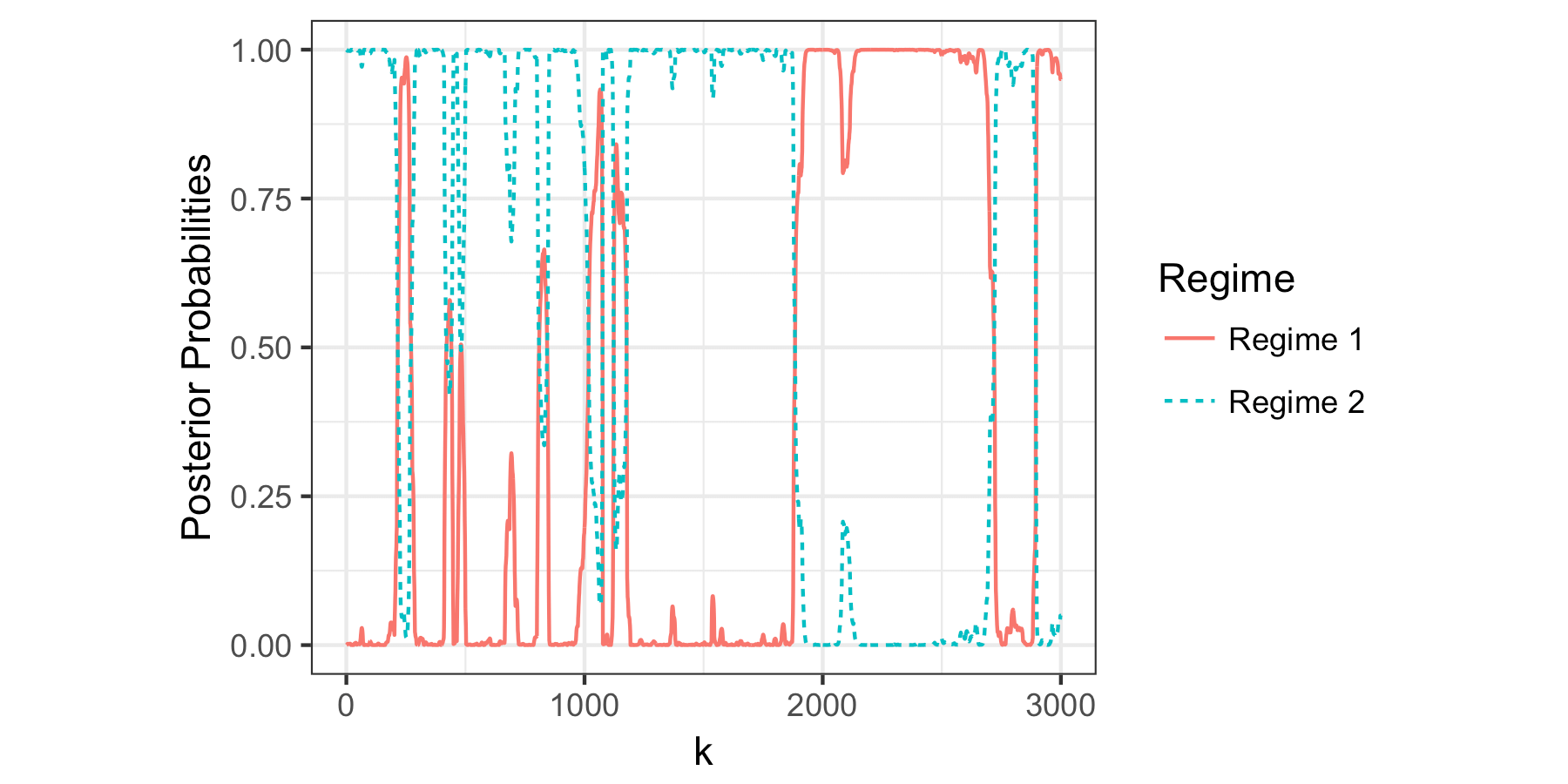 Figure 1
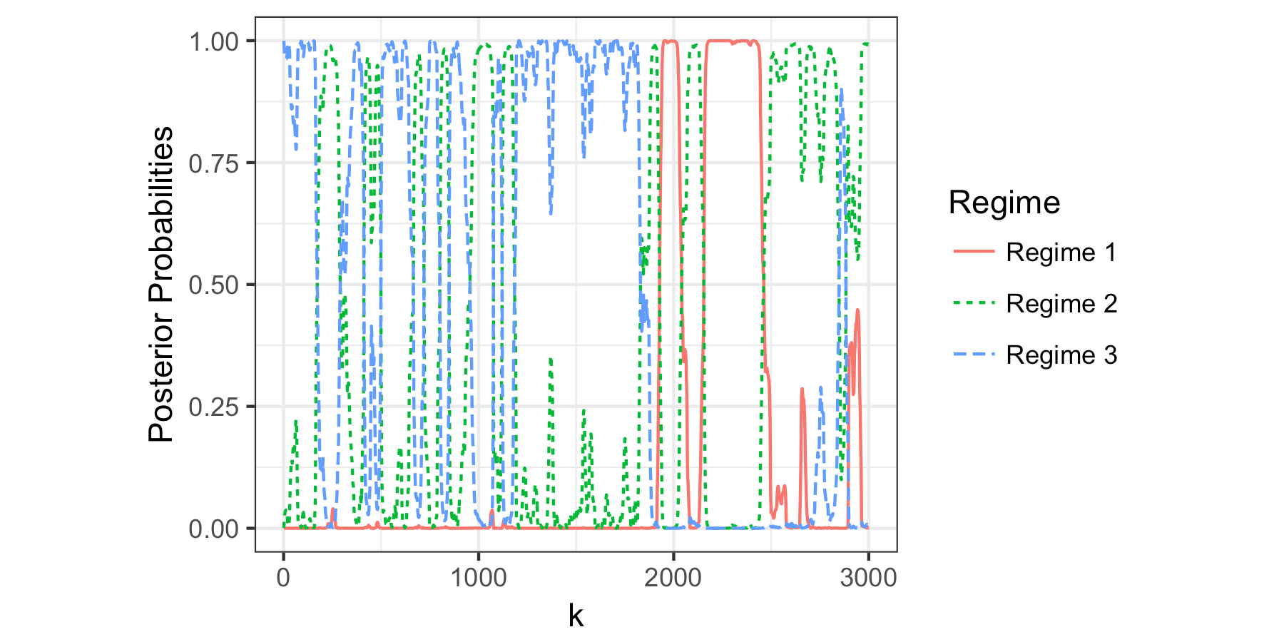 Figure 2