Chaotic Dynamics in Nonautonomous Maps: Application to the Nonautomous Henon Map
Francisco Balibrea-Iniesta, Carlos Lopesino, Stephen Wiggins, Ana, M. Mancho

TL;DR
This paper extends the theory of chaotic dynamics to nonautonomous two-dimensional maps, providing new conditions for chaos and hyperbolicity, exemplified through the nonautonomous Hénon map.
Contribution
It introduces a nonautonomous version of Conley-Moser conditions and derives a new sufficient condition for hyperbolic chaotic invariant sets in nonautonomous maps.
Findings
Established a precise definition of chaotic invariant sets for nonautonomous maps.
Derived new sufficient conditions for hyperbolic chaos in nonautonomous systems.
Applied the theory to the nonautonomous Hénon map to identify parameter regimes with chaotic behavior.
Abstract
In this paper we analyze chaotic dynamics for two dimensional nonautonomous maps through the use of a nonautonomous version of the Conley-Moser conditions given previously. With this approach we are able to give a precise definition of what is meant by a chaotic invariant set for nonautonomous maps. We extend the nonautonomous Conley-Moser conditions by deriving a new sufficient condition for the nonautonomous chaotic invariant set to be hyperbolic. We consider the specific example of a nonautonomous H\'enon map and give sufficient conditions, in terms of the parameters defining the map, for the nonautonomous H\'enon map to have a hyperbolic chaotic invariant set.
Click any figure to enlarge with its caption.
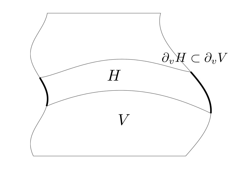 Figure 1
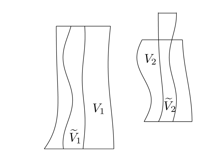 Figure 2
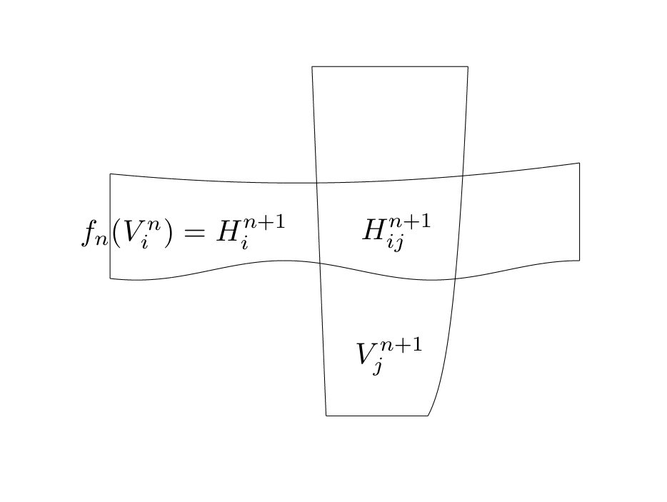 Figure 3
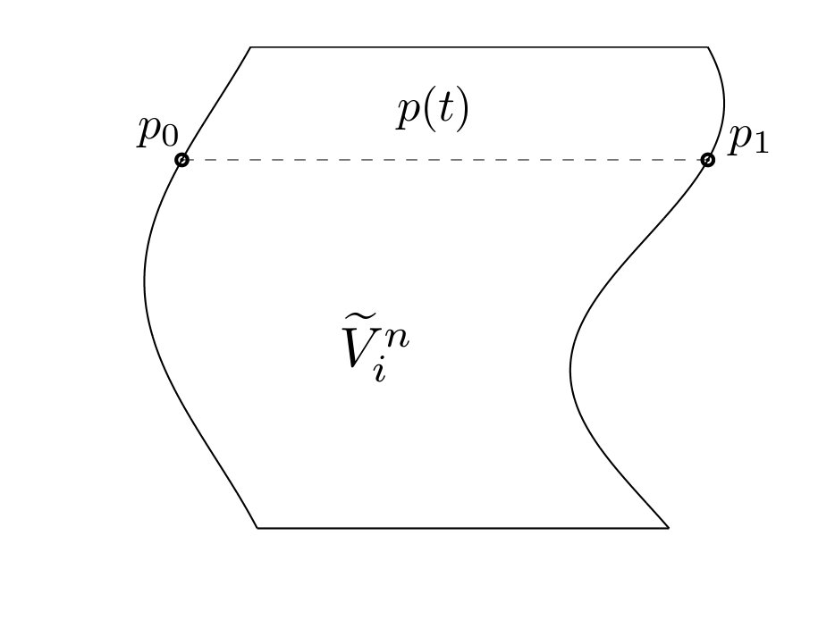 Figure 4
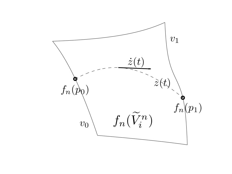 Figure 5
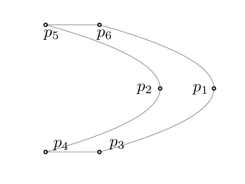 Figure 6
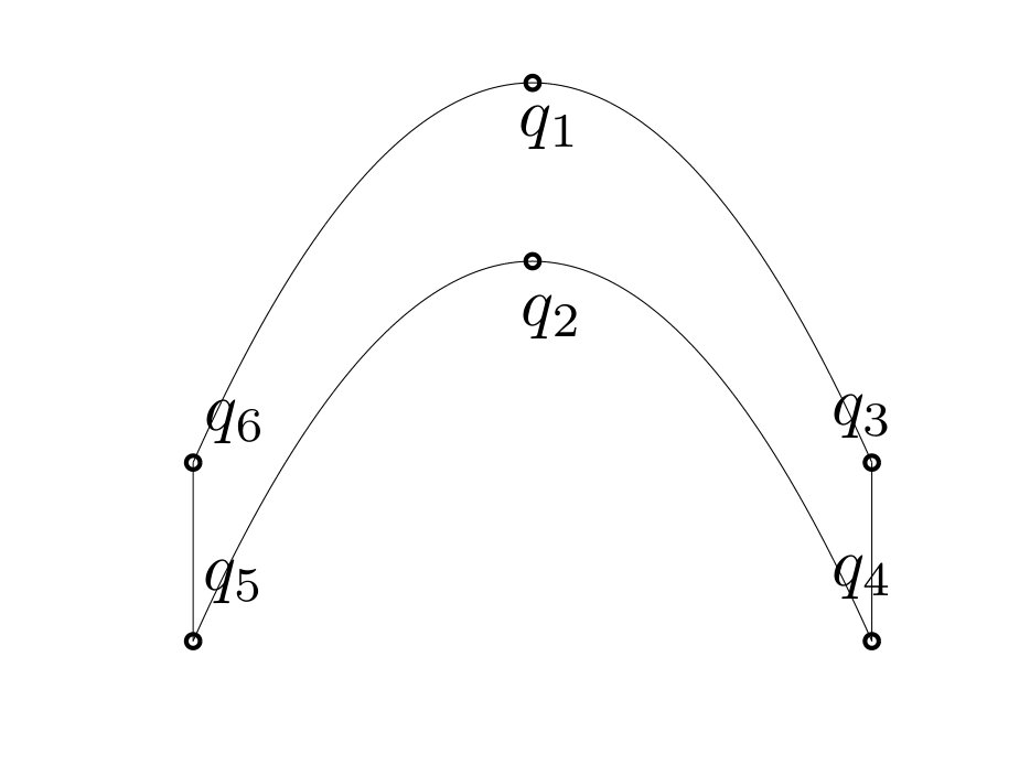 Figure 6
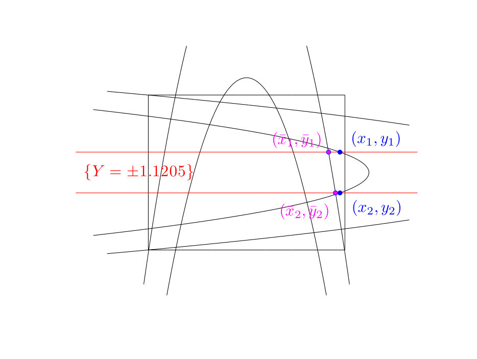 Figure 7
Peer Reviews
No public reviews on file for this paper yet. If you reviewed it on a platform where reviews are public (OpenReview, ICLR, NeurIPS, ICML), you can paste yours below so the community can read it here.
Videos
No videos yet. Explain this paper in a talk, walkthrough, or lecture? Add one.
\setkeys
Grotunits=360
CHAOTIC DYNAMICS IN NONAUTONOMOUS MAPS:
APPLICATION TO THE NONAUTONOMOUS HÉNON MAP
FRANCISCO BALIBREA-INIESTA111Instituto de Ciencias Matemáticas, CSIC-UAM-UC3M-UCM, Spain, [email protected].
Instituto de Ciencias Matemáticas, CSIC-UAM-UC3M-UCM,
C/ Nicolás Cabrera 15, Campus de Cantoblanco UAM
Madrid, 28049, Spain
CARLOS LOPESINO222Instituto de Ciencias Matemáticas, CSIC-UAM-UC3M-UCM, Spain, [email protected].
Instituto de Ciencias Matemáticas, CSIC-UAM-UC3M-UCM,
C/ Nicolás Cabrera 15, Campus de Cantoblanco UAM
Madrid, 28049, Spain
STEPHEN WIGGINS333School of Mathematics, University of Bristol, United Kingdom, [email protected].
School of Mathematics, University of Bristol,
Bristol BS8 1TW, United Kingdom
ANA M. MANCHO444Instituto de Ciencias Matemáticas, CSIC-UAM-UC3M-UCM, Spain, [email protected].
Instituto de Ciencias Matemáticas, CSIC-UAM-UC3M-UCM,
C/ Nicolás Cabrera 15, Campus de Cantoblanco UAM
Madrid, 28049, Spain
Abstract
In this paper we analyze chaotic dynamics for two dimensional nonautonomous maps through the use of a nonautonomous version of the Conley-Moser conditions given previously. With this approach we are able to give a precise definition of what is meant by a chaotic invariant set for nonautonomous maps. We extend the nonautonomous Conley-Moser conditions by deriving a new sufficient condition for the nonautonomous chaotic invariant set to be hyperbolic. We consider the specific example of a nonautonomous Hénon map and give sufficient conditions, in terms of the parameters defining the map, for the nonautonomous Hénon map to have a hyperbolic chaotic invariant set.
Keywords: chaotic dynamics, invariant set, hyperbolic.
1 Introduction
Studies of the Hénon map (Hénon [1976]) have played a seminal role in the development of our understanding of chaotic dynamics and strange attractors. The map depends on two parameters, and , and has the following form:
[TABLE]
where we will require in order to endure the existence of the inverse map,
[TABLE]
The “heart” of chaotic dynamics is exemplified by the so-called “Smale horseshoe map” (see Smale [1980] for a general description, with background). The essential feature of the Smale horseshoe map for chaos is that the map contains an invariant Cantor set on which the dynamics are topologically conjugate to a shift map defined on a finite number of symbols (a “chaotic invariant set”, sometimes also referred to as a “chaotic saddle”). Devaney and Nitecki [1979] gave sufficient conditions, in terms of the parameters and , for the Hénon map to have an invariant Cantor set on which it is topologically conjugate to a shift map of two symbols. The proof uses a technique due to Conley and Moser (see Moser [1973]) that is referred to as the “Conley-Moser conditions” (but for earlier work in a similar spirit see Alekseev [1968a, b, 1969]). Holmes [1982] used these conditions to show the existence of a chaotic invariant set in the so-called “bouncing ball map”. The Conley-Moser conditions were given a more detailed exposition, along with a slight weakening of the hypotheses, in Wiggins [2003]. More recently, the Conley-Moser conditions were used to show the existence of a chaotic invariant set in the Lozi map (Lopesino et al. [2015]).
The purpose of this paper is to carry out a similar analysis for a nonautonomous version of the Hénon map. The generalization of the Conley-Moser conditions for nonautonomous systems, i.e. in the discrete time setting with dynamics defined by an infinite sequence of maps, was given in Wiggins [1999]. We extend the nonautonomous Conley-Moser conditions further by providing an additional condition which is sufficient for the nonautonomous chaotic invariant set to be hyperbolic. Hyperbolicity of nonautonomous invariant sets is discussed in general in Katok and Hasselblatt [1995]. Earlier work on chaos in nonautonomous systems is described in Lerman and Silnikov [1992]; Stoffer [1988a, b]. Recent interesting work is described in Lu and Wang [2010, 2011].
While the development of the “dynamical systems approach to nonautonomous dynamics” is currently a topic of much interest, it is not a topic that is widely known in the applied dynamical systems community (especially the fundamental work that was done in the 1960’s). An applied motivation for such work is an understanding of fluid transport from the dynamical systems point of view for aperiodically time dependent flows. Wiggins and Mancho [2014] have given a survey of the history of nonautonomous dynamics as well as its application to fluid transport.
This paper is outlined as follows. In Section 2 we develop the required concepts for “building” chaotic invariant sets for two-dimensional nonautonomous maps. In Section 3 we prove the “main theorem” generalizing the Conley-Moser conditions that provide necessary conditions for two-dimensional nonautonomous maps to have a chaotic invariant set. In the course of the proof of the theorem the nature of chaotic invariant sets, and chaos, for nonautonomous maps is developed. This theorem was first given in Wiggins [1999], but in Section 3.1 we develop the theory further by providing a more analytical, rather than topological, construction for one of the Conley-Moser conditions that allows us to conclude that the nonautonomous chaotic invariant set is hyperbolic. In Section 4 we develop a version of the nonautonomous Hénon map and use the previously developed results to give sufficient conditions for the map to possess a nonautonomous chaotic invariant set. In Section 5 we discuss directions for future work along these lines.
2 Preliminary concepts
In this section we describe the basic setting and concepts that we will use throughout the remainder of the paper.
Nonautonomous dynamics will be defined by a sequence of maps and domains, , acting as follows:
[TABLE]
where, for our purposes, will be an appropriately chosen domain in , for all .
Similar to the Smale horseshoe construction (Wiggins [2003]), on each domain we must construct a finite collection of vertical strips ( and ) which map to a finite collection of horizontal strips located in :
[TABLE]
Associated with these mappings we will need to define a transition matrix as follows:
[TABLE]
[TABLE]
[TABLE]
However, first we must precisely define the notion of the domains that we will use, horizontal and vertical strips in those domains, and provide a characterization of the intersection of horizontal and vertical strips in the domain appropriate for our purposes.
To begin, let denote a closed and bounded set. We consider two associated subsets of :
[TABLE]
[TABLE]
Therefore and represent the projections of onto the -axis and the -axis respectively. From this it is easy to see that . We consider two closed intervals and . We next define -horizontal and -vertical curves on these domains.
Definition 2.1**.**
*Let . A -horizontal curve is defined to be the graph of a function where satisfies the following two conditions:
-
The set is contained in .
-
For every we have the Lipschitz condition*
[TABLE]
*Similarly, let . A -vertical curve is defined to be the graph of a function where satisfies the following two conditions:
-
The set is contained in .
-
For every we have the Lipschitz condition*
[TABLE]
Next we “fatten” these curves into strips.
Definition 2.2**.**
Given two nonintersecting -vertical curves , , we define a -vertical strip as
[TABLE]
Similarly, given two nonintersecting -horizontal curves , , we define a -horizontal strip as
[TABLE]
The width of horizontal and vertical strips is defined as
[TABLE]
We will need to consider different parts of the boundary of the strips in relation to the domain on which they are defined. The following three definitions provide the necessary concepts.
Definition 2.3**.**
The vertical boundary of a -horizontal strip is denoted
[TABLE]
The horizontal boundary of a -horizontal strip is denoted
[TABLE]
Definition 2.4**.**
We say that is a -horizontal strip contained in a -vertical strip if the two horizontal curves defining the horizontal boundaries of (denoted by ) are contained in , with the remaining boundary components of (denoted by ) contained in . These two last subsets, and are referred to as the horizontal and vertical boundaries of , respectively. See Figure 1.
Definition 2.5**.**
Let and be -vertical strips. is said to intersect fully if and . See Figure 2.
3 The main theorem
In this section we prove the main general theorem which provides sufficient conditions for the existence of a chaotic invariant set for nonautonomous maps. In the course of the proof our meaning of “chaos” for nonautonomous dynamics will be made precise.
Following the original development of the Conley-Moser conditions (Moser [1973]), there are three geometrical and analytical conditions that, if satisfied, provide sufficient conditions for an autonomous map (in the original formulation) to have a chaotic invariant set. These are referred to as A1, A2, and A3. The conditions A1 and A2 provide sufficient conditions for the existence of a topological chaotic invariant set. The conditions A1 and A3 provide sufficient conditions for a hyperbolic chaotic invariant set. Conditions A1 and A2 were developed for nonautonomous dynamics in Wiggins [1999]. In this section we recall A1 and A2, but we also give a new construction of A3 for nonautonomous dynamics555We point out a minor technical point. In previous development of the Conley-Moser conditions (e.g. Moser [1973]; Wiggins [2003]) the set-up considers the mapping of horizontal strips to vertical strips. However, for the Hénon map it is more natural to consider vertical strips mapping to horizontal strips. Of course, the choice of what we refer to as “horizontal” and “vertical” is arbitrary. However, the same choice of coordinate labeling as is used in the previous literature can be used for the Hénon map if we impose a rotation P=\left(\begin{array}[]{cc}0&1\\ 1&0\end{array}\right) on the sequence of maps or, alternatively, take each map as for every .. In particular, we will show that A1 and A3 imply that A1 and A2 also hold.
The following two lemmas will play an important role in the proof of the main theorem.
Lemma 3.1
*i) If is a nested sequence of -vertical strips with as , then is a -vertical curve.
ii) If is a nested sequence of -horizontal strips with as , then is a -horizontal curve.*
Lemma 3.2
Suppose . Then a -vertical curve and a -horizontal curve intersect in a unique point.
The proof of both these two lemmas can be found in Wiggins [2003].
We assume that for each we have:
[TABLE]
Furthermore, we assume that on each we can find a set of disjoint vertical strips, , such that each is one-to-one on . We then define
[TABLE]
with inverse function defined on for every , (see Figure 3).
The transition matrix is defined as follows:
[TABLE]
Now we can state the first two Conley-Moser conditions for a sequence of maps that are sufficient to prove the existence of a chaotic invariant set for nonautonomous systems.
Assumption 1** **(A1)
For all such that , is a -horizontal strip contained in with . Moreover, maps homeomorphically onto with .
Also, since maps homeomorphically onto with then maps homeomorphically onto () with
[TABLE]
Assumption 2** **(A2)
Let be a -vertical strip which intersects fully. Then is a -vertical strip intersecting fully for all such that . Moreover,
[TABLE]
Similarly, let be a -horizontal strip contained in such that also for some with . Then is a -horizontal strip contained in for all such that . Moreover,
[TABLE]
Now we develop symbolic dynamics in a form appropriate for nonautonomous dynamics. Let
[TABLE]
denote a bi-infinite sequence with () where adjacent elements of the sequence satisfy the rule , .
Similarly to the symbolic dynamics implemented for the Smale horseshoe (see page 575 of Wiggins [2003]), here we denote the set of all such symbol sequences by . If denotes the shift map
[TABLE]
on , we define the “extended shift map” on by
[TABLE]
Now we can state the main theorem.
Theorem 3.3** (Main theorem).**
Suppose satisfies A1 and A2. There exists a sequence of sets , with , such that the following diagram commutes
[TABLE]
where with a homeomorphism mapping onto .
Remark 3.4**.**
The sequence of sets is what we mean by a chaotic set for nonautonomous dynamics. Consequently our “main theorem” is a theoretical result which gives sufficient conditions for the existence of such a sequence of sets. The original proof can be found in Wiggins [1999], keeping in mind the geometrical considerations mentioned before.
Next, we will generalize the third Conley-Moser condition to the nonautonomous case. This will provide an alternative, and more analytical (as opposed to topological) method for proving that the second Conley-Moser condition holds, and it will also provide the additional information that the chaotic invariant set is hyperbolic.
3.1 Nonautonomous third Conley-Moser condition
We begin by giving a natural definition of stable and unstable sector bundles for the nonautonomous situation:
[TABLE]
[TABLE]
[TABLE]
[TABLE]
with being either or . Then we can state the following assumption: the third Conley-Moser condition for the nonautonomous setting.
Assumption 3** **(A3)
*, .
Moreover, if then*
[TABLE]
If then
[TABLE]
Obviously we need to impose an additional condition in order to guarantee the existence of the Jacobian matrices and . From now we will consider that for every on their respective domains. Now we establish an important relationship between assumptions A2 and A3.
Theorem 3.5**.**
If nonautonomous A1 and A3 are satisfied for then A2 is satisfied.
Part of the proof of this theorem is based on the following result.
Lemma 3.6
*Let be a sequence of maps satisfying A1 and A3.
For every and every pair of indices we have that
i) if is a -vertical curve, then is a -vertical curve in case .
ii) if is a -horizontal curve, then is a -horizontal curve in case .*
Proof 3.7**.**
*We omit the proof of ii) as it follows the same line of reasoning as i).
We consider a -vertical curve . By definition there exist an interval and a function such that is the graph of and also the Lipschitz condition holds for a constant and every pair of points .
It follows from Assumption 1 that is a homeomorphism over . In particular a homeomorphism over . This implies that*
[TABLE]
Since the curve can be parametrized by (take also ) then this last subset can also have a parametrization but over a smaller domain ,
[TABLE]
The image of ant tangent vector of under has the form
[TABLE]
This last relation follows directly from the Lipschitz condition:
[TABLE]
By applying Assumption 3 we obtain that the tangent vectors belong to ,
[TABLE]
Moreover, as we also assume that , any tangent vector
[TABLE]
From these two relations it follows that cannot change its sign in the entire domain . Consequently for every pair of points there exist such that , and we have the inequality
[TABLE]
[TABLE]
and this result implies that is a -vertical curve.
Proof 3.8** (Proof of Theorem 3.5).**
*The theorem will be proved by verifying the following steps.
Step 1: Let be a -vertical curve. Then is a -vertical curve for every such that .
Step 2: Let be a -vertical strip which intersects fully. Then is a -vertical strip that intersects fully for every such that .
Step 3: Show that for .
We omit the part of the proof dealing with horizontal strips since it follows from the same reasoning used to prove the part concerning vertical strips.
We begin with Step 1. Let be a -vertical curve. For each such that , by applying A1 we obtain that is a -horizontal strip contained in . Since implicitly we are taking as one of the two components of the vertical boundary of a vertical strip intersecting fully, the curve intersects in exactly two points.
Also because maps the horizontal boundaries of each subset onto the horizontal boundaries of , we have that is a curve linking the two horizontal boundaries of . Finally if we apply Lemma 3.6 to this curve it follows that is also a -vertical curve.
*To prove Step 2 we apply Step 1 to the -vertical boundaries of the -vertical strip which intersects fully. It then follows that is also a -vertical strip for every such that . Moreover this last strip intersects each fully because of the geometric considerations in Step 1.
For proving Step 3 first we need to fix an iteration and an index . The width of each -vertical strip will be the distance between two points with the same -component and located in separate vertical boundaries, .*
By taking segment considered in Figure 4, is a vector with its -component equal to zero. Therefore , . Now we have that the curve located in is a -horizontal curve because of the second part of Lemma 3.6,
[TABLE]
Furthermore since the graph of is a -horizontal curve, we obtain that
[TABLE]
by denoting for .
Using this last fact and also the geometric considerations in Figure 5, it follows that
[TABLE]
[TABLE]
[TABLE]
Also as a result of the last part of Assumption 3 there exists a positive constant , which we impose to be , such that
[TABLE]
[TABLE]
*Note that the two expressions containing the integrals are equal since does not change its sign at any point. This is due to the fact that the graph of is a -horizontal curve.
Finally we arrive at the result,*
[TABLE]
[TABLE]
4 Nonautonomous Hénon map
We have now developed the necessary tools for proving the existence of a chaotic invariant set for the nonautonomous Hénon map. Recall our general notation for nonautonomous dynamics (a sequence of maps defined on a sequence of domains), .
We will construct domains for the nonautonomous Hénon map, each of them containing an associated pair of horizontal strips and another of vertical strips. Moreover, the transition matrices will be shown to be identical for each map , with A=\left(\begin{array}[]{cc}1&1\\ 1&1\end{array}\right) for each iteration .
Recall that the autonomous Hénon map has the form:
[TABLE]
Following Devaney and Nitecki [1979], sufficient conditions for the existence of a chaotic invariant set in the autonomous context can be proven when the parameters satisfy the following inequalities:
[TABLE]
Note that when the map is orientation-preserving and area-preserving. For our version of the nonautonomous Hénon map, we will take for the sequence of maps in order to retain these properties, but we will allow to vary for each iteration . Therefore, we will take:
[TABLE]
where
[TABLE]
This choice is motivated by the fact that is the minimum threshold for parameter for which the autonomous Hénon map satisfies the autonomous versions of Assumptions 1 and 3 of the Conley-Moser conditions.
In the following we will prove that the nonautonomous Hénon map satisfies the conditions described in Theorem 3.3. In particular, we will prove the following theorem.
Theorem 4.1**.**
If then the nonautonomous Hénon map with , has a nonautonomous chaotic invariant set in .
Proof 4.2**.**
*We carry out the proof for the specific case where . The case for follows similar reasoning as for the case , with the main difference being that some values in the inequalities appearing when checking Assumption 3 must be changed. We begin with the first Conley-Moser condition.
Assumption 1. The domain on which each function will be defined is the square*
[TABLE]
*analogously to the domain considered for the autonomous Hénon map.
The horizontal strips and the vertical strips associated to any iteration will be taken as*
[TABLE]
and since is a homeomorphism we also note that vertical strips “move” to horizontal strips in forward iteration,
[TABLE]
*Moreover the index indicating the number of strips in either or is and the strips are defined by
[TABLE]
[TABLE]
*These are determined by the images of with respect to and for every . They result easy to compute. Let
[TABLE]
[TABLE]
the segments which conform the boundary of . Their images with respect and are either another segment or a parabola, and as is a homeomorphism, both and are two strips with a parabolic form.
The key points of and shown in Figure 6 have the following coordinates,
[TABLE]
[TABLE]
[TABLE]
[TABLE]
The coordinates of the these points satisfy , and
[TABLE]
with strict inequality when . Only in case , the points are inside the domain and actually these are three vertices of the square . In any case, it follows that the points and do not belong to for any .
We denote the arguments of the parabolic curves by and , so that their equations take the form:
[TABLE]
[TABLE]
With this notation the absolute value of the derivatives of these functions take the form:
[TABLE]
and their maximum values are assumed when and , respectively. Therefore we have:
[TABLE]
*Due to reasons explained later, for convenience we will choose the thresholds for the maximum values that the slopes of the horizontal and vertical boundaries can assume, respectively. Using this fact, one can conclude that is a -horizontal strip and a -vertical strip for every and . Moreover, . This proves part of Assumption 1.
Furthermore, for any and we have that the horizontal boundaries of are two -horizontal curves which link the left and right sides of the square . Since the two -vertical curves bounding link the upper and the bottom sides of , both boundaries and intersect in four different points. From this fact it follows that is a -horizontal strip contained in .
Since is a homeomorphism for every ,*
[TABLE]
[TABLE]
*This can be checked by an easy computation.
Therefore the nonautonomous Hénon map satisfies Assumption 1.
Assumption 3. To begin our verification that A3 is also satisfied, we need to recall the notation for several concepts developed earlier:*
[TABLE]
[TABLE]
[TABLE]
*with being either or .
Now given any point and any (which by definition, ) we have that*
[TABLE]
belongs to if and only if the inequality
[TABLE]
Since it is also true that
[TABLE]
[TABLE]
*In case , the previous inequality (55) will hold.
To verify this we need to check if*
[TABLE]
*At this point we give a geometrical argument.
The horizontal lines cut the parabola at two points:*
[TABLE]
[TABLE]
* The horizontal lines cut the parabola at two points with a positive -component:*
[TABLE]
[TABLE]
From here we have that
[TABLE]
[TABLE]
[TABLE]
The inequalities (note that is trivial due to the definitions) also hold for every parameter satisfying and . The reason comes from comparing the derivatives of and with respect to :
[TABLE]
[TABLE]
[TABLE]
[TABLE]
[TABLE]
Clearly for every . It follows that for .
*This setup shows that every point satisfies that , since the four areas composing are either beneath the line or above the line , as can be observed in Fig. 7.
*Since is an arbitrary point, the inclusion is proven. *
*For the second inclusion we focus on the fact that and since transforms the -components of the points of into the -components of the points of , it immediately follows that *
[TABLE]
[TABLE]
As in the previous case this inequality allows us to prove the inclusion,
[TABLE]
[TABLE]
[TABLE]
[TABLE]
[TABLE]
[TABLE]
*and then the inclusion is proved.
Finally for the last part of Assumption 3 we will only prove the inequality*
[TABLE]
since the inequality
[TABLE]
*is proved by using the same argument.
[TABLE]
[TABLE]
[TABLE]
This last inequality is true if we require that . This interval exists since is less than . Then we have that
[TABLE]
Analogously for any ,
[TABLE]
*and the proof that the nonautonomous Hénon map satisfies A1 and A3 with is complete. Consequently it also satisfies A2 by using Theorem 3.5.
By applying the main theorem it follows that there exists a chaotic invariant set (with respect to the nonautonomous Hénon map ) contained in (let say and ) which is conjugate to a shift map of two symbols.*
Remark 4.3**.**
*Comparing this result to what happens for the autonomous Hénon map, it is curious that for some the quantity is less than , which is the minimum threshold for parameter for which the autonomous Hénon map satisfies the autonomous Assumption 3.
In other words, this given example shows that although for some the values that parameter takes imply that does not satisfy the autonomous Assumption 3 separately, this fact does not necessarily mean that the nonautonomous Assumption 3 is not satisfied for the sequence .*
5 Summary and Conclusions
In this paper we have considered a nonautonomous version of the Hénon map and have provided necessary conditions for the map to possess a nonautonomous chaotic invariant set. This is accomplished by using a nonautonomous version of the Conley-Moser conditions given in Wiggins [1999]. We sharpen these conditions by providing a more analytical condition that, as a consequence, enables us to show that the chaotic invariant set is hyperbolic. In the course of the proof we provide a precise characterization of what is mean by the phrase “hyperbolic chaotic invariant set” for nonautomous dynamical systems. Currently there is much interest in nonautomous dynamics and a thorough analysis of a specific example might provide a benchmark for further studies, just as the work in Devaney and Nitecki [1979] provided a benchmark for studies of chaotic dynamics for autonomous maps. Indeed, our generalization of the Hénon map to the nonautonomous setting provides an approach to generalizing the map to even more general nonautonomous settings, such as a consideration of “noise”. This would be an interesting topic for future studies.
Acknowledgments
The research of FB-I, CL and AMM is supported by the MINECO under grant MTM2014-56392-R. The research of SW is supported by ONR Grant No. N00014-01-1-0769. We acknowledge support from MINECO: ICMAT Severo Ochoa project SEV-2011-0087.
The reference list from the paper itself. Each links out to its DOI / PubMed record.
- 1Alekseev [1968 a] Alekseev, V.M. (1968 a). Quasirandom dynamical systems, I. Math. USSR-Sb , 5 , 73-128.
- 2Alekseev [1968 b] Alekseev, V.M. (1968 b). Quasirandom dynamical systems, II. Math. USSR-Sb , 6 , 505-560.
- 3Alekseev [1969] Alekseev, V.M. (1969). Quasirandom dynamical systems, III. Math. USSR-Sb , 6 , 1-43.
- 4Devaney and Nitecki [1979] Devaney, R. L., Nitecki, Z. (1979). Shift automorphisms in the Hénon mapping. Comm. Math. Phys. , 67 , 137-179.
- 5Hénon [1976] Hénon, M. (1976). A Two-Dimensional Mapping with a Strange Attractor. Comm. Math. Phys. , 50 , 69-77.
- 6Holmes [1982] Holmes, P.J. (1982). The dynamics of repeated impacts with a sinusoidally vibrating table. Journal of Sound and Vibration, 84(2) , 173-189.
- 7Katok and Hasselblatt [1995] Katok, A. and Hasselblatt, B. (1995). Introduction to the Modern Theory of Dynamical Systems . Cambridge University Press, Cambridge.
- 8Lerman and Silnikov [1992] Lerman, L. and Silnikov, L. (1992). Homoclinical structures in nonautonomous systems: Nonautonomous chaos. Chaos , 2 , 447–454.