A Theoretical Framework for Lagrangian Descriptors
Carlos Lopesino, Francisco Balibrea-Iniesta, V\'ictor J., Garc\'ia-Garrido, Stephen Wiggins, Ana M. Mancho

TL;DR
This paper establishes a rigorous theoretical foundation for Lagrangian Descriptors (LDs), proving their effectiveness in detecting invariant manifolds and other phase space structures in various dynamical systems.
Contribution
It introduces an alternative definition for LDs and rigorously proves their ability to identify stable and unstable manifolds in specific 2D hyperbolic saddle cases, extending to invariant sets like n-tori.
Findings
LDs reliably detect invariant manifolds in 2D hyperbolic saddle points.
LDs can highlight additional invariant sets such as n-tori.
Application to classical examples demonstrates the method's effectiveness.
Abstract
This paper provides a theoretical background for Lagrangian Descriptors (LDs). The goal of achieving rigourous proofs that justify the ability of LDs to detect invariant manifolds is simplified by introducing an alternative definition for LDs. The definition is stated for -dimensional systems with general time dependence, however we rigorously prove that this method reveals the stable and unstable manifolds of hyperbolic points in four particular 2D cases: a hyperbolic saddle point for linear autonomous systems, a hyperbolic saddle point for nonlinear autonomous systems, a hyperbolic saddle point for linear nonautonomous systems and a hyperbolic saddle point for nonlinear nonautonomous systems. We also discuss further rigorous results which show the ability of LDs to highlight additional invariants sets, such as -tori. These results are just a simple extension of the ergodic…
Click any figure to enlarge with its caption.
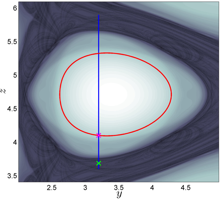 Figure 10
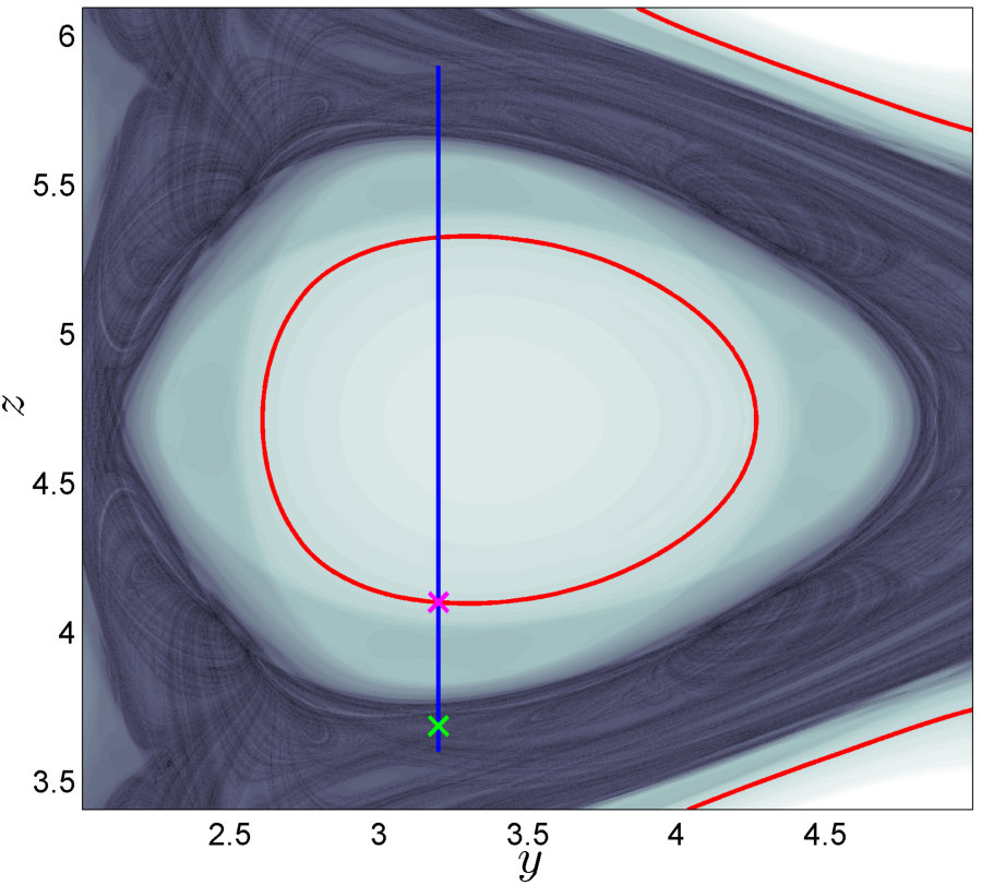 Figure 10
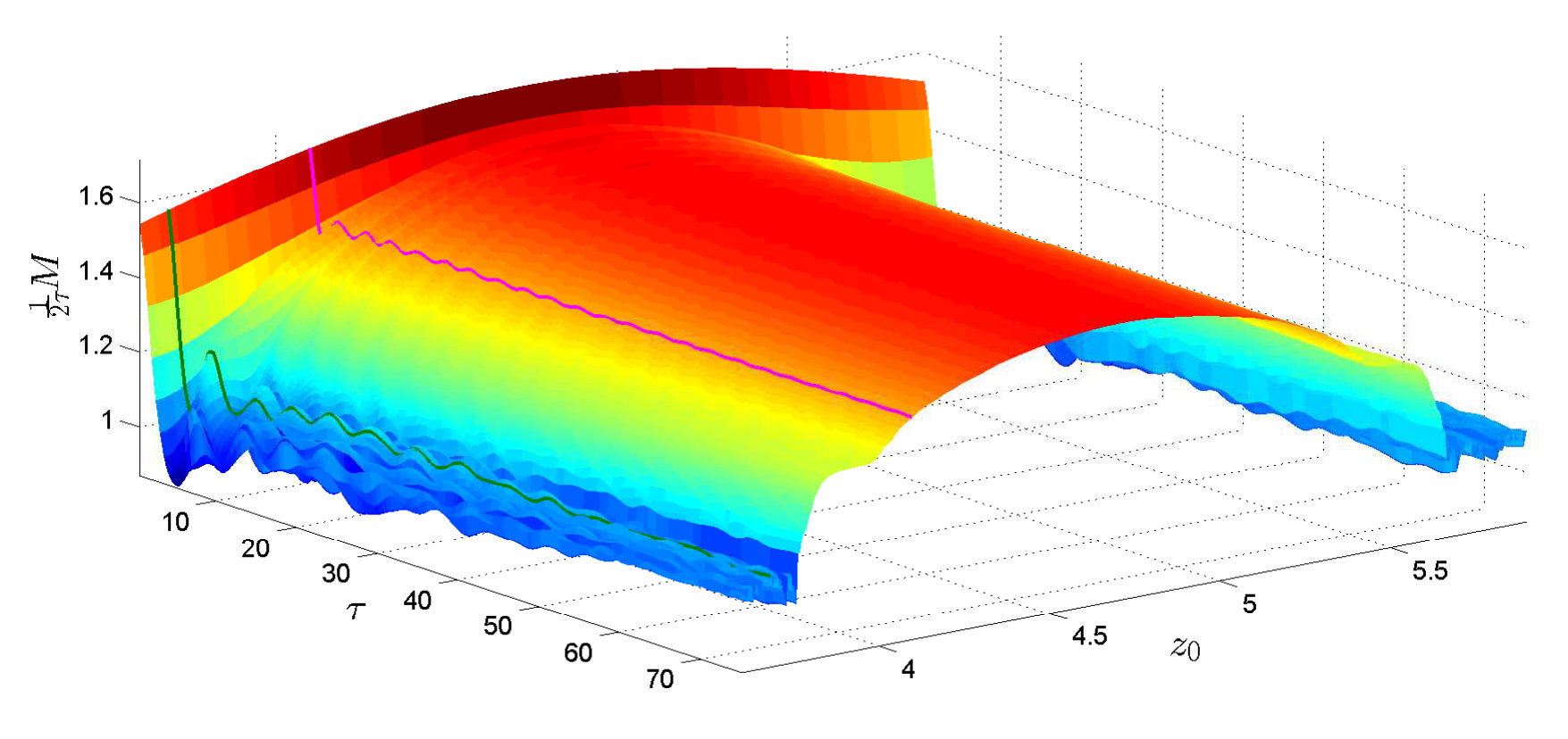 Figure 11
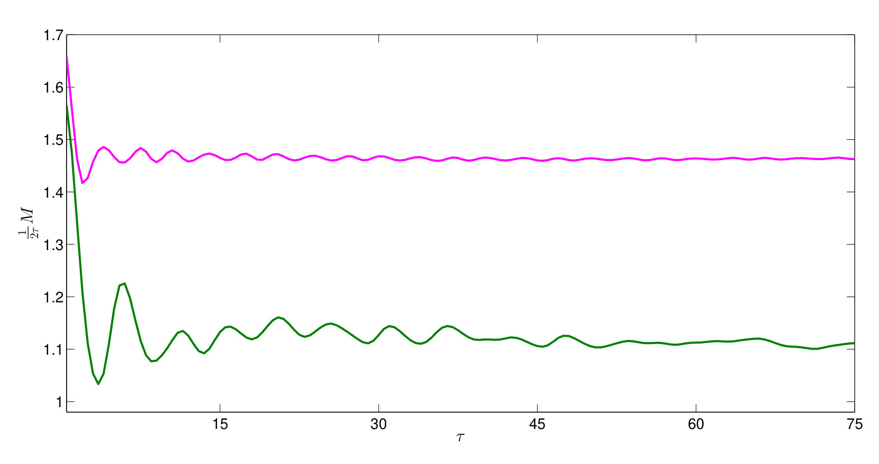 Figure 11
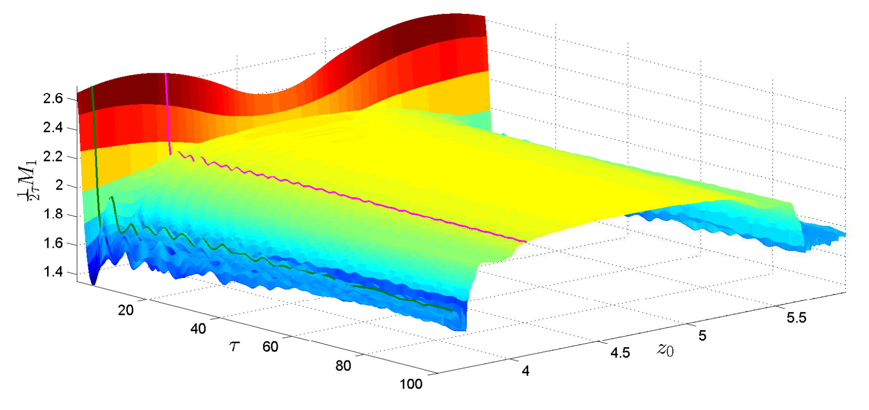 Figure 12
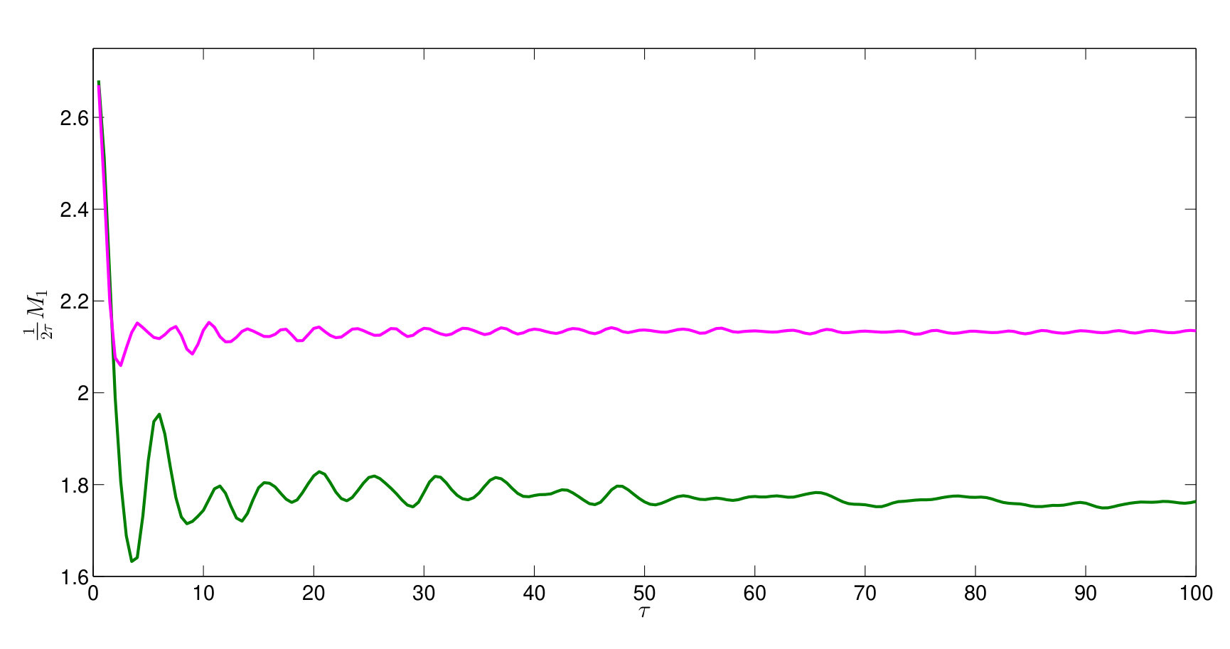 Figure 12
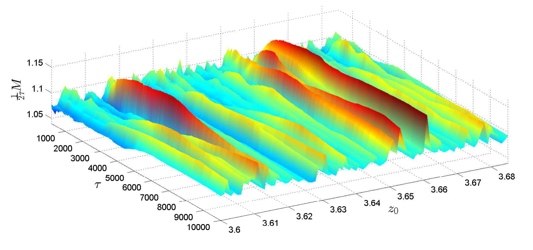 Figure 13
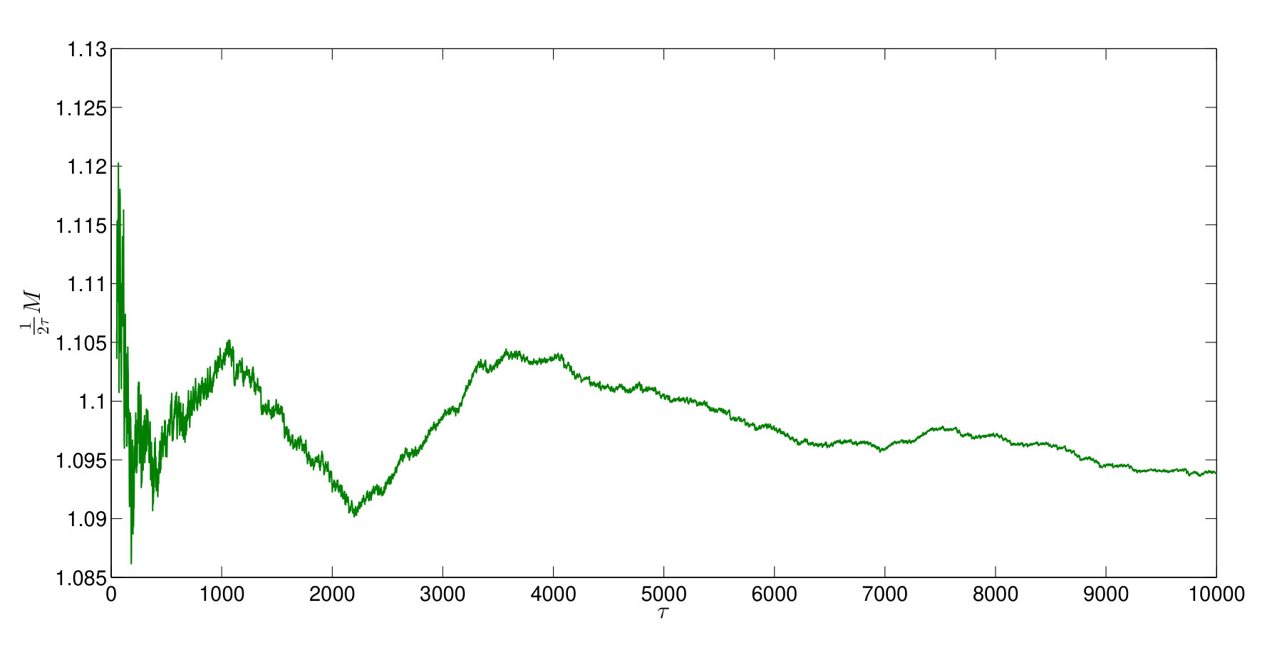 Figure 13
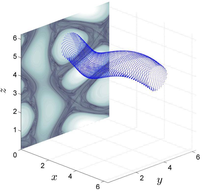 Figure 14
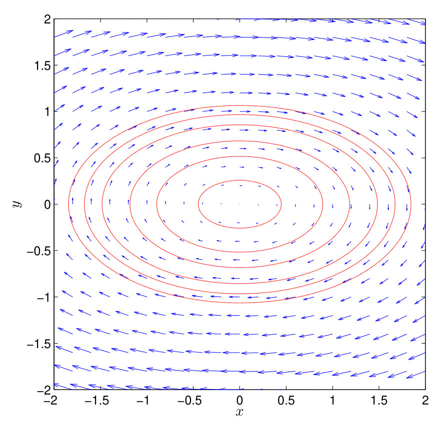 Figure 15
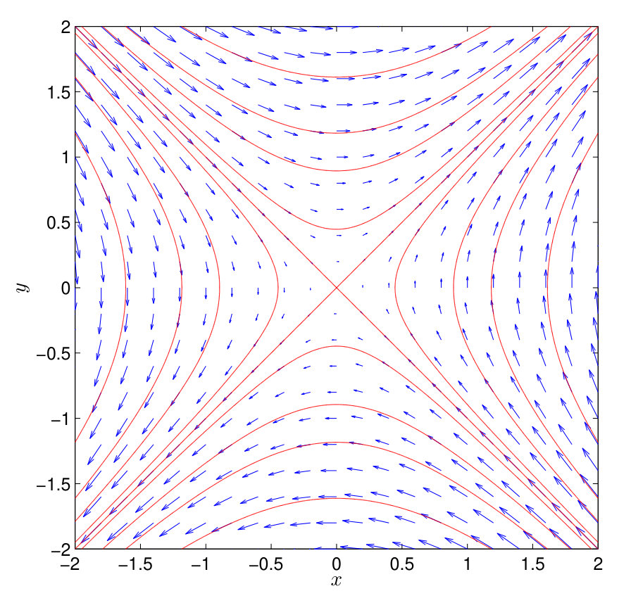 Figure 15
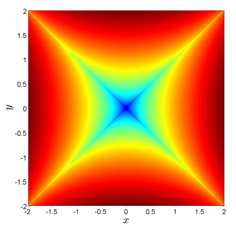 Figure 16
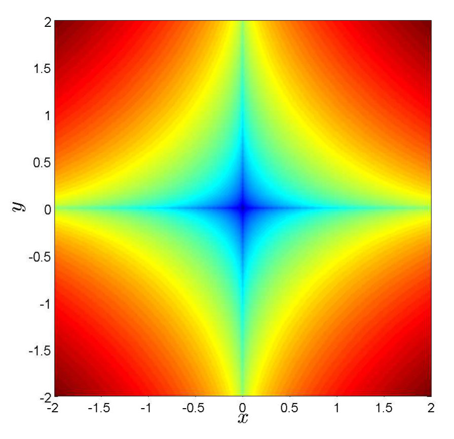 Figure 16
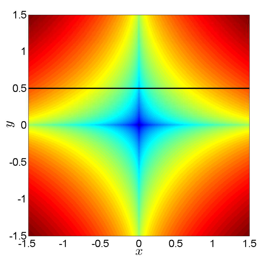 Figure 1
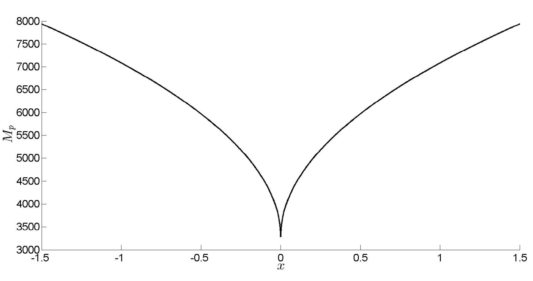 Figure 1
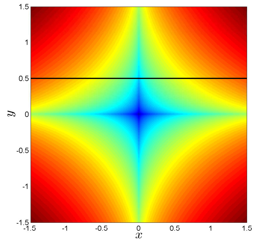 Figure 2
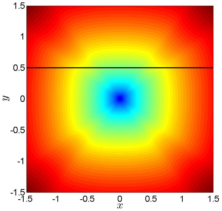 Figure 2
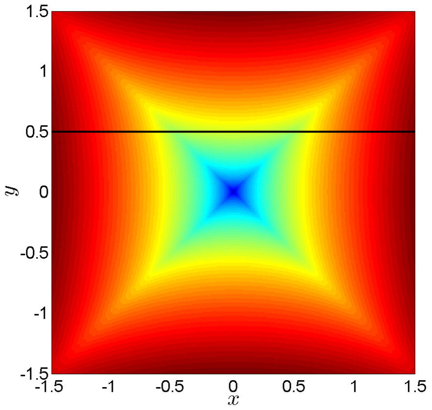 Figure 2
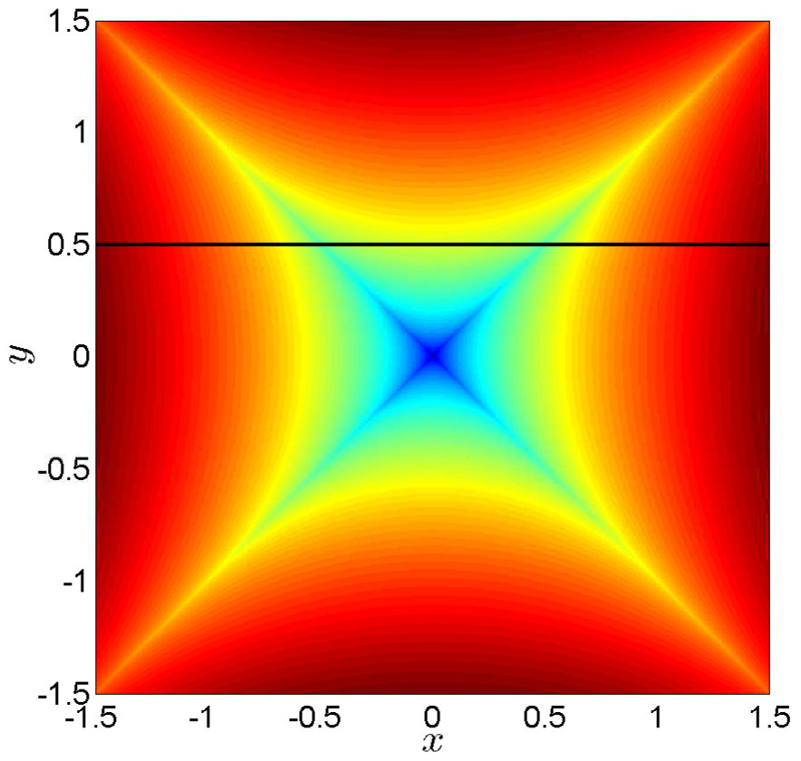 Figure 2
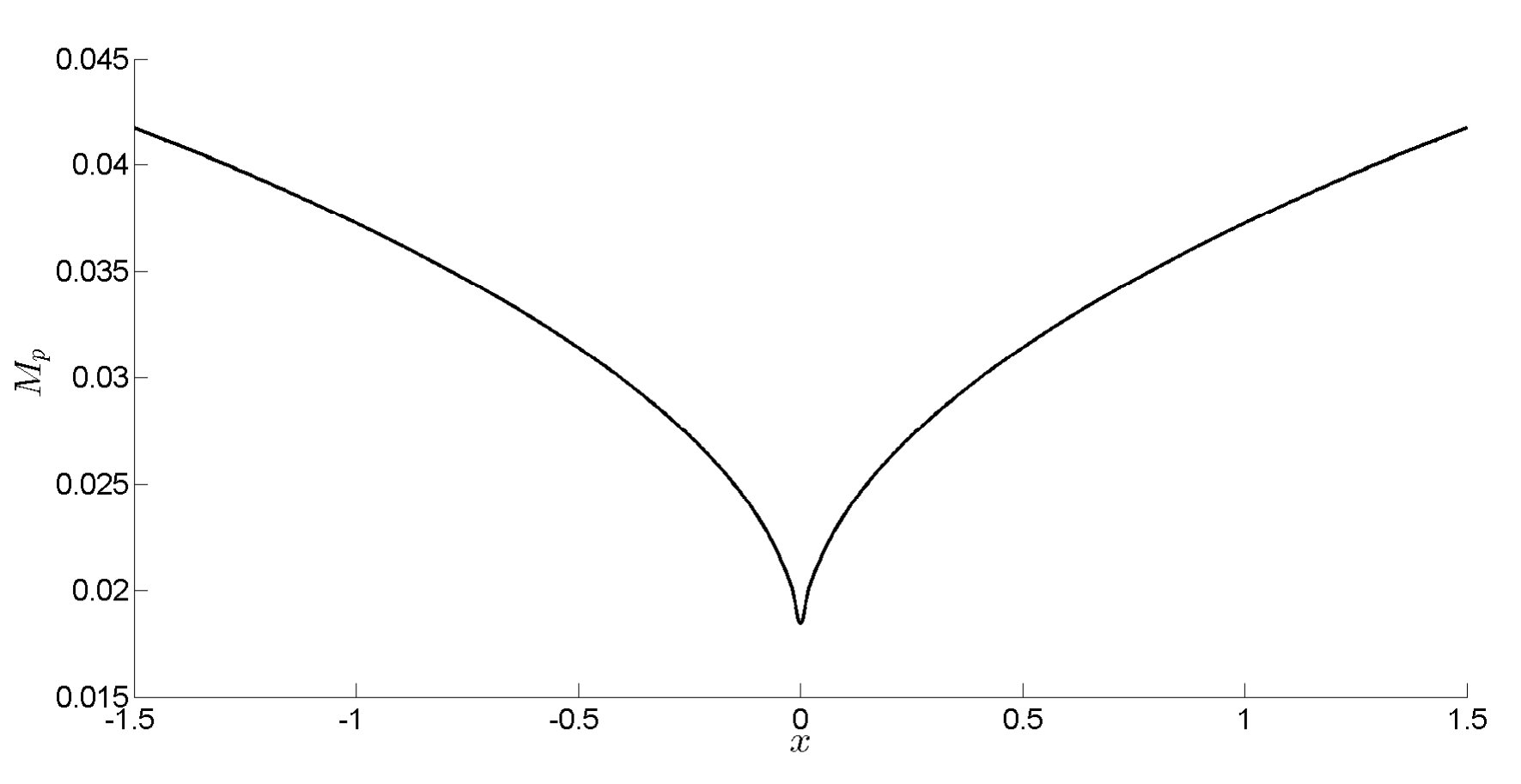 Figure 3
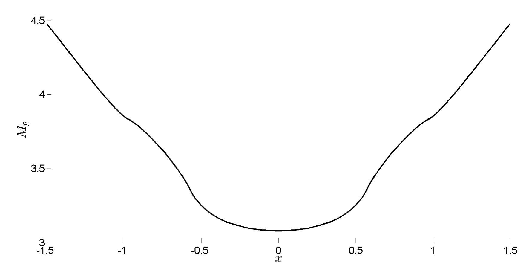 Figure 3
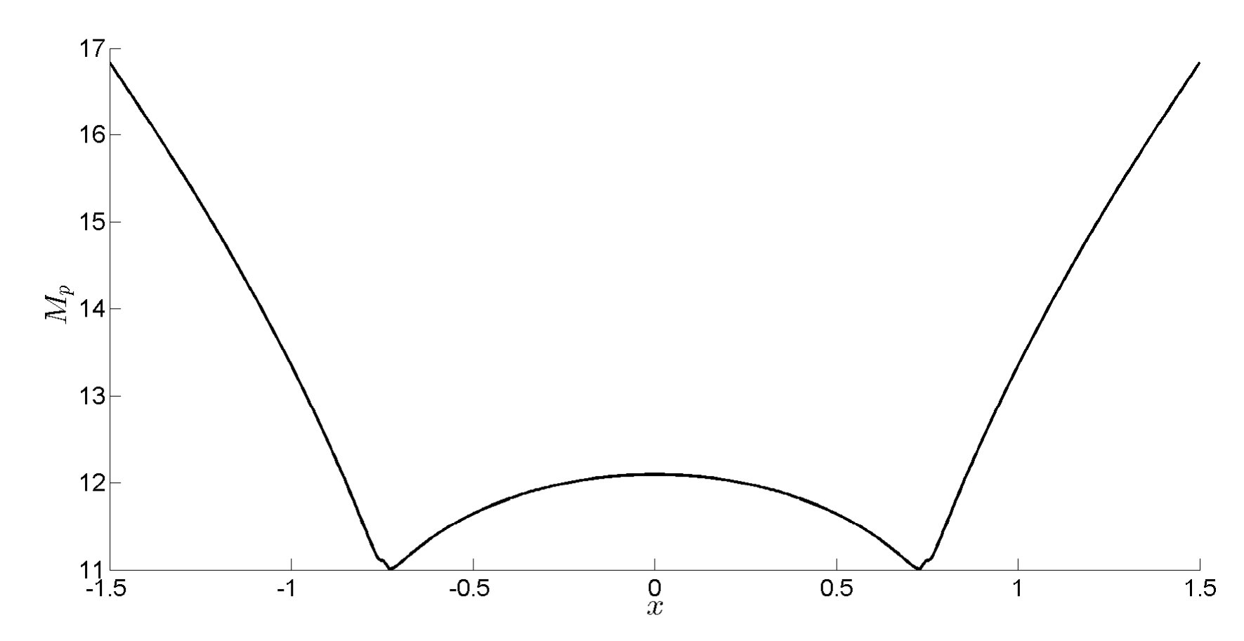 Figure 3
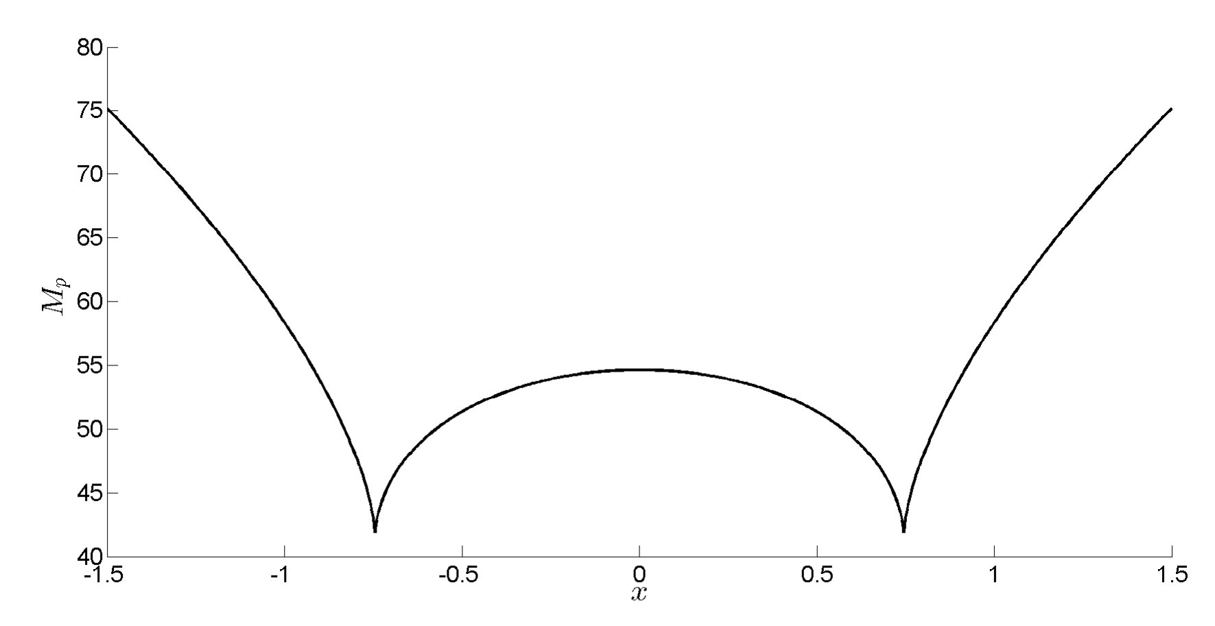 Figure 3
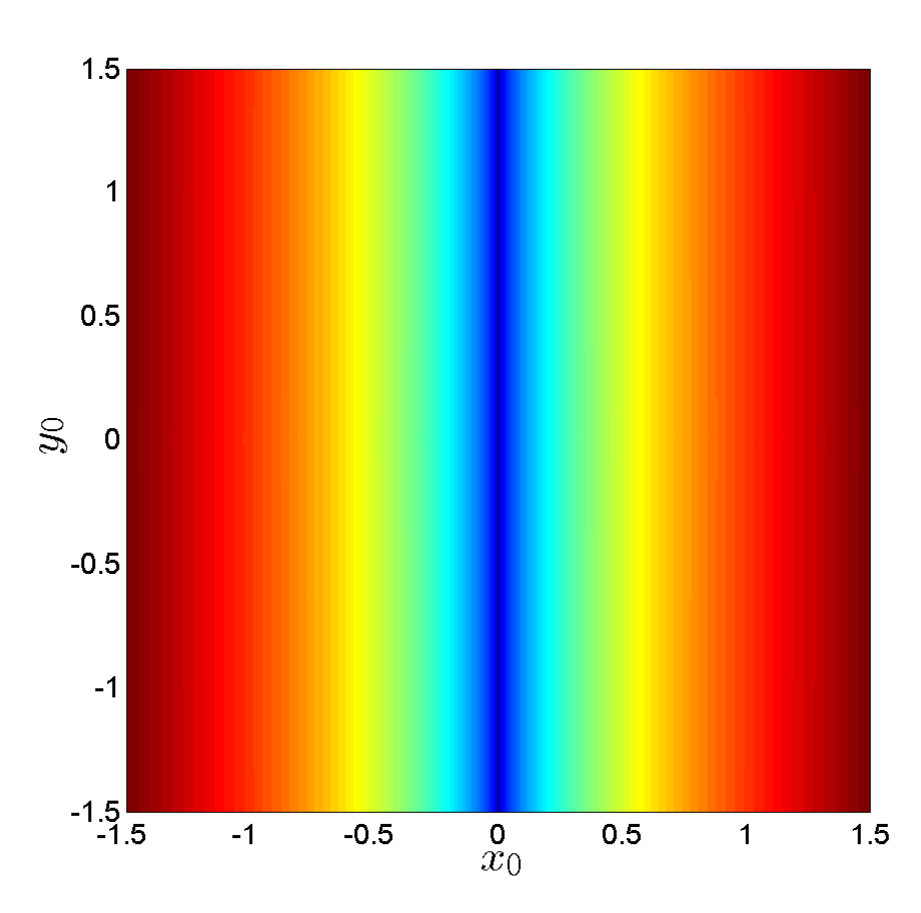 Figure 4
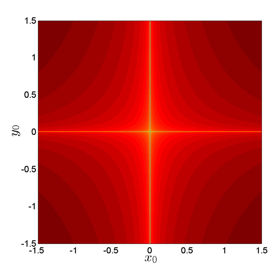 Figure 4
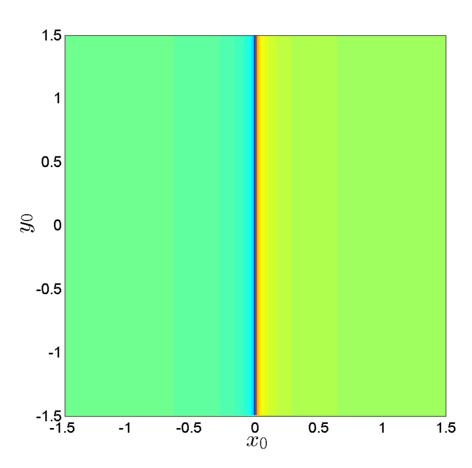 Figure 5
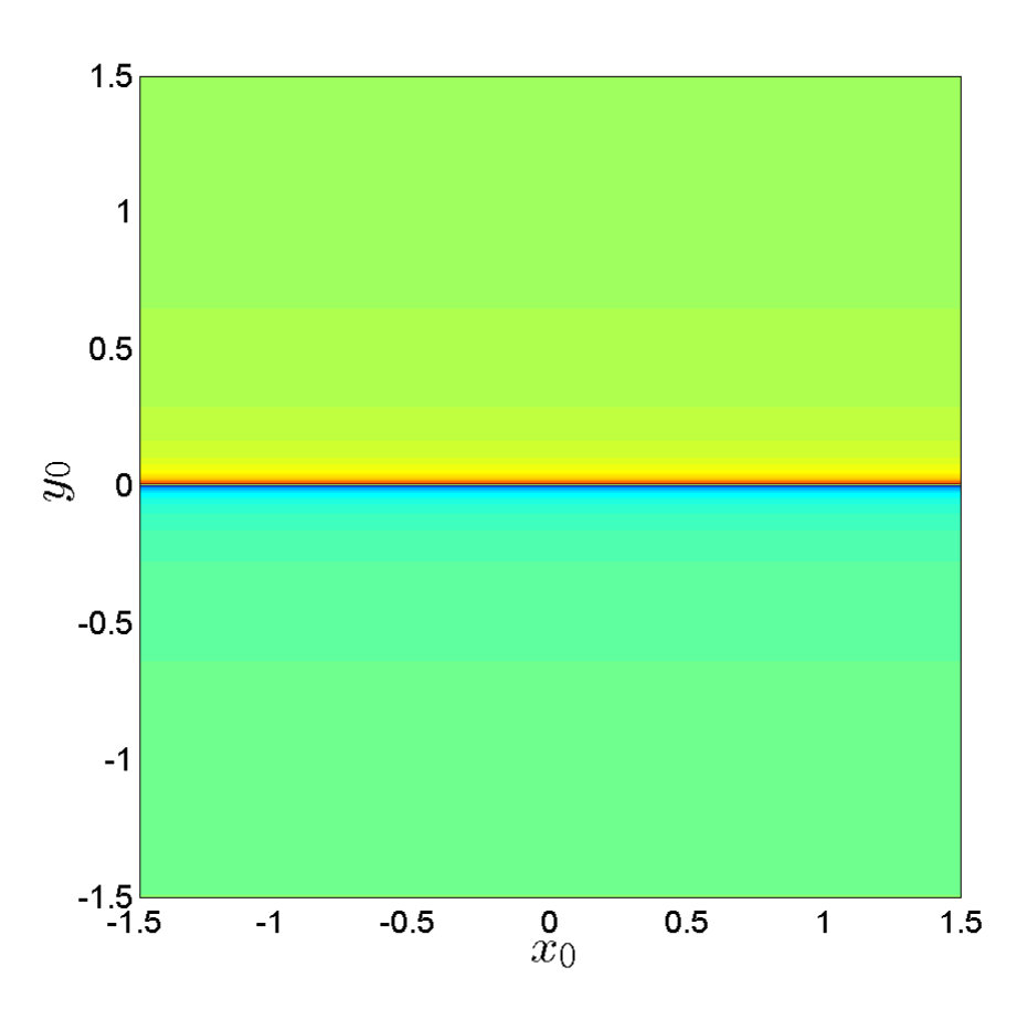 Figure 5
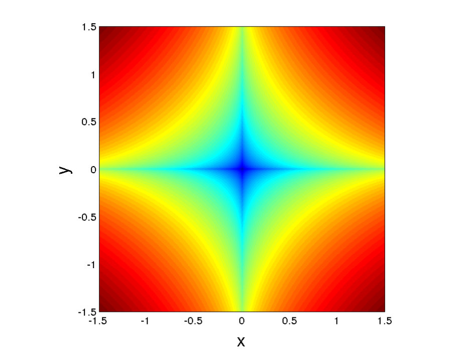 Figure 6
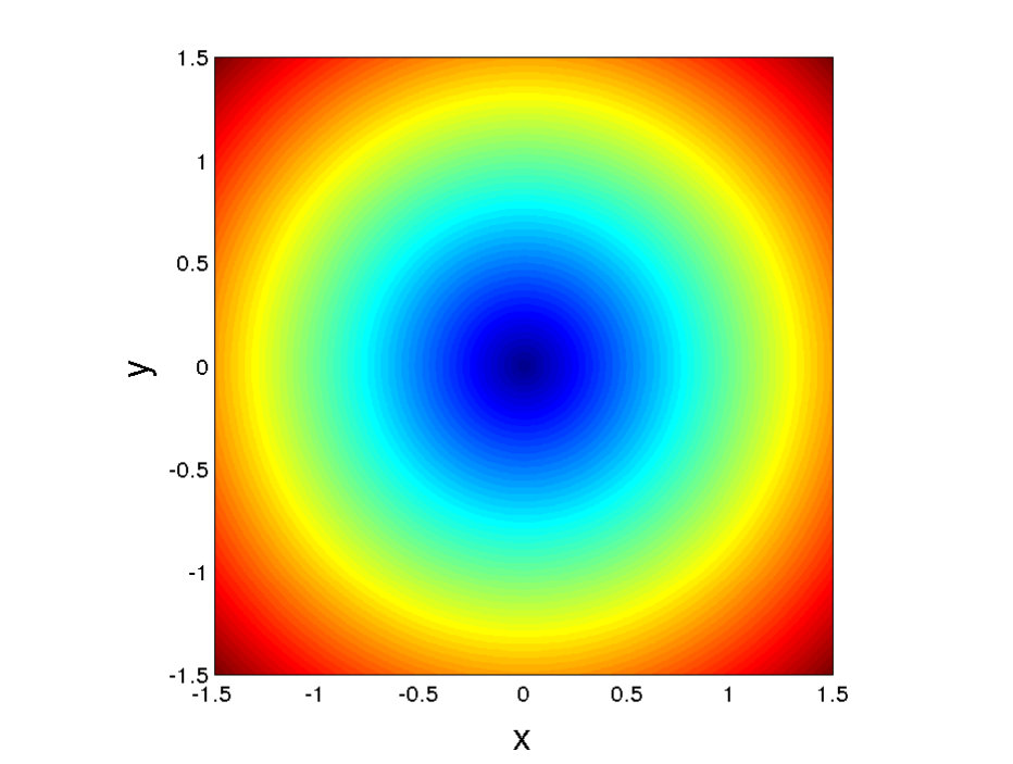 Figure 6
 Figure 7
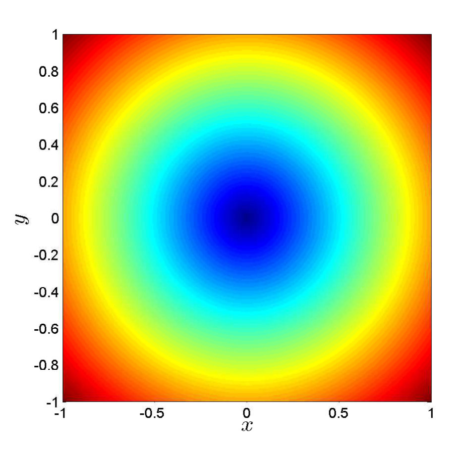 Figure 7
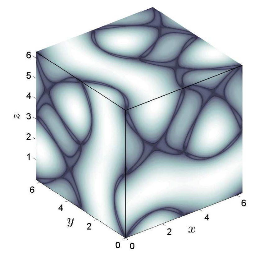 Figure 8
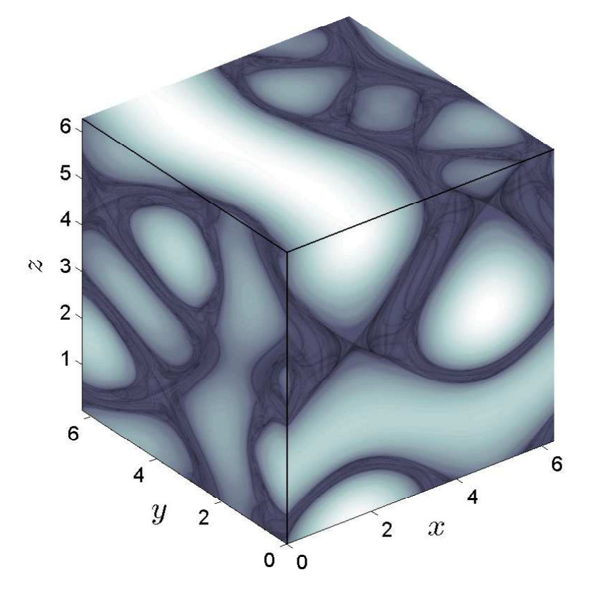 Figure 8
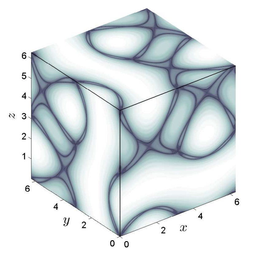 Figure 8
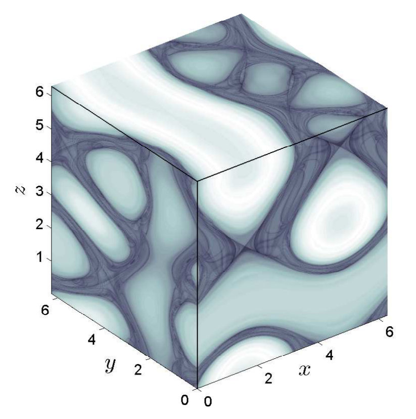 Figure 8
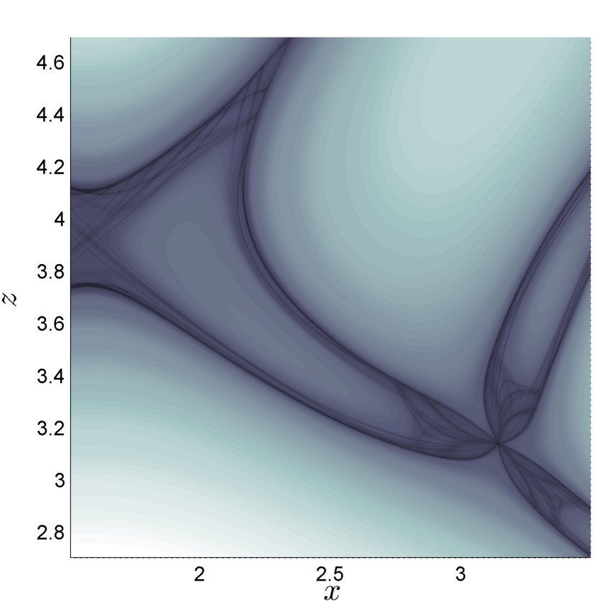 Figure 9
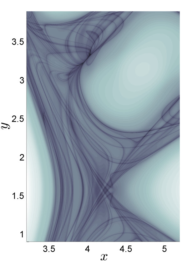 Figure 9
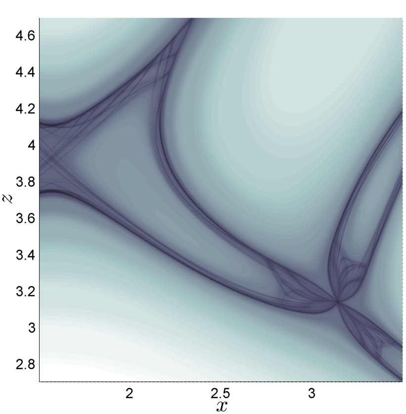 Figure 9
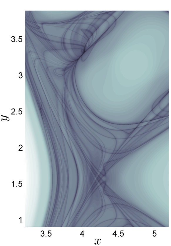 Figure 9
Peer Reviews
No public reviews on file for this paper yet. If you reviewed it on a platform where reviews are public (OpenReview, ICLR, NeurIPS, ICML), you can paste yours below so the community can read it here.
Videos
No videos yet. Explain this paper in a talk, walkthrough, or lecture? Add one.
\setkeys
Grotunits=360
A Theoretical Framework for Lagrangian Descriptors
C. Lopesino1
F. Balibrea-Iniesta1
V. J. García-Garrido1
S. Wiggins2
A. M. Mancho1
1Instituto de Ciencias Matemáticas
CSIC-UAM-UC3M-UCM
C/Nicolás Cabrera 15
Campus Cantoblanco UAM
28049 Madrid
Spain
2School of Mathematics
University of Bristol
Bristol BS8 1TW
United Kingdom
Abstract
This paper provides a theoretical background for Lagrangian Descriptors (LDs). The goal of achieving rigourous proofs that justify the ability of LDs to detect invariant manifolds is simplified by introducing an alternative definition for LDs. The definition is stated for -dimensional systems with general time dependence, however we rigorously prove that this method reveals the stable and unstable manifolds of hyperbolic points in four particular 2D cases: a hyperbolic saddle point for linear autonomous systems, a hyperbolic saddle point for nonlinear autonomous systems, a hyperbolic saddle point for linear nonautonomous systems and a hyperbolic saddle point for nonlinear nonautonomous systems. We also discuss further rigorous results which show the ability of LDs to highlight additional invariants sets, such as -tori. These results are just a simple extension of the ergodic partition theory which we illustrate by applying this methodology to well-known examples, such as the planar field of the harmonic oscillator and the 3D ABC flow. Finally, we provide a thorough discussion on the requirement of the objectivity (frame-invariance) property for tools designed to reveal phase space structures and their implications for Lagrangian descriptors.
Keywords: Lagrangian descriptors, hyperbolic trajectories, stable and unstable manifolds,
-tori, invariant sets.
1 Introduction
Lagrangian descriptors were first introduced in the literature by Madrid and Mancho [2009] in the form of a function, denoted , that was used to provide a definition for distinguished trajectories. The mathematical construction of distinguished trajectories generalized the notion of distinguished hyperbolic trajectory, first discussed in Ide et al. [2002], by including also trajectories with an elliptic type of stability. Distinguished trajectories were highlighted by special minima of the function referred to as limit coordinates.
In the past few years the applicability of the concept of Lagrangian Descriptor has been extended and has become a method for detecting invariant manifolds of hyperbolic trajectories [Mendoza and Mancho, 2010]. Invariant manifolds were highlighted by ”singular features” of both the function and some of its generalizations (see [Mendoza and Mancho, 2012; Mancho et al., 2013]). Since these early papers, numerous applications of Lagrangian descriptors have been given, e.g. in de la Cámara et al. [2012], where they were used in the context of atmospheric sciences to reveal the Lagrangian structures that define transport routes across the Antarctic polar vortex. This work was extended in de la Cámara et al. [2013], where LDs were applied to analyze the Lagrangian structures associated with Rossby wave breaking. In the field of magnetohydrodynamics, Lagrangian descriptors have also been shown to be useful for studying the influence of coherent structures on the saturation of a nonlinear dynamo in Rempel et al. [2013]. There are also several applications in oceanography. In Mendoza et al. [2014], LDs were used to analyze transport in a region of the Gulf of Mexico relevant to the Deepwater Horizon oil spill. García-Garrido et al. [2015] have applied this tool to analyze the search strategy for debris from the missing MH370 flight followed by the Australian Maritime Authorities, and recently García-Garrido et al. [2016] have studied the role played by LDs in the management of the Oleg Naydenov oil spill that took place in the south of Gran Canaria. All these works are related to various aspects of fluid dynamics. However, Lagrangian descriptors can be applied to the general study of the phase space structure of dynamical systems in different contexts. This has recently been illustrated in several applications of the tool to fundamental problems in chemical reaction dynamics. In particular, it has been applied to a study of chemical reactions under external time-dependent driving in Craven and Hernandez [2015], a study of phase space structure and reaction dynamics for a class of ‘’barrierless reactions” in Junginger and Hernandez [2016], and to a study of the isomerization dynamics of ketene in Craven and Hernandez [2016].
The ability of LDs to reveal invariant manifolds has been established in the references above from a phenomenological and numerical point of view, however a rigorous framework is missing in these works. Recently Lopesino et al. [2015] have provided rigorous proofs in the framework of discrete maps, where it is precisely defined what is meant by the phrase ”singular features”. One of the goals of this article is to extend those results to continuous time dynamical systems. In order to simplify the demonstrations, this paper provides a new way of constructing Lagrangian descriptors in the same spirit as in Lopesino et al. [2015]. The idea is based on considering the -norm of each velocity component, instead of the -norm of the modulus of the velocity. This idea follows the heuristic argument discussed by Mancho et al. [2013] of integrating positive quantities along particle trajectories, and the positive quantity is such that it results in tractable proofs. The choice allows us to mathematically prove that the stable and unstable manifolds of hyperbolic trajectories in the selected examples are detected as singular features of the Lagrangian descriptor. As in Lopesino et al. [2015], we are able to make the notion of “singular feature” mathematically precise.
This paper discusses further rigorous results found in the literature on the ergodic partition theory. These are based on the evaluation of averages along trajectories for obtaining invariant sets (cf. Mezic and Wiggins [1999]; Susuki and Mezić [2009]). We show that LDs are directly related to these findings and thus they also capture coherent structures described as -tori. To illustrate the full potential of this technique, we apply it to the well-known ABC flow. Finally, we discuss the issue of objectivity and how phase space geometry behaves under coordinate transformations. In this context we show, with some examples from the literature, how outputs of LDs in different frames consistently reproduce phase portraits.
This paper is organized as follows. In Section 2 a theoretical mathematical background for Lagrangian descriptors is developed, which is based on providing an alternative definition of LDs, and we discuss a variety of Hamiltonian examples that are variations of the linear saddle. Section 3 presents some results on non-Hamiltonian systems. In Section 4 we illustrate the link between Lagrangian descriptors and the ergodic partition theory in the linear elliptic case. Section 5 is devoted to the application of LDs to a well-known 3D example, the ABC flow, providing evidence of the effectiveness of LDs in the detection of both invariant manifolds and invariant tori in 3D flows by means of, respectively, singular features and contours of converged averages. Section 6 offers a detailed discussion of the objectivity (frame-invariance) property in the context of LDs and the ability of LDs to provide the correct description of phase space structures in different frames, as well as a general consideration of the objectivity property requirement for tools in relation to their capability for revealing Lagrangian structures in phase space. Finally, in Section 7 we present the conclusions.
2 Rigorous results for Lagrangian Descriptors
In this section we provide some rigorous results allowing us to establish a theoretical framework for Lagrangian descriptors. In order to achieve this goal we propose an alternative definition of LDs for -dimensional vector fields with arbitrary time dependence, following the ideas developed in Lopesino et al. [2015] for the discrete time setting. We consider the general time-dependent vector field,
[TABLE]
where () in and continuous in time. The definition of LDs depends on the initial condition , on the time interval , and takes the form,
[TABLE]
where and are freely chosen parameters, and the overdot symbol represents the derivative with respect to time.
2.1 The autonomous saddle point
The first example that we analyze is the Hamiltonian linear saddle point. The velocity field is given by:
[TABLE]
For an initial condition , the unique solution of this system is:
[TABLE]
For this example the origin is a hyperbolic fixed point with stable and unstable manifolds:
[TABLE]
[TABLE]
For simplicity we assume, without loss of generality, that (this is possible for autonomous systems) and we apply (2) to (3) to obtain:
[TABLE]
This expression allows us to conclude the following theorem, which is proven exactly in the same way as Theorem 1 in Lopesino et al. [2015].
Theorem 2.1**.**
Consider a vertical line perpendicular to the unstable manifold of the origin. Then the derivative of , , along this line does not exist on the unstable manifold of the origin.
Similarly, consider a horizontal line perpendicular to the stable manifold of the origin. Then the derivative of , along this line does not exist on the stable manifold of the origin.
This theorem is graphically illustrated in Figure 1. Note that this result holds for any finite value of , i. e., possesses, for any finite , singularities along the stable and unstable manifolds. The definition of this singularity is made precise as follows:
Definition 2.2**.**
Given and , an orientable surface with normal vector is said to be a singular feature of , if for every the normal derivative does not exist.
Remark 2.3**.**
We emphasize that the term , at the end of expression (7), whose arguments (denoted by “”) vanish on the stable and unstable manifolds, is the essential “structural feature” of that gives rise to the “singular nature” (i.e. unboundedness or discontinuity in the derivative) of the LD along the stable and unstable manifolds of the hyperbolic trajectory. This feature will appear explicitly in for the benchmark examples to follow.
2.2 The rotated saddle point
In the previous example Lagrangian descriptors were shown to be singular along the stable and unstable manifolds of the hyperbolic fixed point at the origin for any finite value of . However for the examples given in Mendoza and Mancho [2010] and Mancho et al. [2013], it was shown that a sufficiently large was required in order to obtain “sharp” images/figures on/over the manifolds. In the next example we illustrate this particular role of by considering the same example of the previous section, but rotated 45. The autonomous system corresponding to the 45 rotated saddle has the form:
[TABLE]
The solution of this system yields,
[TABLE]
or equivalently,
[TABLE]
where
[TABLE]
Note that corresponds to the stable manifold and corresponds to the unstable manifold.
The function for this example takes the form:
[TABLE]
In this example, it is not possible to compute analytically the integrals which define . However, we are able to compute approximations of that are sufficiently accurate to enable the understanding of the relationship between singularities of and the stable and unstable manifolds for both small and large limits.
First we study the behavior of in order to show where the singularities of the derivative of appear for small . The Taylor expansions of and are:
[TABLE]
Using (9) and the Taylor expansion of at ,
[TABLE]
where in the last step we have used that , and that . Therefore the singularities of the derivative of appear on the lines and for small , which are not the stable and unstable manifolds of the origin.
Now we consider the case of large values of , and fixed . In order to analyze this case we divide the integral into three parts,
[TABLE]
Since is fixed and is large enough, we can expand the last part of (15) to yield,
[TABLE]
Analogously, for the range of negative values we obtain,
[TABLE]
Using the fact that , it is clear that the leading order terms of (16) and (17) after the integration are given by
[TABLE]
respectively. Consequently,
[TABLE]
In (20) depends on and lower order terms in . The singularities previously discussed, observed for small enough along the horizontal and vertical axis, are still present in the first term, although the weight of this term makes it negligible when compared to the second term. For large , (20) depicts the singular features of over/at the lines (the stable manifold) and (the unstable manifold). The evolution of the contours of and its singularities can be seen in Figure 2 and 3, respectively, as we increase the integration time parameter . It is clear from these figures that the longer we integrate the system (increasing ) the closer we get to patterns that enhance the diagonal structure. For very small , the major contribution of comes from the first term in (20), while for intermediate values the contribution of is the dominant one, although we do not know its explicit expression. Finally, for very large , the dominant term in (20) is the second one. We remark that Figures 2 and 3 show that the very large required for the singular features of to be visibly aligned along the stable and unstable manifolds, is achieved already at , i.e. a finite value at which of course . Eq. (20) confirms the ability of to highlight invariant manifolds aligned in different directions by means of singular features as defined in 2.1.
2.3 The autonomous nonlinear saddle point
In this section we treat the autonomous nonlinear saddle point by using a theorem by Moser [1956]. Moser’s theorem applies to analytic two-dimensional symplectic maps having a hyperbolic fixed point or, similarly, to two-dimensional time-periodic Hamiltonian vector fields having a hyperbolic periodic orbit (which can be reduced to the former case considering a Poincaré map). In this case we are considering the flow of an autonomous Hamiltonian system, which is a one-parameter family of symplectic maps, and therefore Moser’s theorem applies.
We consider a two-dimensional autonomous analytic Hamiltonian vector field of the form,
[TABLE]
having a hyperbolic fixed point at the origin. Moser’s theorem proves the existence of an area-preserving change of variables,
[TABLE]
with inverse,
[TABLE]
by which the system (21) is transformed into the following normal form,
[TABLE]
where depends only on the product and , (onwards it will be taken that ). It is straightforward to verify that , or equivalently, . Moreover, if we define , with then (24) takes the form,
[TABLE]
where is constant on trajectories. This last system is easily integrated and its solutions are given by the expressions,
[TABLE]
Applying the descriptor to this system (and setting since it is autonomous) we obtain,
[TABLE]
As we can see above, the derivative of has singularities through the stable and unstable manifolds in the - coordinates, i.e. the directional derivatives of across and do not exist on the manifolds.
In order to complete this example, there are two technical points that we must address. From (27) we observe that there might be possible singularities in the case when vanishes. However, recall that is,
[TABLE]
where . For a sufficiently small neighborhood of the origin (no larger than the domain of validity of the normal form) the term is the dominant term in the series, and therefore is not zero.
We have shown that is singular on the stable and unstable manifolds in the coordinates. However, the system (21) was originally expressed in the coordinates. Now we show that is singular on the stable and unstable manifolds in these coordinates. We will carry out the proof for the stable manifold. The proof for the unstable manifold is completely analogous.
For this purpose we use expression (22) and that the stable manifold is given by to obtain the following parametrization for the stable manifold in the coordinates,
[TABLE]
where is the tangent vector of this curve at every point . Additionally, since the Jacobian of the transformation (22) is non-zero,
[TABLE]
the pair of vectors
[TABLE]
cannot be parallel, and thus they form a basis of at every point of the stable manifold. Since the change of variables (22) is analytic, one can construct a family of unit normal vectors to the stable manifold (29) which can be expressed as follows,
[TABLE]
where are two scalar functions. Here , since, by definition, every normal vector is perpendicular to the tangent vector at every single point of a -curve, and thus must have a non-zero component along a vector which is not parallel to the tangent direction. On the other hand, the Jacobian of the transformation only confirms that the vectors (31) are not parallel, but not that they are perpendicular. For this reason can take values different from zero.
Now the directional derivative of in the direction is given by,
[TABLE]
[TABLE]
[TABLE]
[TABLE]
Since cannot be equal to zero, this derivative is unbounded in the direction of the normal vector for or has a discontinuity for . In both cases we are speaking in terms of the non-differentiability of function , therefore displaying a singular feature over the manifolds expressed in the coordinates. Indeed its directional derivative is bounded and continuous only when evaluated with respect to the tangent vector direction.
2.4 The nonautonomous linear saddle point
In this section we consider the nonautonomous linear saddle point. Given a function , and for every , we define the following vector field,
[TABLE]
For any initial condition , the solution of (34) is given by,
[TABLE]
where . This system has a stationary hyperbolic trajectory at the origin, with stable manifold given by and unstable manifold given by . The Lagrangian descriptor defined in (2) for this system takes the form,
[TABLE]
where
[TABLE]
are functions that do not depend on and . Consequently, (36) has the same functional form as (7) and we can apply the same argument as given in Theorem 2.1 to obtain non-differentiability of along any line transverse to the stable manifold for . Similarly we obtain non-differentiability of along any line transverse to the unstable manifold .
2.5 The nonautonomous nonlinear saddle point
We now consider a nonautonomous nonlinear system having a hyperbolic saddle trajectory at the origin. Let , and for every . Our system has the form,
[TABLE]
where with , . We suppose that are real valued nonlinear functions and their order is quadratic or higher in , with satisfying the conditions that make (38) Hamiltonian. It is straightforward to verify that is a hyperbolic trajectory. For hyperbolic trajectories in nonautonomous vector fields, their corresponding stable and unstable manifolds are, respectively, tangent to the stable and unstable subspaces of the linear approximation at the hyperbolic trajectory (Coddington and Levinson [1955]; Irwin [1973]; de Blasi and Schinas [1973]; Katok and Hasselblatt [1995]; Fenichel [1991]). We will show that the Lagrangian descriptor detects the manifolds in this example in the same manner as for the earlier examples in this paper.
The strategy for demonstrating this fact is exactly the same as the one used to show that the structure of the Lagrangian descriptor for the linear autonomous saddle (discussed in Section 2.1) coincides with the structure for the autonomous nonlinear saddle point (discussed in Section 2.3). A differentiable, invertible change of coordinates was made (given by Moser [1956]), in such a way that effectively transformed the autonomous nonlinear saddle point into the form of the autonomous linear saddle point. Then it was obvious that the results for the autonomous linear saddle point, in the transformed coordinates, carried over the autonomous nonlinear saddle point directly. A final argument showing that the singularities of the Lagrangian descriptor for the nonlinear autonomous saddle point in the transformed coordinates were also present in the original coordinates completed the argument.
A similar strategy is carried out in the nonautonomous case, but it is not as straightforward as in the autonomous case. There has been a recent extension of Moser’s theorem to the nonautonomous case (Fortunati and Wiggins [2016]), but the requirements on the time dependence are too stringent for all the applications that we will consider, and therefore we will not utilize this result in our arguments for this example. Another approach is to utilize a result like the Hartman-Grobman theorem (Hartman [1960a, b, 1963]; Grobman [1959, 1962]) for nonautonomous systems. Recently this result has been generalized to nonautonomous systems in Barreira and Valls [2006]. However, an issue with these “linearization theorems” is that the linearization transformations are not differentiable on the hyperbolic trajectory. This situation has been discussed in detail in Lopesino et al. [2015] where it is argued that, for our purpose, this situation is essentially of a technical nature and does not prevent our use of such results to reach the desired conclusion.
3 Non-Hamiltonian systems
In this section we consider some issues related to the interpretation of the output of Lagrangian descriptors when they are applied to non-Hamiltonian systems.
As an example, we consider the following non-Hamiltonian system:
[TABLE]
for which the exact solution takes the expression,
[TABLE]
In this case the origin is a hyperbolic fixed point with stable and unstable manifolds as in the example described in Section 2.1,
[TABLE]
For the dynamical system (39) at , is explicitly computed as:
[TABLE]
From the form of the LD it is easy to see that non-differentiability of the directional derivatives on the stable and unstable manifolds follows from the same argument given in Theorem 2.1. The singularities in expression (42) satisfy the Definition 2.2, which in turn is stated in the spirit of the phenomenology described in Mendoza and Mancho [2010]; Mancho et al. [2013]. Therefore it is useful to point out here that the term “singularities” does not refer to any property of the contour lines of , as incorrectly asserted in (Ruiz-Herrera [2015]). Based on this misinterpretation Ruiz-Herrera [2016] has claimed that (39) is a ‘’counter-example” to the method of Lagrangian descriptors. This is an incorrect statement as demonstrated by (42).
This implies that care should be taken when trying to visualize the singular features of (42) as in Definition 2.2 from contour plots of itself. Observe that given a fixed and a sufficiently large , the terms in expression (42) can take values which can differ by orders of magnitude. Figure 4 a) illustrates this point by showing the contours of with and , for the values and . In this case the first term in (42) is much greater than the second, and thus the effect of the latter goes unnoticed in the figure. Still, the presence of the singularities can also be highlighted by plotting the partial derivatives of , as illustrated in Figure 5. Using the quotient of the two terms in expression (42), where each term in the quotient evaluates on each manifold, we obtain an idea of their different contribution.
[TABLE]
In particular, for large we have
[TABLE]
Observe that a good visualization of both manifolds in the same plot can be obtained from the contours if the exponential in (43) is kept of order (see Fig. 4 b)). This is achieved for , that is,
[TABLE]
We consider next another non-Hamiltonian system,
[TABLE]
This system has a global attractor at the origin. Furthermore, we can analytically compute Lagrangian descriptors for this example. In the case of the function, we have
[TABLE]
where the singularities are located on the axes and , as is observed in Figure 6a). Certainly these lines correspond to stable manifolds of the fixed point, however any line passing through the origin is a stable manifold of it, because in fact the whole plane is a stable manifold. In this case one could ask about to what extent it is useful highlighting just two lines of the whole plane.
In addition, this observed feature at representing the function for the global attractor is not longer reproduced when computing original function as in Madrid and Mancho [2009]. We then obtain
[TABLE]
In this case does not highlight any singular feature, except for the fixed point at the origin, and therefore the entire stable manifold is not associated with singular feature, as can be seen in Figure 6b).
4 Lagrangian Descriptors and the Ergodic Partition theory
This section illustrates, by using a very simple example, the link between Lagrangian descriptors and previous rigorous results on the ergodic partition theory (Mezic and Wiggins [1999]; Susuki and Mezić [2009]).
We consider the dynamical system:
[TABLE]
where the origin is an elliptic fixed point. This system can be expressed in action-angle variables as follows,
[TABLE]
where and . The Hamiltonian expressed in action-angle variables is . From these expressions it is clear that are solutions to the system (49) which correspond to invariant 1-tori. In summary, the phase plane of system (59) is foliated by invariant sets consisting of concentric circles. The autonomous system (59) does not have hyperbolic fixed points nor their invariant manifolds, thus the ideas based on “singular features” of explained in the preceding sections are not directly applicable here. However it is interesting to realize that the described results of LDs are complementary to other previous results in the literature, which we explain next, that rigorously justify the ability of LDs to highlight Lagrangian coherent structures characterized by invariant -tori.
The definition of given in (2) is the sum of quantities representing the integration along trajectories of the functions , where . These quantities, up to a factor , are the time averages along trajectories of the given functions. Analogously, the original definition of LDs given by Mendoza and Mancho [2010]; Mancho et al. [2013] based on the Euclidean arc length is obtained by integrating the modulus of the velocity along trajectories, i.e.,
[TABLE]
Again, is the average along trajectories of the function up to a factor . The role of averages of functions along trajectories for obtaining invariant sets is dicussed in works by Mezic and Wiggins [1999]; Susuki and Mezić [2009]. There, the Birkhoff ergodic theorem is used. This theorem states that in the limit , averages of functions along trajectories of dynamical systems which preserve smooth measures and are defined on compact sets do exist. Level sets of these limit functions are invariant sets. However, we note that the Birkhoff ergodic theorem has not been generalized to the case of aperiodically time-dependent vector fields.
We examine these ideas in the case of for the example (59). First we remark that Hamiltonian dynamical systems preserve smooth measures as they are volume preserving. We show next that the limit of the time average can be analytically calculated for this system using . Considering the solutions of (59), is
[TABLE]
Now we can write with and calculate one of the integrals of (51) as,
[TABLE]
Analogously for the other terms we obtain,
[TABLE]
[TABLE]
[TABLE]
Consequently the time average of is the limit
[TABLE]
In order to prove that the time average of also converges for we can use that
[TABLE]
Since is an increasing function of and it is bounded by a constant value, then also converges when .
Results for are also easily obtained, given that arc length is . In order to obtain the limit of the time average here, it is not necessary to go up to very large , since the time average is a constant function in (i.e. ), and thus the convergence is obtained for any finite . We note that contour lines of either and are the same as their averages. The important point for those level sets to be invariant sets is that they have to be taken once the convergence of the average is reached. In the case of a sufficient large is required and in the case of any is valid. In both cases the invariant sets are just the concentric circles given by the 1-tori (see Figure 7). Further averages of functions to complete an ergodic partition as described by Mezic and Wiggins [1999]; Susuki and Mezić [2009], are not required for this particular example, as the circles are already minimal invariant sets.
As a final remark we note that despite the similarity between Figures 7a) and 6b), the interpretation of LDs is completely different in each case. The link between contour lines of and invariant sets requires a measure preserving dynamical system defined on a compact set, and this is clearly not the case for system (45) represented in Fig. 6b).
5 Lagrangian Descriptors and 3D flows
Visualizing flow structures in three dimensions is of much interest, but achieving success requires overcoming numerous difficulties. Probably the fundamental issue is that it is difficult to “organize” the data from an ensemble of trajectories in such a way as to “reveal” geometrical structures. In this context, LDs were applied to study the transport in the three-dimensional unsteady Hill’s spherical vortex in Mancho et al. [2013]. The method of Lagrangian descriptors was successful in this study in that it revealed both invariant manifolds of hyperbolic trajectories and invariant sets related to -tori solutions.
A brief review on the background and issues associated with the dynamical systems approach to transport in three dimensions was given in Wiggins [2010]. A collection of representative references of the dynamical systems approach to Lagrangian transport in three dimensions, that should not be interpreted as an exhaustive review of this topic, are: MacKay [1994]; Mezic and Wiggins [1994]; Fountain et al. [1998]; Sotiropoulos et al. [2001]; Xu and Homsy [2007]; Mullowney et al. [2005]; Green et al. [2007]; Branicki and Wiggins [2009]; Pouransari et al. [2010]; Levnajić and Mezić [2010]; Lester et al. [2012]; Smith et al. [2012, 2014]; McIlhany et al. [2015]; Smith et al. [2016].
We illustrate the ability of LDs to visualize three dimensional flows by analyzing the well known Arnold-Beltrami-Childress (ABC) flow (Arnold [1965]; Arnold and Korkina [1983]; Dombre et al. [1986]). This flow models prototypes of fast dynamos in magnetohydrodynamics (cf. Arnold and Korkina [1983]; Galloway [2012]) and it is also a steady solution of Euler’s equations for inviscid fluid flows (see Childress [1966]).
The equations for fluid particle trajectories of the ABC flow are given by,
[TABLE]
where , , and are parameters to be chosen shortly. The ABC flow is one of the first flows for which the existence of chaotic particle paths was demonstrated (cf. Arnold [1965]). Subsequently, there have been numerous studies of the flow structure of the ABC flow from the dynamical systems point of view, e.g., Dombre et al. [1986]; Haller [2001]; Sulman et al. [2013]. Here we show that both the very intricate manifold structures and the coherent structures of the ABC flow can be visualized with Lagrangian descriptors. In order to illustrate this we choose two sets of parameter values,
[TABLE]
[TABLE]
Figure 8 shows the results obtained with and for these parameter values. The figure shows both coherent structures and the complicated tangle of repeatedly intersecting stable and unstable manifolds of hyperbolic trajectories along heteroclinic orbits. This chaotic tangle provides the “geometric template” for the chaotic mixing mechanism of particles, which is visible from Figure 9.
In addition, we demonstrate next with this example the link of LDs to invariant sets. The results discussed in the previous section are applicable here as the ABC flow is incompressible and consequently preserves an invariant measure. In order to analyze the detection of KAM tori by means of LDs for the ABC flow we will focus on the system with parameters . In particular, we consider a line of initial conditions,
[TABLE]
which crosses an elliptic region of phase space as shown in Figure 10 with a blue. For these initial conditions we study the convergence of the time averages of and so the invariant sets present in the elliptic regions of the phase portrait for the ABC flow can be recovered from the contours of LDs contained in these regions. Figures 11 and 12 show the evolution of the time averages of and respectively. Observe also that their convergence at two particular initial conditions, one inside the elliptic region (marked with a magenta cross) and one inside the chaotic tangle regime (green cross), have been highlighted (see figs. 10, 11 and 12). These figures emphasize how at initial conditions inside elliptic regions, the time averages and reach convergence for sufficiently large , meanwhile for initial conditions located in hyperbolic regions, and do not seem to converge for that time period (see figs. 11, 12 and 13). Thus contour lines of and at the values where convergence is met are in 1-1 correspondence to invariant set. Thus contrary to what is stated by Farazmand and Haller [2016], LDs distinguish coherent structures which are invariant and this is backed by specific mathematical results. Similar results to the ones discussed here are found in Budisić and Mezić [2012]. We remark that the decomposition achieved by the LD is not minimal in the domain . As an example, this is observed from the red level sets displayed in the top and bottom right corners in Fig. 10b), which would correspond to invariant sets disconnected from the one inside the elliptic region. Fig. 14 shows the integration of a trajectory starting from the initial condition , marked with a magenta cross on one of the contour lines obtained from the time-average convergence (see fig. 10), confirming the invariant and minimal character of the level-set restricted to the elliptic region.
6 Objectivity and phase space structure
The utility of LDs for revealing phase space structure has been questioned in the literature [Haller, 2015] as a result of them not having the property of objectivity. Briefly, a scalar valued and time-dependent, function is said to be objective if it is invariant under Galilean coordinate transformations. In other words, the pointwise values of a function are the same at points that are transformed under a Galilean transformation, for each value of the time variable, see, e.g., Truesdell and Noll [2004]; Haller et al. [2016]. Other accepted definitions for objectivity are given in the literature in terms of consistency between frames Mendoza and Mancho [2012]; Peacock et al. [2015] but in this section we base our discussion on the objectivity definition given above as it is the one considered when debating LDs performance. Certainly in physics many scalar valued functions describing physical quantities, such as energy, or the magnitude of angular momentum, should be invariant under Galilean transformations. But this is not a property that is desirable for any tool designed to reveal phase space structure since phase space structure may not be invariant under Galilean coordinate transformations. We demonstrate this in the following example.
We consider the simplest possible dynamical system on the plane, the zero vector field:
[TABLE]
This represents a system at rest. We apply a Galilean transformation to this vector field, i.e., a rotation , where denotes the transpose of the orthogonal matrix with angular speed :
[TABLE]
In this rotating frame, (55) takes the form:
[TABLE]
The phase portrait of (55) consists entirely of fixed points. The phase portrait of (59), which represents a particular case of an harmonic oscillator, consists of a one-parameter family of invariant circles (see Arnold [1973] pp 44-45). Clearly the phase space structure of these two dynamical systems is different, and as the LDs can be analytically computed for both dynamical systems, this fact is verified explicitly.
The arclength based LD, denoted by , measures the arclength of a trajectory through an initial condition in both forward and backward time, for a specified time. For (55) this is identically zero since every point is a fixed point, and therefore the arclength of every trajectory is zero, regardless of the time for which it is computed. As for (59), we recall results in Section 4 where it was shown that for this example. The contours of are the same as the contours of the Hamiltonian , and therefore the contours of are in 1-1 correspondence with the trajectories of (59). Therefore recovers the correct phase space structure for both (55) and (59). Evidently, if were objective, i.e., the same for each of these vector fields, it would not recover the phase space structure for each vector field.
It is instructive to consider what Lyapunov exponents, both finite and infinite time, would reveal for these examples. For (55) both the finite and infinite time Lyapunov exponents for any trajectory are zero. For (49) the infinite time Lyapunov exponents of every trajectory are zero and the value of the finite time Lyapunov exponents depend on the time interval over which they are computed. Therefore, we can make the following conclusions.
- •
While the infinite time Lyapunov exponents are objective, in the sense that they give the same values for (55) and (49), they fail to reveal the phase space structure for (49).
- •
Finite time Lyapunov exponents are not objective. Their values, and hence the phase space structure that they reveal, depend on the time interval over which they are computed. A discussion of this can be found in Branicki and Wiggins [2010]; Mancho et al. [2013].
We discuss next another example taken from [Haller, 2005, 2015; Wang, 2015] to show that LDs recover the correct phase space structure even when it is not evident in the instantaneous streamline phase portrait. We consider the following time-dependent dynamical system,
[TABLE]
Figure 15a) shows the instantaneous velocity fields and streamlines at for this example with . They show a circulating pattern suggesting the presence of an eddy. However the following coordinate transformation,
[TABLE]
where is the transpose of , converts system (60) into a stationary saddle,
[TABLE]
Hence (60), despite the structure revealed by the instantaneous streamline curves, is actually a rotating saddle point, i.e. a saddle point at the origin with rotating stable and unstable manifolds. Precisely this structure is revealed by the LD , as it is illustrated in Fig. 16, which shows contours of at successive times . The contours clearly reveal the rotating saddle point structure.
In this example is clearly not objective since the pointwise values of vary from (60) to (61). Nevertheless, it is clear that if satisfied this criterion of objectivity, it would be the same for both systems and thus it would not distinguish between the phase space structure for each of these very different systems, providing an inconsistent description in both frames. Of course the values of at specific points of space certainly change with the reference frame, but the points at which is singular –which are the features containing the Lagrangian information– are transformed with a smooth change of coordinates in the same manner in which the manifolds themselves are transformed. This was also illustrated for the rotating Duffing equation in Mendoza and Mancho [2012].
Moreover, with respect to the question of the requirement of objectivity in the context of techniques for revealing Lagrangian structure, it is instructive to note the following. Recently, in the context of fluid mechanics, a technique called Lagrangian-averaged vorticity deviation (LAVD) [Haller et al., 2016] has been developed. This technique, by construction, has the property of being invariant under Galilean transformations. Consequently, it does not distinguish between the phase portraits of (55) and (59), as we now show.
The Lagrangian-averaged vorticity deviation is defined as follows,
[TABLE]
where the vorticity , is evaluated along the trajectory . In this expression is the instantaneous spatial mean of the vorticity over :
[TABLE]
where is a domain invariant under the fluid flow and vol() denotes the volume. Let us evaluate LAVD for system (59). The vorticity is constant everywhere , in particular also along the trajectories. On the other hand let us consider the domain which is invariant under the flow of system (59). In this case it is easily found that:
[TABLE]
thus LAVD is constantly zero on the whole domain for (59). This is also clearly the case for (55) and thus LAVD contour lines do not distinguish between these systems.
Finally, a reflection on the property of objectivity –understood as a property of functions which preserve pointwise values under a Galilean transformation– , and when it may be required, is useful. From the point of view of distinguishing Lagrangian structures in velocity fields related by a Galilean coordinate transformation, our examples show that objectivity is not a desirable property for a method to detect phase space structures in different frames.
7 Conclusions
This paper provides a theoretical framework for Lagrangian descriptors. In particular, the issues surrounding the ability of LDs to detect invariant stable and unstable manifolds of hyperbolic points are stated and clarified. This is accomplished by precisely defining the notion of ”singular feature” and rigorously proving the presence of these features aligned with invariant manifolds in four particular cases: a hyperbolic saddle point for linear autonomous systems, a hyperbolic saddle point for nonlinear autonomous systems, a hyperbolic saddle point for linear nonautonomous systems and a hyperbolic saddle point for nonlinear nonautonomous systems. In order to achieve this goal we have proposed a new way of constructing Lagrangian descriptors that keeps proofs simple.
We have also discussed well known rigorous results of the ergodic partition theory which are related to LDs. As a result we show the ability of LDs to highlight additional invariant sets, such as n-tori, by means of contour plots of converged averages.
We have presented the application of LDs to the 3D ABC flow, in which it is shown how LDs locate simultaneously invariant manifolds, that are distinguishable as singular features, and invariant tori, visible from contour lines. The ability of LDs to highlight both manifolds and coherent eddy like or jet like structures had been noted in the literature [de la Cámara et al., 2012; Wiggins and Mancho, 2014; García-Garrido et al., 2015], although in this paper it is linked to previously known rigorous results. We note however that these works dealt with aperiodic flows and there is no generalization of the Birkhoff ergodic theorem to the case of aperiodically time-dependent vector fields, which is required for the ergodic partition theory.
Finally, we have provided a discussion of the topic of objectivity in the context of Lagrangian descriptors. Specifically, we have analyzed their ability to provide the correct description of phase space structures under Galilean transformation, as well as showing that the requirement of the objectivity property in general for tools in order to reveal phase space structures is not a desirable property.
Acknowledgements
The research of CL, FB-I, VJG-G and AMM is supported by the MINECO under grant MTM2014-56392-R. The research of SW is supported by ONR Grant No. N00014-01-1-0769. We acknowledge support from MINECO: ICMAT Severo Ochoa project SEV-2011-0087.
The reference list from the paper itself. Each links out to its DOI / PubMed record.
- 1Arnold [1965] Arnold, V. I. (1965). Sur la topologie des écoulements stationnaires des fluides parfaits. C. R. Acad. Sci. Paris A , 261 , 17–20.
- 2Arnold [1973] Arnold, V. I. (1973). Ordinary Differential Equations. MIT Press.
- 3Arnold and Korkina [1983] Arnold, V. I. and Korkina, E. I. (1983). The growth of a magnetic field in the three-dimensional steady flow of an incompressible fluid. Moskovskii Universitet Vestnik Seriia Matematika Mekhanika , pages 43–46.
- 4Barreira and Valls [2006] Barreira, L. and Valls, C. (2006). A Grobman-Hartman theorem for nonuniformly hyperbolic dynamics. J. Diff. Eq. , 228 , 285–310.
- 5Branicki and Wiggins [2009] Branicki, M. and Wiggins, S. (2009). An adaptive method for computing invariant manifolds in non-autonomous, three-dimensional dynamical systems. Physica D , 238 (16), 1625–1657.
- 6Branicki and Wiggins [2010] Branicki, M. and Wiggins, S. (2010). Finite-time Lagrangian transport analysis: stable and unstable manifolds of hyperbolic trajectories and Finite-time Lyapunov exponents. Nonlin. Proc. Geophys. , 17 , 1–36.
- 7Budisić and Mezić [2012] Budisić, M. and Mezić, I. (2012). Geometry of the ergodic quotient reveals coherent structures in flows. Physica D , 241 , 1255–1269.
- 8Childress [1966] Childress, S. (1966). Solutions of Euler’s equations containing finite eddies. Physics of Fluids , 9 (5), 860–872.