Multiphoton Scattering Tomography with Coherent States
Tom\'as Ramos, Juan Jos\'e Garc\'ia-Ripoll

TL;DR
This paper presents a new experimental method for characterizing the scattering properties of quantum systems using coherent states and homodyne detection, enabling detailed analysis of elastic and inelastic scattering processes.
Contribution
It introduces a robust tomography technique that uses pulsed lasers and coherent states to efficiently probe both linear and nonlinear scattering matrices of unknown quantum systems.
Findings
Method is resilient to detector noise
Errors can be minimized by varying laser power
Effective for both elastic and inelastic scattering analysis
Abstract
In this work we develop an experimental procedure to interrogate the single- and multiphoton scattering matrices of an unknown quantum system interacting with propagating photons. Our proposal requires coherent state laser or microwave inputs and homodyne detection at the scatterer's output, and provides simultaneous information about multiple ---elastic and inelastic--- segments of the scattering matrix. The method is resilient to detector noise and its errors can be made arbitrarily small by combining experiments at various laser powers. Finally, we show that the tomography of scattering has to be performed using pulsed lasers to efficiently gather information about the nonlinear processes in the scatterer.
Click any figure to enlarge with its caption.
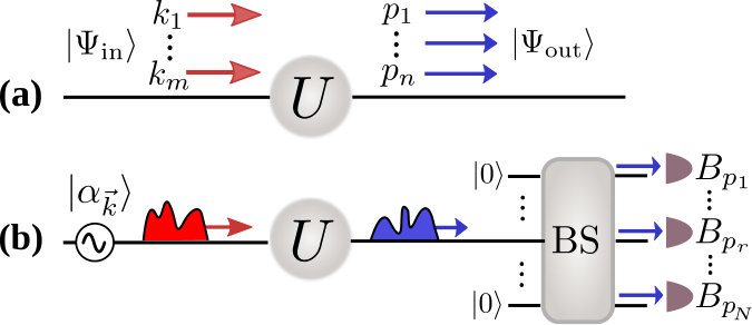 Figure 1
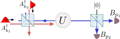 Figure 2
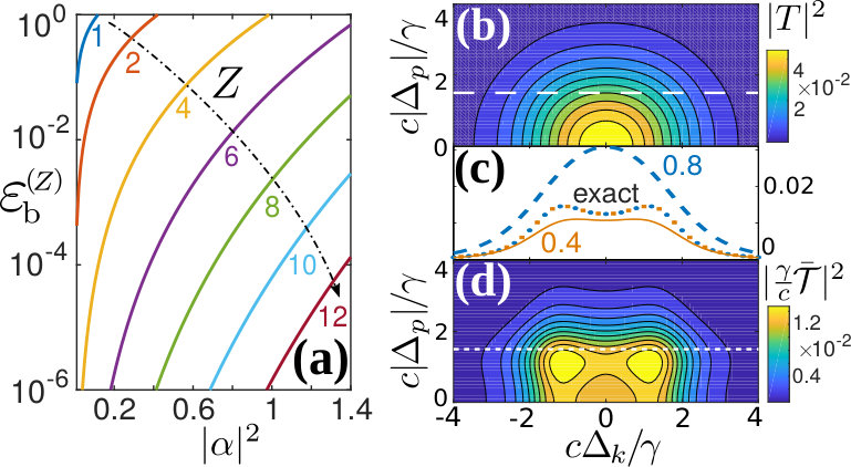 Figure 3
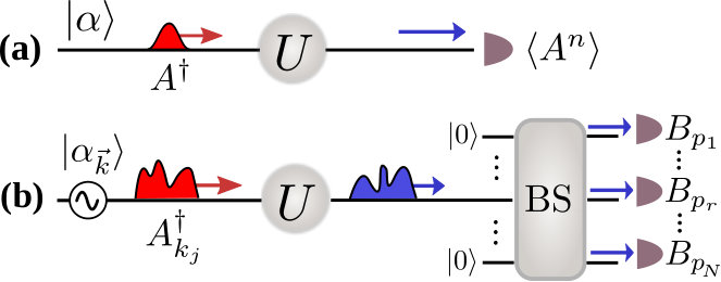 Figure 4
 Figure 5
Peer Reviews
No public reviews on file for this paper yet. If you reviewed it on a platform where reviews are public (OpenReview, ICLR, NeurIPS, ICML), you can paste yours below so the community can read it here.
Videos
No videos yet. Explain this paper in a talk, walkthrough, or lecture? Add one.
Taxonomy
TopicsAdvanced Optical Sensing Technologies · Random lasers and scattering media · Photoacoustic and Ultrasonic Imaging
Multiphoton Scattering Tomography with Coherent States
Tomás Ramos
Instituto de Física Fundamental IFF-CSIC, Calle Serrano 113b, Madrid 28006, Spain
Juan José García-Ripoll
Instituto de Física Fundamental IFF-CSIC, Calle Serrano 113b, Madrid 28006, Spain
Abstract
In this work we develop an experimental procedure to interrogate the single- and multiphoton scattering matrices of an unknown quantum system interacting with propagating photons. Our proposal requires coherent state laser or microwave inputs and homodyne detection at the scatterer’s output, and provides simultaneous information about multiple —elastic and inelastic— segments of the scattering matrix. The method is resilient to detector noise and its errors can be made arbitrarily small by combining experiments at various laser powers. Finally, we show that the tomography of scattering has to be performed using pulsed lasers to efficiently gather information about the nonlinear processes in the scatterer.
pacs:
03.65.Nk, 42.50.-p, 72.10.Fl
It is now possible to achieve strong and ultrastrong coupling between quantum emitters and propagating photons using superconducting qubits Astafiev et al. (2010); Hoi et al. (2011, 2013); Forn-Díaz et al. (2017), atoms Tiecke et al. (2014); Goban et al. (2015); Solano et al. (2017) or quantum dots Arcari et al. (2014) in photonic circuits, or even molecules in free space Hwang et al. (2009). This has motivated a stunning progress in the theory of single- and multiphoton scattering using wave functions Shen and Fan (2005) and the Bethe ansatz Shen and Fan (2007), as well as input-output theory Fan et al. (2010); Caneva et al. (2015), diagrammatic calculations Pletyukhov and Gritsev (2012); Laakso and Pletyukhov (2014); Hurst and Kok (2017), and path integral formalism Shi and Sun (2009); Shi et al. (2015). Very recently, the theory has even covered the ultrastrong coupling regime Shi et al. (2017). Experiments, however, cannot yet recover all the scattering information predicted by those studies, and are limited to comparing low-power coherent state transmission coefficients Astafiev et al. (2010); Forn-Díaz et al. (2017); Pechal et al. (2016), cross-Kerr phases Hoi et al. (2013), and antibunching Hoi et al. (2011). We therefore need an ambitious framework for reconstructing the complete one-, two-, or ideally any multiphoton scattering matrix. Such framework would allow studying the elastic Peropadre et al. (2013), and inelastic Goldstein et al. (2013) properties of quantum impurities in waveguides, quasi-particle spectroscopy Kurcz et al. (2014), interactions Gorshkov et al. (2010) in quantum simulators, and even characterizing all-optical quantum processors.
In this Letter we present a theoretical and experimental framework for estimating the scattering matrix
[TABLE]
which describes the transition amplitude from an input state of photons with generic quantum numbers , to an asymptotic output state of photons with labels [cf. Fig. 1a]. Operator represents the evolution in the limit of infinitely long time, and are generic input and output bosonic operators acting on the vacuum state . Our proposal assumes an experimental setup that injects coherent states and performs homodyne detection at the output of a generalized multiport beam splitter [cf. Fig. 1b]. Combining measurements with different input phases and amplitudes, we can approximate Eq. (1) with arbitrarily small error. The scheme is ideally suited for superconducting circuit and nanophotonic experiments, because all noise from amplifiers or detectors is canceled without previous calibration, similar to the dual-path method Menzel et al. (2010); Candia et al. (2014); da Silva et al. (2010).
In this Letter we also prove that the nonlinear contributions in the scattering are efficiently activated only for finite length input wave packets . However, standard deconvolution techniques applied to such experiments accurately and robustly reconstruct the scattering matrix in the monochromatic limit. We exemplify all these ideas for a two-level scatterer, whose scattering matrix is known Fan et al. (2010) and has only been probed at the single-photon level Astafiev et al. (2010); Hoi et al. (2011). This Letter is closed with a discussion on the generality of the protocol, and possible experimental implementations.
Scattering tomography protocol.–
Our presentation begins with the tomography architecture, continues with a discrete set of input states and a corresponding set of measurements, and closes with a general reconstruction formula for the scattering matrix. As shown in Fig. 1b, the setup consists of the quantum scatterer to be analyzed —or any active or passive optical medium—, a photonic channel that couples the light in and out of the scatterer, a signal generator to prepare the input states, and a multiport beam splitter that divides the output signal into independent measurement ports.
Our protocol requires a specific set of input states to probe the scatterer: coherent state wave packet inputs , created on top of the vacuum 111Throughout this work we assume that the scatterer has unique initial and final states, which are implicit in the definition of , but this restriction can be easily lifted. through a superposition of bosonic modes
[TABLE]
where are complex weights and the mean photon number 222The normalization of the coherent state (2) implies that the mean photon number is given by , where the commutators are not orthonormal for wave packets.. These multimode coherent states can be prepared using a signal generator [cf. Fig. 1b], or combining laser pulses through beam-splitters [cf. Fig. 2]. While later examples assume wave packets centered around momenta , the formalism allows to label any set of quantum numbers: frequency, polarization, path, etc.
The output of the scatterer is led through a balanced multiport beam splitter into homodyne detectors. At each output port, we filter outgoing photons with quantum numbers , and measure the quadratures to reconstruct the Fock operators . The nature of the beam splitter transformation is irrelevant, but all detectors should get a similar fraction of the scattered output, typically Combining the homodyne measurements we estimate any correlation function of the form
[TABLE]
where the filtered labels are to the outgoing indices in the scattering matrix sector to be estimated (1). Note that any set size is possible.
The expectation value (3) is an analytic function of the complex amplitudes . Each order of the Taylor expansion of is determined by a different sector of the scattering matrix. As explained in the Supplemental Material Sup , the values for different complex amplitudes —i.e. the correlation functions for different input states (2)—, can be added together, so as to cancel all terms except a desired sector of the scattering matrix and a small error. This is the basis for our protocols.
Protocol 1** (General)**
Let us assume a setup such as the one in Fig. 1b. In order to reconstruct the scattering matrix (1) with and , we will prepare input states , labeled by , and . The input states (2) built from wave packets only differ in the choice of phases
[TABLE]
For each input state, we measure the amplitudes repeatedly, gathering statistics to reconstruct all correlations , for . The scattering matrix is approximated as
[TABLE]
with a controlled error scaling as .
Note how the same set of measurements outcomes provides a simultaneous reconstruction of all scattering matrices from sizes up to .
Elastic scatterers.–
The reconstruction protocol simplifies when scattering conserves the total number of photons. This happens for emitters with one ground state and Jaynes-Cummings type interactions with symmetry (no cyclic transitions). The scattering matrix (1) is exactly zero for , quadrature measurements do not depend on global input phases and the total number of measurement setups reduces to .
Protocol 2** (Elastic scatterers)**
When it is a priori known that the scatterer conserves the photon number, we follow the steps in Protocol 1, but reduce the choice of input states to , where and
[TABLE]
with an error bounded by .
Examples.–
Experiments with superconducting or optical qubits at low power are well described by a RWA Hamiltonian Fan et al. (2010), and we can apply Protocol 2. For a single photon we require only one input with arbitrary, but small, complex amplitude , and the measurement of one quadrature , obtaining
[TABLE]
This formula includes the limit of state-of-the-art experiments Astafiev et al. (2010); Hoi et al. (2011); Forn-Díaz et al. (2017), where the transmission and reflection coefficients of single photons with momentum and fixed polarization, and , are recovered from the ratio between the input amplitude of a monochromatic coherent beam, and the scattered amplitude .
The reconstruction of the two-photon scattering matrix demands at least two measurement ports, and , and a set of two input modes, and . As shown in Fig. 2, an experiment could combine two independent pulses through a beam splitter, and then direct the scattering output to two homodyne measurement devices for estimating the correlations . For a RWA model, we reconstruct
[TABLE]
using only two different input phases. If we cannot ensure symmetry because of inelastic channels Goldstein et al. (2013), ultrastrong coupling Shi et al. (2017), external driving on the scatterer Bishop et al. (2009), etc., we need 8 input states with varying global phase , and the general reconstruction formula (5). However, the same measurements provide us with estimates for , , , and .
Arbitrary reconstruction error.–
There are four sources of error in our reconstruction protocol: (i) quantum fluctuations in quadrature measurements, (ii) detector noise, (iii) imperfect input preparation, and (iv) approximation error. The first source of error scales as and can be decreased arbitrarily by increasing the number of repetitions of the experiment. By design, our protocol is intrinsically resilient to the second source of errors, because detector noise averages out when combining odd powers of quadratures from different detectors —similar to Refs. Menzel et al. (2010); Candia et al. (2014); da Silva et al. (2010).
Imperfections in the preparation of relative phases , laser power , and global phases , add linear contributions to the error, , and Sup . These errors can be controlled using standard calibration and phase stability techniques, and ensuring to work at moderate powers, .
Indeed, a feature of our method is that we are not restricted to working at infinitesimal . Instead, we can combine different estimates of the scattering matrix, , reconstructed from Eqs. (5)-(8) at different laser powers , to create a refined estimate with a higher order truncation error . The simplest instance of this idea requires one extra estimate
[TABLE]
at a larger power , to give . Higher order formulas can be derived analytically Sup , with error estimates that are strongly suppressed and allow working at . This is illustrated by Fig. 3a, where we plot an upper bound for for elastic two-photon scattering, as a function of the smallest laser power , for different approximation orders . For , we just need and , to get error bounds , showing the potential of this method to estimate multiphoton scattering matrices.
The need of wave packets.–
We will now discuss the case in which describes the momentum degree of freedom. We will argue that our reconstruction protocol requires input states that are finite length wave packets
[TABLE]
built from normalized superpositions of plane waves , with and . The discussion below does not include other discrete degrees of freedom, which can be straightforwardly added Sup .
The use of pulsed light contrasts with existing theory, which computes the scattering matrix elements for well defined momentum modes Fan et al. (2010); Caneva et al. (2015); Shi et al. (2015), as in
[TABLE]
The reasons for studying the monochromatic are (i) the possibility of analytical calculations and that (ii) it reveals the underlying nonlinearity of the scatterer. Take, for instance, the two-photon scattering matrix for a two-level system, which can be decomposed as Fan et al. (2010); Xu et al. (2013)
[TABLE]
with the photon dispersion relation and the velocity of light. The first two terms in Eq. (The need of wave packets.–) connect independent single-photon events , while the last one is the nonlinear contribution that describes photon-photon interaction mediated by simultaneous interaction with the scatterer, such as the two-photon Kerr effect Hoi et al. (2013).
Interestingly, and are related through an integral,
[TABLE]
We will evaluate this for the two-photon scattering matrix in a tomography experiment using Gaussian pulses , with
[TABLE]
We are specially interested in analyzing how the nonlinearity manifests in the monochromatic limit of negligible bandwidth . To do so, we focus on forward scattering in a waveguide with linear dispersion relation , but this is easily extended Sup . The main result is that the measured two-photon scattering matrix also splits into single- and two-photon contributions, which are given by the convolutions,
[TABLE]
The transmission coefficient appears in Eq. (17) as a consequence of energy conservation, , as well as the relation for the integration momenta in Eq. (18). Because the kernel in Eq. (18) is a product of three Gaussians Sup and is typically a smooth and bounded function, any nonlinear contribution to the scattering experiment vanishes as we make the wave packet width tend to zero,
[TABLE]
This argument can be extended to higher order processes, 333This derives from Eq. (15) by a purely dimensional analysis, assuming , and a monochromatic nonlinear contribution that satisfies energy conservation as in Eq. (The need of wave packets.–)., illustrating the fact that nonlinear terms can only be activated when photons coexist in the scatterer, and the probability of this overlap tends to zero as the wave packet length tends to infinity. We, therefore, conclude that an efficient reconstruction of the full scattering matrix for two or more photons requires working with finite duration wave packets.
Deconvolution formulas.–
Even if we need wave packets to get an experimentally measurable signal, we can still reconstruct the monochromatic properties from such experiments using standard deconvolution techniques Ulmer and Kaissl (2003). We illustrate this by deriving the single- and two-photon forward scattering coefficients and from the measured and . This requires inverting Eqs. (17)-(18), which can be done analytically for Gaussian wave packets Ulmer and Kaissl (2003); Ulmer (2010); Fang et al. (1994). For the single-photon transmission we obtain,
[TABLE]
The inverse kernel contains Hermite polynomials and produces a convergent series provided the function to deconvolve is integrable Ulmer and Kaissl (2003); Ulmer (2010). As discussed above, the single-photon reconstruction still works with monochromatic beams, recovering the state-of-the-art experimental formula .
The reconstruction of the two-photon scattering strength from the measured values of involves a three-dimensional deconvolution using a product of the same inverse kernels Ulmer (2010). Energy conservation imposes that the only nonzero elements of have to be functions of the conserved average momentum , and the relative differences, and . For these elements we get,
[TABLE]
As an illustration, we evaluate the measured scattering matrix and the reconstructed monochromatic version , for a gedanken experiment with Gaussian pulses and a two-level scatterer. This problem admits an analytical solution Shen and Fan (2007); Fan et al. (2010); Sup with which we can test the reconstruction formulas (18) and (Deconvolution formulas.–). As shown in Figs. 3b and 3d, the measured matrix is broader than the monochromatic , due to the convolution with the Gaussians. However, we have found that provided the wave packet size remains on order of the scatterer linewidth , we can efficiently reconstruct from . We exemplify this in Fig. 3c, where we show how cross sections of obtained for two different widths (brown) and (blue) both reconstruct the exact result for after the deconvolution (brown and blue dots). The fact that is a good compromise should not be a surprise, as this is the regime which maximizes the nonlinear effects and the coexistence of photons. In general, the gaussian deconvolution with kernel (20) allows us to efficiently reconstruct any smooth sector of the scattering matrix, provided the measured function to deconvolve is integrable Ulmer and Kaissl (2003); Ulmer (2010) and the order of the width is chosen according to the ‘bandwidth’ of the specific scatterer.
Summary and outlook.–
This Letter introduced a tomography protocol for reconstructing the scattering matrix of a photonic field interacting with a quantum scatterer, using coherent states and correlated homodyne measurements. We have demonstrated that pulsed spectroscopy is needed to gather information about the nonlinear processes in scattering. This could remind the reader of two-dimensional pulsed spectroscopy methods in the optical and NMR realms Keusters et al. (1999); Cho (2008), but those constitute a time-resolved interrogation of the scatterer, whereas our protocol studies the asymptotic transformation (1) imparted by an optical medium in a propagating field.
While our protocol is inspired by recent progress in the fields of waveguide QED and nanophotonics, the idea, setup, and formulas can be used to probe any system that is in contact with a linear bosonic field. This includes not only superconducting qubits in strong-coupling Astafiev et al. (2010); Hoi et al. (2013) or ultrastrong-coupling 1D setups Forn-Díaz et al. (2017), but also studying single molecule emitters in three dimensions Hwang et al. (2009), or other extended optical media. The reconstruction protocol is so general that it does not require any a-priori knowledge of the quantum emitter, and can be applied in the presence of decoherence and dissipation. We believe that under such circumstances our protocol is optimal, but particular symmetries or a better understanding of the models can lead to substantial simplifications to be considered in future work.
Acknowledgements.
The authors acknowledge support from the MINECO/FEDER Project FIS2015-70856-P and CAM PRICYT Research Network QUITEMAD+ S2013/ICE-2801.
Contents
- •
I.—Derivation of the general scattering tomography relations.
- •
II.—Arbitrary reconstruction error by combining multiple estimates of the scattering matrix.
- •
III.—Deconvolution with gaussian wave packets in dispersive channels.
- •
IV.—Imperfections in the input state preparation.
I I. Scattering tomography relations
In this section, we derive the central relations underlying our multiphoton scattering tomography protocol. We relate the components of an unknown unitary matrix with the measurement of certain photonic quadrature correlations at the output, when probing the system with coherent state inputs (see Fig. 4). In a first order approximation, a small reconstruction error requires attenuated coherent state inputs, but this restriction is lifted in Sec. II by combining various estimates at different input powers.
The derivation is split into two parts. First, in Sec. I.A, we show how to reconstruct the scattering matrix elements in the total photon number basis, namely
[TABLE]
These matrix elements describe processes involving incoming and outgoing photons, without resolving other photonic degrees of freedom. Then, in Sec. I.B, we extend the protocol to identify photons by a generic quantum number , which accounts for any combination of external and/or internal photonic properties such as momentum, frequency, polarization, etc. In particular, we can reconstruct general scattering matrix elements of the form,
[TABLE]
describing processes from incoming photons with general quantum numbers to outgoing with . As explained below, the injection and detection of photons with specific quantum numbers requires the use of a signal generator at the laser input and a multiport beam splitter at the measurement output (see also Fig. 4b).
I.1 A. Tomography of a scattering matrix in the photon number basis
We start by considering the situation sketched in Fig. 4a, where photons propagate along a one-dimensional (1D) channel and interact with an unknown quantum medium according to a scattering matrix . As a result, any photonic input state is transformed into the output , with the only restriction that the vacuum state remains invariant, i. e. . Besides this last condition, the unitary is completely arbitrary, and we show in the following how to reconstruct its elements using homodyne detection.
First, our scattering tomography protocol requires the preparation of a coherent state input,
[TABLE]
where is a bosonic creation operator of a photon in the channel, satisfying , and is the complex vacuum displacement with module and phase .
Secondly, we require the measurement of photon output correlations of the form
[TABLE]
which can be determined to any order by measuring the output quadratures and via homodyne detection, with .
To derive the relation between the scattering matrix elements (22) and the correlations (25), let us first consider the measurement of a general operator at the output, namely . If we replace here the definition of the coherent state (24) and decompose in terms of its module and phase, we obtain
[TABLE]
where the coefficients read,
[TABLE]
In addition, can only take two values: in the special case (since then ), and in any other case. In particular, for the choice we can simply take , but we keep the derivation general.
Our aim now is to solve for the coefficients of the form from Eq. (26), since they correspond to the scattering matrix elements (22) when . As we show in the following, we can isolate the coefficients , for , by preparing different coherent input states of the form (24), and measuring for each of them (). Importantly, we choose the different coherent state inputs to have the same module , but different global phase as . As a result, we can replace and in Eq. (26), obtaining a set of independent equations for the unknowns , which read
[TABLE]
To see how to choose the phases in order to solve for the coefficients in Eq. (28), let us multiply Eq. (28) by and sum over all values , obtaining the equation,
[TABLE]
after the convenient change of variables, and . We have defined the new coefficients,
[TABLE]
and the sum over , denoted with a bold sum symbol , corresponds to a sum where goes from to in steps of . Choosing the phases as
[TABLE]
we see that the last factor on the right hand side of Eq. (29) becomes the discrete Fourier transform of a periodic Kronecker delta,
[TABLE]
with taking any integer value due to the function periodicity of size . When replacing (32) into Eq. (29), we see that all non-vanishing terms must satisfy , with and of the same parity as . This allows us to select specific terms in the sum. In particular, if we set
[TABLE]
then all non-zero terms with in Eq. (29) can only take or equivalently , as they all lie within the first period of the delta function. In addition, since is bounded by , then all terms with vanish, and our target coefficients appear to lowest non-zero order , for , namely
[TABLE]
Here, the bounds of are given by and where the function rounds the number to its nearest smaller integer. From Eq. (34) it is clear that in the case of attenuated coherent state inputs, , all terms on order or higher are further suppressed and we can solve for with a small relative error. By formally solving for the coefficient in Eq. (34), we obtain the main result of this subsection,
[TABLE]
which relates the desired matrix elements , for powers , with the measurements at the output. In particular, when replacing in Eq. (35), we access all the scattering matrix elements in Eq. (22), describing incident photons to any number of outgoing photons in the channel . As , we can take and the number of measurements needed is .
Regarding the error , we find a precise expression for it in terms of a series with even powers of the coherent state amplitude as,
[TABLE]
From here it is clear that scales as in the case of attenuated coherent states. The coefficients are independent of the coherent input power, and are given in general by,
[TABLE]
In addition, using Eqs. (27), (36) and (37), as well as the triangular inequality, we can show that the error (36) is strictly bounded by , where the bound for the coefficients reads
[TABLE]
and are the photon number states.
It is worth highlighting the special case where we a priori know that the number of photons is conserved during the scattering, i. e. , since then the tomography protocol is strongly simplified. In particular, only the diagonal components are nonzero and a single measurement, , is enough to determine them. To see this, notice that the conservation of photon number and implies that is only nonzero for . Using this in Eq. (29) allows us to derive the same Eqs. (34) and (35), but now valid for and all , since in this case all coefficients appearing at lower order than are zero regardless the value of . Another peculiarity of this elastic scattering case is that the bound for the error in Eq. (38) takes a very simple closed form. Again, using and the conservation of photon number, we can set and in Eq. (38), and additionally using , we find a simple bound for the coefficients in this elastic case,
[TABLE]
As a result, the error in Eq. (36) is strictly bounded by a displaced exponential for all , namely
[TABLE]
I.2 B. Tomography of a scattering matrix with resolution on photon degrees of freedom
In this subsection, we extend the protocol to measure scattering matrix elements with resolution on a generic quantum number , describing any combination of external or internal photon degrees of freedom as in Eq. (23). First, in Sec. I.B.1. , we generalize Eq. (35) to determine matrix elements of the form , which describe input states of photons with different generic quantum numbers . Then, in Sec. I.B.2. , we give details on a beam splitter setup to measure the output quadrature correlations (see Fig. 4b), and we show how to reconstruct the general scattering matrix elements (23) from these correlations.
I.2.1 1. Multimode coherent state input
First, we need a mechanism to inject photons, with various values of a combined quantum number , at the input of the scatterer (see Fig. 4b). To this end we prepare a coherent state input as in Eq. (24), but now for a multimode superposition , defined for different components as
[TABLE]
Here, for , are the creation operators of a photon with generic quantum number , and is a projection vector normalized as , such that . Notice that the modes do not satisfy standard commutation relations in general, allowing us to describe photon wave packets as inputs. For instance, for Gaussian wave packet modes as defined in Eqs. (12) and (16) of the main text, we obtain .
The coherent state input corresponding to the multimode superposition (41) can be expressed more explicitly as
[TABLE]
where the weights on each component are given by , with , and the mean photon number reads . This multimode coherent state can be prepared using a signal generator (see Fig. 4b), which is readily implemented in microwave and optical photonic setups.
When we vary the global phase of the displacement weights as , with and defined in the previous subsection, we can apply the result (35) to the multimode superposition operator in Eq. (41), and thereby determine the matrix elements , with the associated error . However, this is not enough the determine matrix elements of the form , since when expanding the multinomial in , we see that it contains many unwanted terms, namely
[TABLE]
Notice that the sums over are constrained to values that satisfy , as demanded by the multinomial theorem.
Our aim in this subsection is therefore to extract from the above relation the term and relate it to by canceling all unwanted terms. We achieve this by performing additional measurements as in the previous subsection, but now we vary the relative phases in the multimode superposition as . Here, for denote the different values that the phase of each component can take, and we keep all the moduli fixed. We also use the shorthand notation, , to arrange the values of the different indices. To see how to choose the phases in order to cancel the unwanted terms in Eq. (44), we divide this equation by and sum over all independent values of , for , and , obtaining
[TABLE]
Choosing , for all , we can use the same property (32) as in the previous subsection and form periodic Kronecker deltas in Eq. (45),
[TABLE]
with and arbitrary integers. Importantly, due to the constrains and , it is enough to choose as
[TABLE]
so that the deltas in Eq. (45) cancel all terms, except for the one with and , and we obtain the desired relation,
[TABLE]
With the choice (47), we see that the relative phases take the simple values and , resulting only in sign changes of the vector components as, and . Therefore, from now on (and also in the main text), we conveniently redefine the indices as
[TABLE]
such that the different values of vector components are simply given by
[TABLE]
Finally, replacing the result (35) into Eq. (48), we obtain a closed relation for the matrix elements , with , and the various measurements , given by
[TABLE]
Here, we have used the new notation (49) for , and defined the weights of the coherent states in Eq. (43) as
[TABLE]
with , and as previously defined in Eqs. (31) and (33).
The error in Eq. (51) is also of the form,
[TABLE]
where the modified error coefficients are given by
[TABLE]
with , defined in Eq. (37), now depends on via in the coefficients (27).
I.2.2 2. Homodyne detection at beam splitter outputs
Notice that Eq. (51) directly gives the desired scattering matrix elements,
[TABLE]
in the case we replace . Using the resulting relation, however, demands the measurement of specific correlation functions at the scatterer’s output on channel , namely
[TABLE]
To distinguish the contribution of photons with different generic quantum numbers in the above correlations (56), a filtering mechanism at the scatterer’s output is needed. Therefore, we connect the output of the scatterer to a multiport beam splitter, which divides the scattered signal into independent channels (see Fig. 4b). At each independent output port of the beam splitter, labeled by , we measure the quadratures and , and reconstruct the field operator for outgoing photons with quantum number . When gathering enough statistics via homodyne detection, we can determine the correlations,
[TABLE]
which can be related to the correlations in Eq. (56) via the beam splitter transformation .
Notice that the specific form of the beam splitter transformation is irrelevant, as long as each output port gets a similar fraction of the scattered signal and that all other input ports are in vacuum (see Fig. 4). As a practical example, let us consider the transformation for a balanced multiport beam splitter, for which the photonic amplitude operators at each independent output, , read
[TABLE]
Here, with denote the annihilation operators on the vacuum input ports different than channel . As these extra channels are independent between each other and with channel , they satisfy the commutation relations, , and , implying .
Using expression (58) in Eq. (57), we see that the required correlations (56) can be accessed by measuring at the outputs of the beam splitter. In fact, both correlations are just proportional to each other:
[TABLE]
Finally, we just replace into Eq. (51) and use the relation (59) to obtain the general scattering matrix elements in terms of the measurable correlations , as
[TABLE]
This is the main result of the paper and is shown in Eqs. (5) and (8) of the main text, for the general () and elastic () cases, respectively.
The truncation error appearing in the final result (60) has a closed analytical upper bound in the case that the scattering matrix conserves the number of photons (Protocol 2 of the main text). From Eqs. (53)-(54) we see that this problem is equivalent to find a closed bound for the coefficients . Therefore, we replace in Eq. (38) and use Eq. (58), to re-express the bound in terms of the operators as
[TABLE]
Since conserves the total number of photons, we can set and in Eq. (61), and additionally using the Cauchy-Schwarz inequality, we obtain
[TABLE]
The next step is to decompose the total number state into components along all channels of the interferometer, and using the fact the the sum of photons in all channels is fixed, , we can bound the numerator in Eq. (62) by . Using this result in Eq. (62) we obtain a simple bound for the coefficients similar to Eq. (39) as , and replacing this into Eq. (54), we find the bound for the coefficients as well,
[TABLE]
For simplicity, let us consider the case that we prepare the multimode coherent state inputs with equal projections, . The normalization condition, stated below Eq. (43), implies , in the case of gaussian wave-packets as in the main text. Using this and , we find a strict bound for the coefficients that is easy to evaluate,
[TABLE]
and replacing this into Eq. (53), the strict bound for the error reads,
[TABLE]
II II. Arbitrary reconstruction error by combining multiple estimates
An intrinsic error that limits the precision of our tomography protocol is the reconstruction error . In this section, we show how to reduce this error by performing the scattering tomography protocol in Eq. (60) at different laser powers and combining the outcomes in a clever way. Importantly, this allows us to perform the tomography at non-perturbative mean photon numbers , lifting the requirement of attenuated coherent state inputs.
A first order estimate of the scattering matrix is given by the outcome of our protocol in Eq. (60) as,
[TABLE]
with an error , scaling as . Interestingly, if we consider another first order estimate measured at a larger power , with , we can combine it with , and cancel the error term of order . As a result, we obtain a second order estimate,
[TABLE]
with a higher order approximation error,
[TABLE]
that scales as . Here, the modified error coefficients read . This process can be iterated up to arbitrary order using the recursion relation,
[TABLE]
which gives the estimate of order from two estimates of a lower order: and . In general, a -order estimate has an error given by
[TABLE]
where the -order coefficients can expressed in terms of in Eq. (54) as
[TABLE]
The final step is to express a general -order estimate in terms of first order estimates only, as these are the ones that we measure in practice via (66). Using times the recursion relation (69), it is straightforward to check that can always be expressed as a linear combination of different first order estimates , measured at increasing laser powers , with and , as
[TABLE]
Here, the coefficients are determined recursively from Eqs. (67) and (69). As an example, for , the coefficients are explicitly given by
[TABLE]
In summary, the elements of the scattering matrix can be estimated with a -order error given in Eqs. (70)-(71) by combining first order estimates (66), obtained at incresing laser powers as
[TABLE]
Importantly, the -order error is strongly suppressed by its prefactor, which allows one to perform the scattering tomography protocol at non-perturbative laser powers . We show this explicitly by numerically evaluating the upper bound of the -order error in the case of elastic scattering , which is obtained from Eqs. (65), (70), and (71) as
[TABLE]
In Fig. 5a-b, we plot in logarithmic scale, as a function of the minimal mean photon number and the number of estimates , for for two values of the factor . For , we indeed get a good error bound of for and a moderate number of estimates . Figure 3a of the main text shows the same bound and the same parameters, but evaluated in the specific case .
In general, the error suppression is stronger for smaller , as it becomes clear by comparing Figs. 5a and 5b. Experimentally, the value of this factor is restricted by the precision to increase the laser power as . Finally, notice that for a given starting mean photon number and a fixed value of the factor, there will be an optimal number of estimates that gives the maximum supression of the error. For higher than the optimal, the error will actually increase due to its prefactors (see Fig. 5b).
III III. Deconvolution with gaussian wave packets in dispersive channels
To be sensitive to nonlinear multiphoton scattering events, our scattering protocol requires wave packet input modes in the case the quantum number describes a continuous degree of freedom such as momentum or frequency. Therefore, in the following analysis we want to distinguish between continuous and discrete photon degrees of freedom, which we label by and , respectively. For instance, photon polarization and/or path can be included in the quantum numbers. Using this separation of labels, we assume that the generic bosonic modes in Eq. (43) are prepared as
[TABLE]
where is the square-normalized wave packet profile for the continuous variable , centered at , and describe monochromatic photons with quantum numbers and , satisfying standard communation relations .
The choice of input modes in Eq. (79) implies that our scattering protocol gives us direct access to the ‘wave packet’ scattering matrix elements only, given in general by
[TABLE]
As explained in the main text, the scattering matrix elements in the monochromatic Fock basis, , can still be accessed by using Eq. (79) and inverting the integral relation,
[TABLE]
Therefore, one needs to perform a deconvolution on the continuous variables for each combination of the discrete variables , which in turn requires the measurement of the wave packet matrix elements for all convinations of quantum numbers . As we are mainly interested in illustrating how to perform a single deconvolution, in the remainder of the section, as well as in the main text, we assume that all discrete quantum numbers are equal and we absorb them in the definition of the photon operators and . This simplifies the equations considerably, and we just have to keep in mind that to describe additional internal degrees of freedom of photons, we have to repeat the same deconvolution procedure for each combination of of the discrete labels .
In this section, we show how to analytically solve the deconvolution integral for the monochromatic single- and two-photon scattering matrices in Eq. (The need of wave packets.–) of the main text, which corresponds to the more general Eq. (III) in the case the continuous degree of freedom corresponds to momentum or frequency, and all photons have the same discrete degrees of freedom. To do so, we assume wave-packets with gaussian shape and a possibly dispersive photonic channel, as shown below.
In Sec. III.C, we show the analytical expressions for the single- and two-photon scattering matrices used in Figs. 3(b)-(d) of the main text to test the gaussian deconvolution formulas.
III.1 A. Gaussian deconvolution in a dispersive channel
As we want to discuss photons in a dispersive channel, the deconvolution integrals turn out to be simpler when working with frequency modes instead of momentum. Therefore, in this subsection we derive all deconvolution formulas in terms of frequency-direction modes, and in the next subsection we map the results to momentum, connecting to the specific formulas shown in the main text.
In the special case that the dispersion relation is symmetric, , and the group velocity is antisymmetric, , the propagating momentum modes can be unambiguously related to frequency-direction modes , as
[TABLE]
Here, the mapping assumes that photons with propagate to the right (), while photons with propagate to the left (), and we identify these directions with the quantum number . In addition, the frequency of the photons has a one-to-one correspondence with the wavenumber via the invertible function . Note that this relation (82) is not valid for , since the group velocity necessarily vanishes . Nevertheless, we will always consider propagating wave packets (79) with negligible components on this mode.
The wave packet operators in Eq. (79) can be expressed in terms of frequency-direction modes as
[TABLE]
where the corresponding wave packet profile is related to its momentum counterpart by
[TABLE]
In particular, we choose wave packets with a gaussian profile defined as
[TABLE]
such that the wave packet mode is built exclusively from monochromatic frequency modes propagating in the same direction . We also assume that the central frequency of the wave packet is much larger than its width, , to ensure a vanishing component on the non-propagating mode .
Using all these considerations, we can re-express the general integral equation (15) of the main text, in terms of frequency-direction modes, as
[TABLE]
where denote the monochromatic scattering elements from incoming photons with frequencies , and directions , to outgoing ones with frequencies , and directions , respectively.
In the following, we specialize the discussion to the single- and two-photon matrix elements of a scatterer with a single ground state. In this case, the conservation of energy allows us to decompose the monochromatic scattering components as in Eq. (The need of wave packets.–) of the main text:
[TABLE]
Here, contain the reflection and transmission coefficients, and the nonlinear contribution describes photon-photon interactions mediated by the scatterer.
Using Eqs. (88)-(89) in Eq. (87), simplifies the integral relations by reducing their dimensionality. In particular, the single-photon scattering matrix satisfies,
[TABLE]
On the other hand, the two-photon ‘wave packet’ scattering matrix can be also decomposed into linear and nonlinear contributions,
[TABLE]
where the non-linear part reads,
[TABLE]
Here, the kernel is the product of three Gaussians,
[TABLE]
and we conveniently defined the new variables , and , , and .
Interestingly, both Eqs. (90) and (92) can be analytically inverted as they involve a product of Gaussian kernels for independent integration variables. Therefore, following Refs. Ulmer and Kaissl (2003); Ulmer (2010); Fang et al. (1994) of the main text, we obtain
[TABLE]
where the inverse Gaussian kernel is given by
[TABLE]
Here, are Hermite polynomials and the series is convergent because and decay exponentially fast.
These last Eqs. (94)-(95) are direct analytical relations for the single- and two-photon scattering coefficients in terms of the ‘wave packet’ counterparts, measurable with our tomography protocol. Moreover, they are valid for any dispersive photonic channel, satisfying and . In the next subsection, we connect to the expressions stated in the main text, by transforming to momentum variables, and specializing to a linear dispersion relation .
III.2 B. Gaussian deconvolution in momentum modes for a non-dispersive channel
The monochromatic scattering elements in momentum and frequency basis can be related using Eq. (82) as
[TABLE]
where we used the identifications, , , , and . In addition, using the explicit formulas (88)-(89), we obtain the same formulas for the momentum monochromatic elements in the main text,
[TABLE]
but now with the coefficients given for dispersive media as,
[TABLE]
The wave packet profile used in Eq. (86) to perform the deconvolutions, can be recast in momentum as
[TABLE]
where the is the momentum width used in the main text.
Finally, when evaluating the above expressions for a linear dispersion relation and forward scattering , as in the main text. In particular, the wave packet profile reduces simply to and the scattering coefficients read,
[TABLE]
where , , and .
III.3 C. One- and two-photon scattering matrix for a qubit weakly coupled to a 1D waveguide
In this subsection, we explicitly state the results shown in Refs. Shen and Fan (2007); Fan et al. (2010) of the main text, for the one- and two-photon scattering matrices of a two-level system weakly coupled to a 1D photonic waveguide. We use these analytical results in Figs. 3(b)-(d) of the main text to test the deconvolution formulas shown above. In particular, the monochromatic single-photon scattering matrix has the form of Eq. (88) with the reflection and transmission coefficients given by
[TABLE]
Here is the transition frequency of the two-level system and its decay rate. The two-photon scattering matrix is of the form of Eq. (89), with the two-photon interaction strength given by
[TABLE]
This is the nonlinearity we replace in Eq. (18) of the main text (with the proper change of variables as explained in the previous subsections) to evaluate the prediction for a scattering experiment with gaussian wave packets and a weakly coupled qubit. We then perform a deconvolution of the result using Eq. (Deconvolution formulas.–) of the main text, and check that the result agrees with the initial Eq. (107), which allows us to test the deconvolution formulas.
IV IV. Imperfections in the input state preparation
In this section we discuss errors in the reconstruction of the scattering matrix elements, which are caused by imperfections in the preparation of the coherent state inputs. The analysis includes deviations in the relative phases [cf. Sec. IV.A], laser power [cf. Sec. IV.B], and global phases [cf. Sec. IV.C].
IV.1 A. Deviations in relative phases
In the case the scatterer conserves the photon number, we can apply Protocol 2 of the main text, and therefore the preparation of the various input states requires only the control of relative phases , for . If we go back to Eq. (48) in the derivation of the protocol and assume a small deviation, , in the ideal relative phases, we obtain the relation,
[TABLE]
where the ‘sign’ error is given to first order in the small deviations as
[TABLE]
with he average deviation .
The rest of the derivation for the reconstruction formula is the same as in Sec. I.B. In particular, when replacing Eq. (35) into the imperfect relation (108), we obtain the usual estimate of the scattering matrix in Eqs. (51) and (66), but now with the extra ’sign’ error given above,
[TABLE]
Notice that this small error in the relative phases is linear in the deviations, and thus can be controlled provided . Since does not depend on the laser power , the formula for the -order estimate is straightforwardly derived by reapeating the procedure in Sec. II., obtaining simply
[TABLE]
with and as given in Eqs. (72) and (70).
IV.2 B. Imperfections in laser power input
In the case there are imperfections in setting the mean photon number of the input states, , the procedure in Sec. II for combining estimates at well defined laser powers, , will be affected by an error as well. For a first order estimate, this error appears as
[TABLE]
Using the above expression in the procedure of Sec. II to combine estimates, we generalize Eq. (111),
[TABLE]
with the extra error due to imperfections in the laser power, given by
[TABLE]
Notice that for this error is also linear in the deviations,
[TABLE]
and it is small since high order terms in the sum (with ) are strongly suppressed by the coefficients in Eq. (71).
IV.3 C. Deviations in global phases
In this last section we discuss errors due to deviations in the global phase of the input states, , for . This is needed in the case that we do not know a priori if the scatterer conserves the photon number, and we have to apply the general Protocol 1 of the main text. If we go back to Eq. (35) in the derivation of the protocol (with ), the deviations will add an extra error to this expression, obtaining
[TABLE]
In addition to the usual approximation error , the error due to imperfect global phases reads,
[TABLE]
Including the error due to imperfect relative phases, we replace Eq. (117) into Eq. (108), and following the usual derivation, we obtain a more general expression for the first order estimate of ,
[TABLE]
Here, and are the approximation and sign errors already discussed, and the first order error due to imperfections in the global phases reads
[TABLE]
Additionally, if we now include the error due to imperfections in the laser power as in Eq. (114), with , and combine estimates as in Sec. II, we derive the most general -order estimate for ,
[TABLE]
with the -order error due to imperfect global phases given by
[TABLE]
Here, only the few first terms in the expansion contribute to the error as in strongly suppresses higher order terms with . Finally, notice that if we use moderate laser powers and assume small deviations in the global phases , the resulting error is small and linear in the deviations, scaling approximately as .
The reference list from the paper itself. Each links out to its DOI / PubMed record.
- 1Astafiev et al. (2010) O. Astafiev, A. M. Zagoskin, A. A. Abdumalikov, Y. A. Pashkin, T. Yamamoto, K. Inomata, Y. Nakamura, and J. S. Tsai, Science 327 , 840 (2010) . · doi ↗
- 2Hoi et al. (2011) I.-C. Hoi, C. M. Wilson, G. Johansson, T. Palomaki, B. Peropadre, and P. Delsing, Phys. Rev. Lett. 107 , 073601 (2011) . · doi ↗
- 3Hoi et al. (2013) I.-C. Hoi, A. F. Kockum, T. Palomaki, T. M. Stace, B. Fan, L. Tornberg, S. R. Sathyamoorthy, G. Johansson, P. Delsing, and C. M. Wilson, Phys. Rev. Lett. 111 , 053601 (2013) . · doi ↗
- 4Forn-Díaz et al. (2017) P. Forn-Díaz, J. J. García-Ripoll, B. Peropadre, J.-L. Orgiazzi, M. A. Yurtalan, R. Belyansky, C. M. Wilson, and A. Lupascu, Nature Phys. 13 , 39 (2017) . · doi ↗
- 5Tiecke et al. (2014) T. G. Tiecke, J. D. Thompson, N. P. de Leon, L. R. Liu, V. Vuletić, and M. D. Lukin, Nature 508 , 241 (2014) . · doi ↗
- 6Goban et al. (2015) A. Goban, C.-L. Hung, J. D. Hood, S.-P. Yu, J. A. Muniz, O. Painter, and H. J. Kimble, Phys. Rev. Lett. 115 , 063601 (2015) . · doi ↗
- 7Solano et al. (2017) P. Solano, P. Barberis-Blostein, F. K. Fatemi, L. A. Orozco, and S. L. Rolston, ar Xiv:1704.07486 (2017) .
- 8Arcari et al. (2014) M. Arcari, I. Söllner, A. Javadi, S. Lindskov Hansen, S. Mahmoodian, J. Liu, H. Thyrrestrup, E. H. Lee, J. D. Song, S. Stobbe, and P. Lodahl, Phys. Rev. Lett. 113 , 093603 (2014) . · doi ↗