Landau levels in QCD
F. Bruckmann, G. Endrodi, M. Giordano, S. D. Katz, T. G. Kovacs, F., Pittler, J. Wellnhofer

TL;DR
This study provides the first lattice simulation evidence of Landau level structures in Dirac eigenmodes within full QCD under magnetic fields, revealing how these levels influence quark observables.
Contribution
It introduces a novel lattice approach to identify and analyze Landau levels in four-dimensional QCD, connecting topological arguments with fermionic observable evaluations.
Findings
Identification of lowest Landau level modes in lattice QCD
Quantification of the lowest Landau level's contribution to quark condensate and spin polarization
Potential for comparison with low-energy QCD models using Landau level approximation
Abstract
We present first evidence for the Landau level structure of Dirac eigenmodes in full QCD for nonzero background magnetic fields, based on first principles lattice simulations using staggered quarks. Our approach involves the identification of the lowest Landau level modes in two dimensions, where topological arguments ensure a clear separation of these modes from energetically higher states, and an expansion of the full four-dimensional modes in the basis of these two-dimensional states. We evaluate various fermionic observables including the quark condensate and the spin polarization in this basis to find how much the lowest Landau level contributes to them. The results allow for a deeper insight into the dynamics of quarks and gluons in background magnetic fields and may be directly compared to low-energy models of QCD employing the lowest Landau level approximation.
Click any figure to enlarge with its caption.
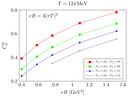 Figure 1
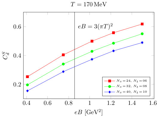 Figure 2
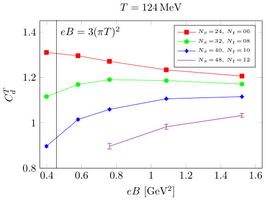 Figure 3
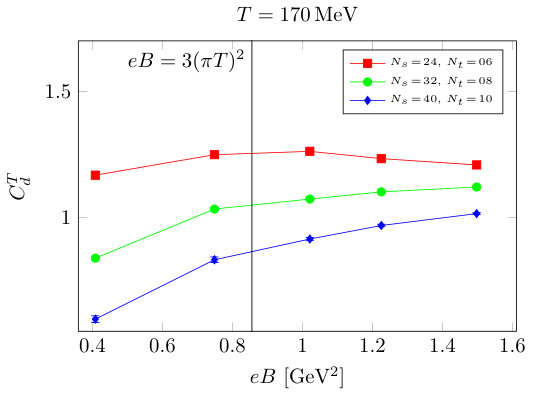 Figure 4
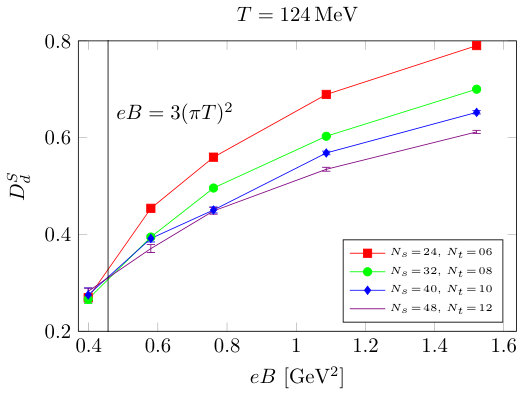 Figure 5
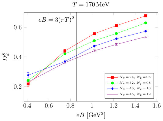 Figure 6
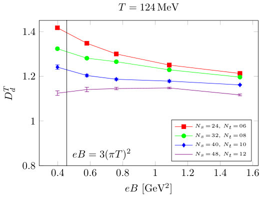 Figure 7
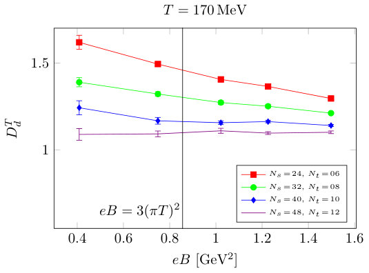 Figure 8
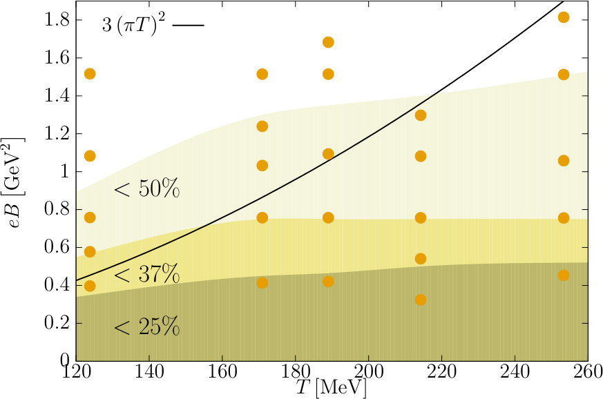 Figure 9
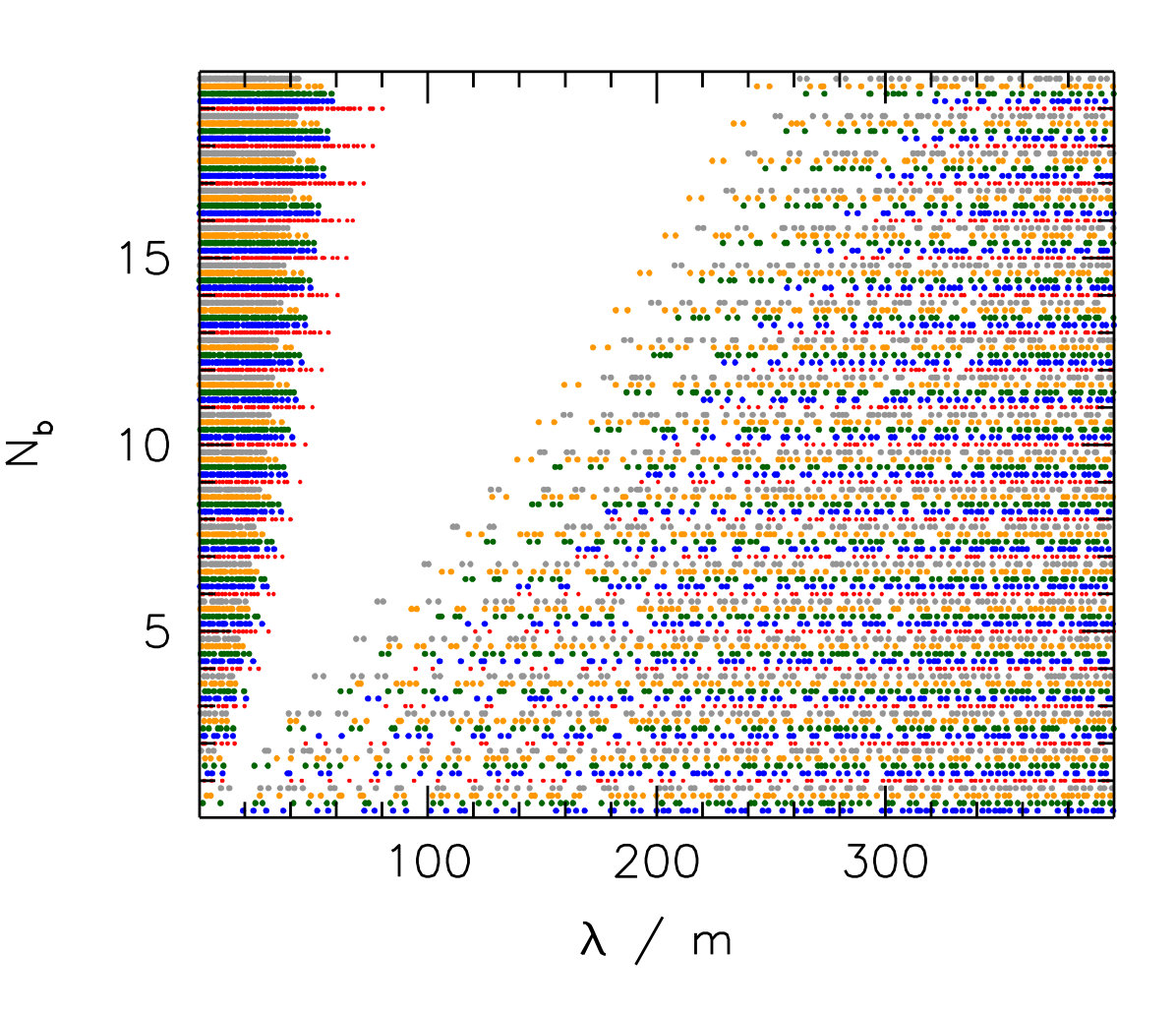 Figure 10
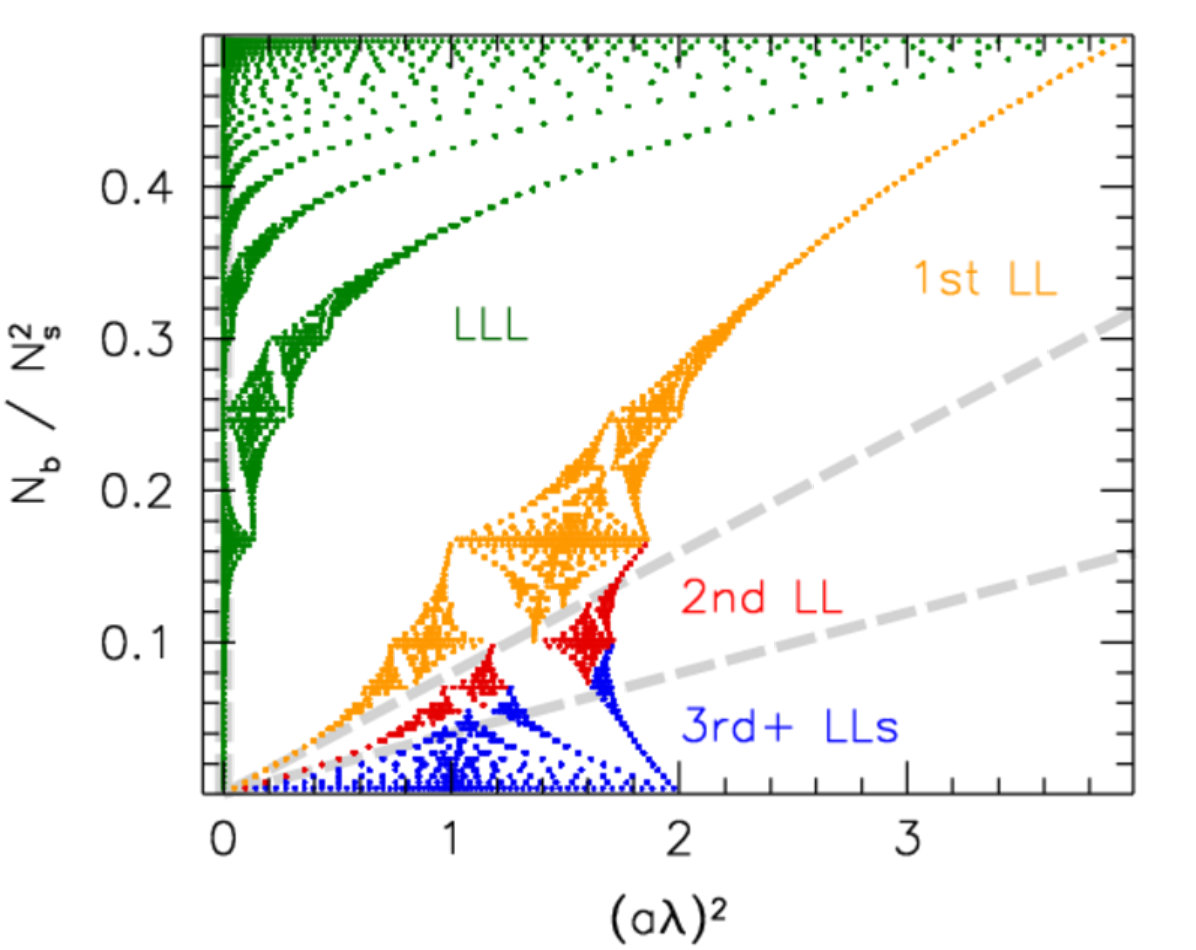 Figure 11
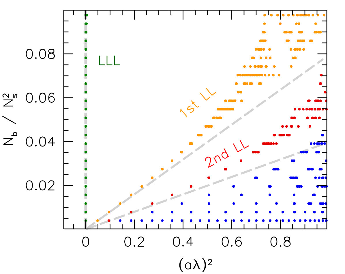 Figure 12
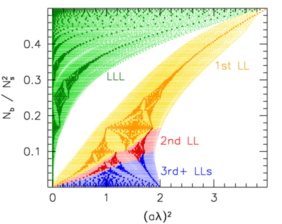 Figure 13
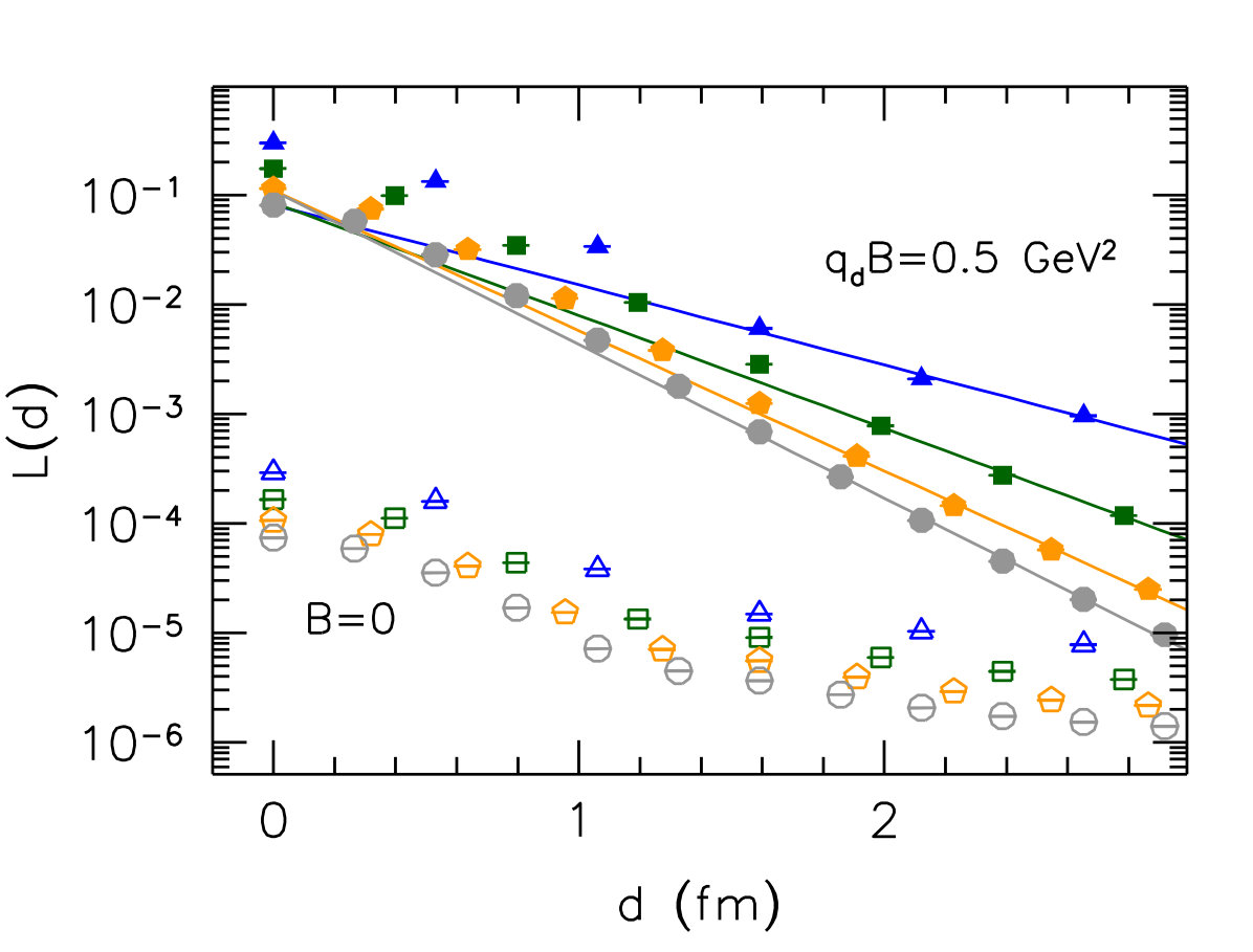 Figure 14
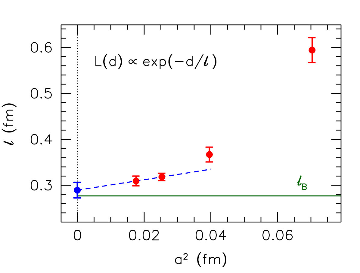 Figure 15
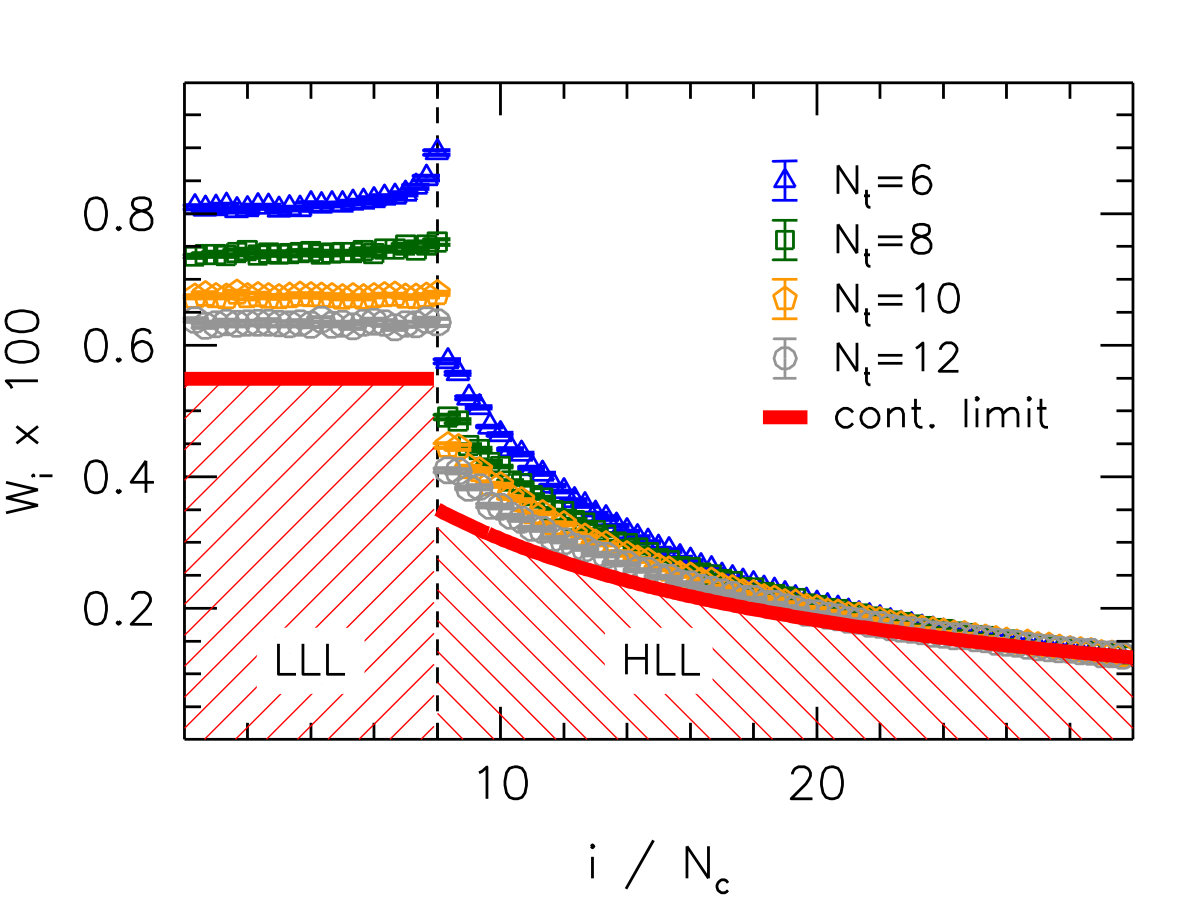 Figure 16
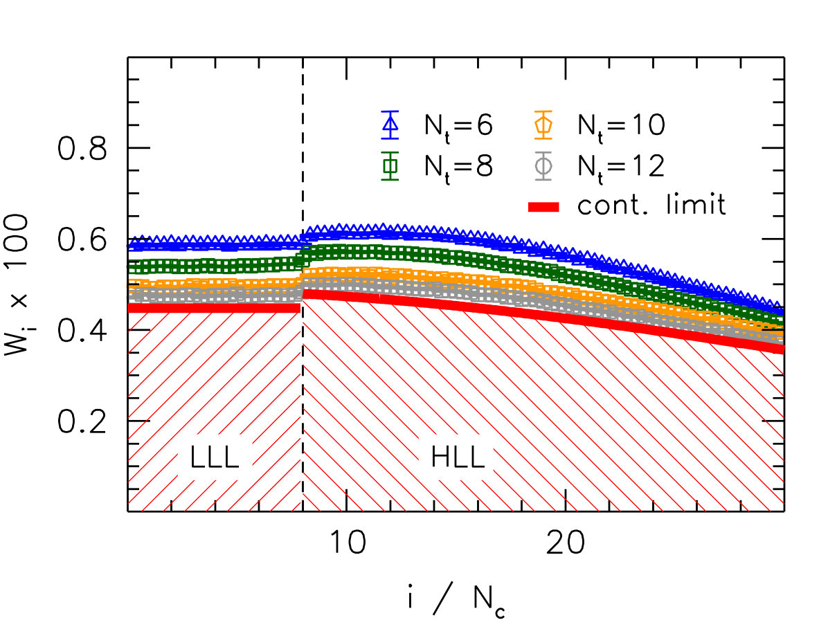 Figure 17
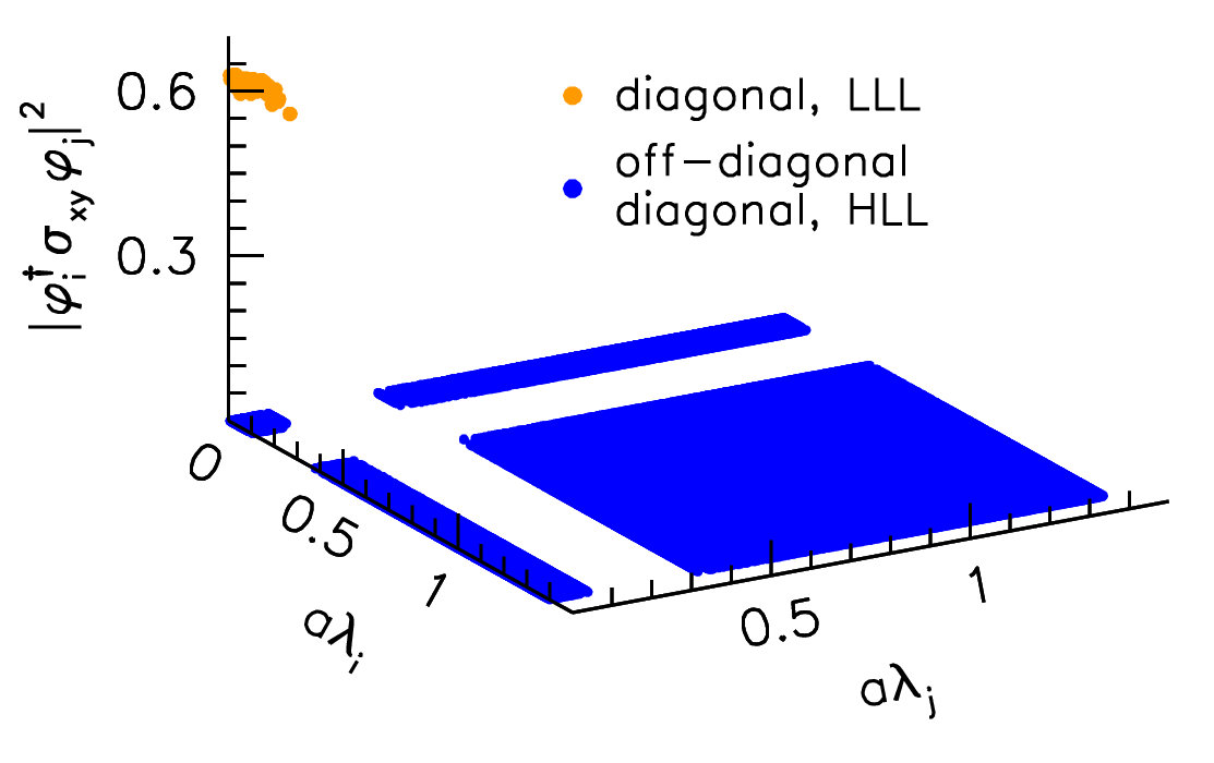 Figure 18
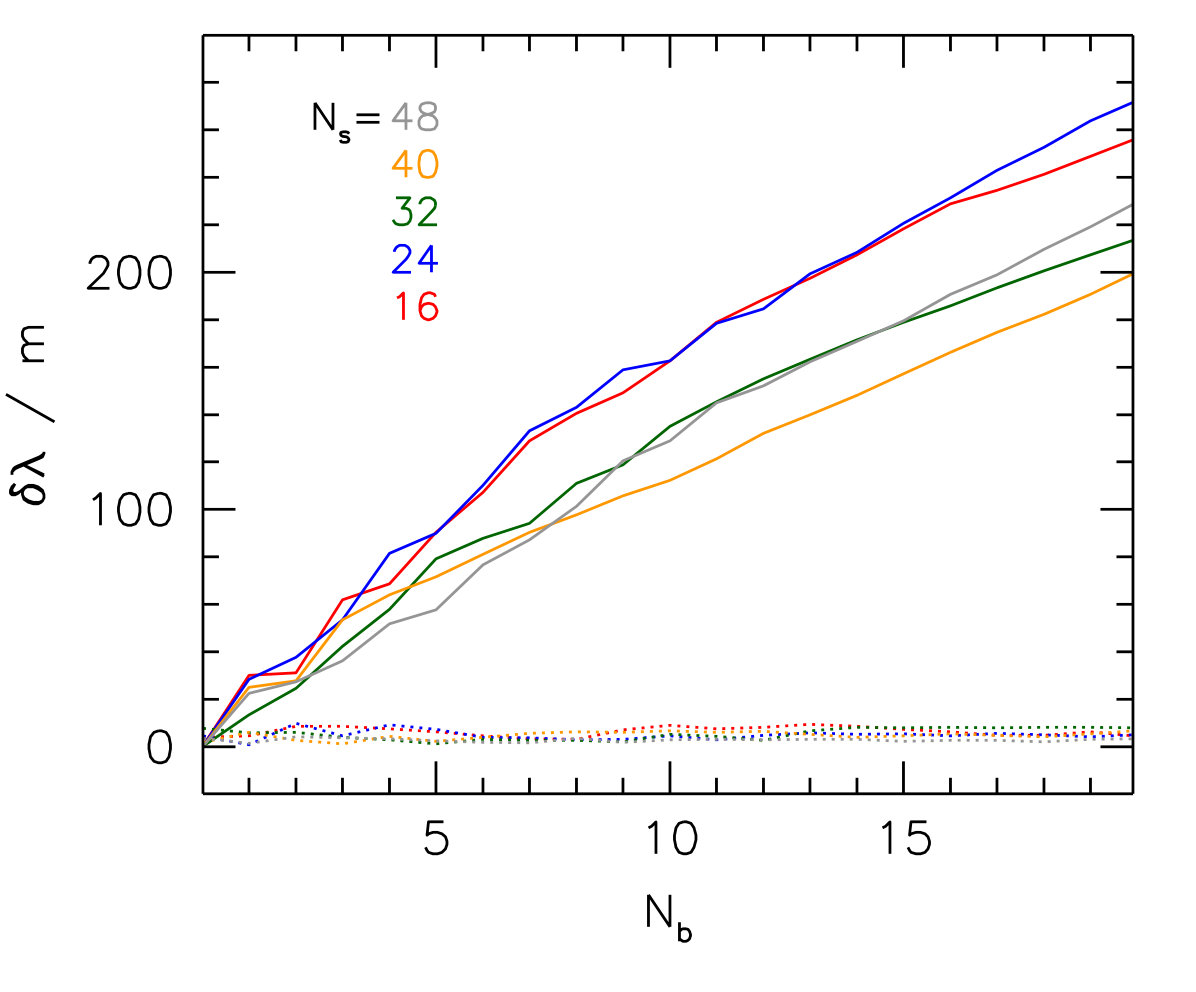 Figure 19
Peer Reviews
No public reviews on file for this paper yet. If you reviewed it on a platform where reviews are public (OpenReview, ICLR, NeurIPS, ICML), you can paste yours below so the community can read it here.
Videos
No videos yet. Explain this paper in a talk, walkthrough, or lecture? Add one.
aainstitutetext: Institute for Theoretical Physics, Universität Regensburg, D-93040 Regensburg, Germany.bbinstitutetext: Institute for Theoretical Physics, Goethe Universität Frankfurt, D-60438 Frankfurt am Main, Germanyccinstitutetext: Eötvös University, Theoretical Physics, Pázmány P. s. 1/A, H-1117, Budapest, Hungary.ddinstitutetext: MTA-ELTE Lendület Lattice Gauge Theory Research Group. Pázmány P. s. 1/A, H-1117, Budapest, Hungary.eeinstitutetext: Institute of Nuclear Research of the Hungarian Academy of Sciences, Bem tér 18/c, H-4026 Debrecen, Hungary.ffinstitutetext: HISKP(Theory), University of Bonn, Nussallee 14-16, D-53115 Bonn, Germany
Landau levels in QCD
F. Bruckmann b
G. Endrődi c,d
M. Giordano c,d
S. D. Katz e
T. G. Kovács f
F. Pittler a
J. Wellnhofer
Abstract
We present first evidence for the Landau level structure of Dirac eigenmodes in full QCD for nonzero background magnetic fields, based on first principles lattice simulations using staggered quarks. Our approach involves the identification of the lowest Landau level modes in two dimensions, where topological arguments ensure a clear separation of these modes from energetically higher states, and an expansion of the full four-dimensional modes in the basis of these two-dimensional states. We evaluate various fermionic observables including the quark condensate and the spin polarization in this basis to find how much the lowest Landau level contributes to them. The results allow for a deeper insight into the dynamics of quarks and gluons in background magnetic fields and may be directly compared to low-energy models of QCD employing the lowest Landau level approximation.
1 Introduction
Background magnetic fields give rise to a wide range of exciting phenomena with applications in solid state physics, cosmology, neutron star physics and heavy-ion phenomenology, see the recent reviews Kharzeev:2013jha ; Miransky:2015ava . Our knowledge about these phenomena is guided by the quantum mechanics of charged particles exposed to background magnetic fields. The motion in this setup is restricted to circular orbits (or spirals) with quantized radii. These so-called Landau levels (LL) are responsible for various effects in solid state physics that involve the electric conductivity or the magnetic moment of the material: the quantum Hall effect, the de Haas-van Alphen effect or the Shubnikov-de Haas effect (see, e.g., Ref. abrikosov1988fundamentals ). The notable features of the Landau spectrum are the separation of the levels proportionally to the magnitude of the magnetic field, and the degeneracy of the levels, proportional to the magnetic flux of the field through the area of the system. In particular, for strong fields the lowest Landau level (LLL) plays the dominant role for macroscopic physics, since higher Landau levels (HLLs) are too energetic to be excited. An additional consequence of the LL-structure is the dimensional reduction of the theory for strong fields, where the motion is restricted to be parallel to the magnetic field.
If is sufficiently large, a weak interaction between the charged particles only perturbs the Landau levels, but leaves the overall hierarchy intact, so that the LLL dominance still holds. In this paper our aim is to investigate whether the concept of Landau levels can also be transferred to strongly interacting quantum field theories and to what extent the LLL dominance persists in this case. In particular, we are interested in Quantum Chromodynamics (QCD), which describes the strong (color) interaction between quarks and gluons. While gluons are electrically neutral, quarks possess electric charge and thus couple directly to the background magnetic field. It is worth emphasizing that the composite particles (e.g. charged pions) of QCD have been observed to exhibit Landau levels Bali:2011qj ; Chang:2015qxa ; Bali:2015vua . While this is expected for these weakly coupled particles, such a hierarchy has never been seen on the level of quarks, which interact strongly among each other. The question of what role quark LLs could play is especially interesting around and above the finite temperature crossover to the quark-gluon plasma, because quark degrees of freedom become more important here.
The most pronounced, magnetic field-induced effect in QCD is the enhancement of dynamical chiral symmetry breaking in the vacuum of the theory Gusynin:1994re ; Gusynin:1995nb . This, so-called magnetic catalysis is one of the most important features of the interaction between quarks, gluons and the magnetic field and has a strong impact on the phase structure of QCD. It is widely believed that the Landau level-structure of the theory – in particular, the dimensional reduction for strong fields – is responsible for magnetic catalysis. This expectation is backed up by calculations in various low-energy approximations, effective theories and perturbative approaches to QCD. For recent reviews, we refer the reader to Refs. Shovkovy:2012zn ; Andersen:2014xxa ; Miransky:2015ava . In addition, a convenient approximation exploiting the separation between the LLL and the HLLs is to neglect all higher levels and only keep contributions from the LLL. This is the LLL approximation, which is widely employed, see, e.g., Refs. Fukushima:2011nu ; Leung:2005xz ; Ferrer:2013noa ; Fayazbakhsh:2010gc ; Blaizot:2012sd ; Ferrer:2014qka ; Fayazbakhsh:2010bh ; Fukushima:2015wck . While the approximation may be justified for strong fields, neglecting the contributions from the HLLs results in systematic effects that are difficult to estimate Kojo:2013uua ; Mueller:2014tea ; Braun:2014fua ; Mueller:2015fka . Notice that certain observables are special in this context as only the LLL contributes to them: this is the case for anomalous currents Fukushima:2008xe and for spin polarizations Frasca:2011zn ; Bali:2012jv (see below).
The Landau level structure has further striking consequences: for vector mesons, the LLL carries a negative contribution to the energy that has been speculated to turn the charged meson massless and, accordingly, the QCD vacuum into a superconductor Chernodub:2010qx . At high baryonic density and low temperature the gradual enhancement of the Fermi energy results in a consecutive filling of the individual Landau levels and related oscillations. The characteristic filling of the LLL was found to remain stable against color interactions using holography Preis:2010cq .
Yet another motivation to understand the role of Landau levels comes from the structure of the QCD phase diagram for nonzero magnetic fields. Lattice simulations have revealed Bali:2011qj ; Bali:2012zg ; Endrodi:2015oba (see also Ref. Bornyakov:2013eya ) that around the deconfinement/chiral symmetry restoration transition of QCD, the quark condensate is reduced by the magnetic field (inverse magnetic catalysis) – an unexpected result if we compare it to the discussion above about the robust nature of magnetic catalysis. The impact of the LLL for inverse magnetic catalysis has been addressed, e.g., in Ref. Ferrer:2014qka . For a review on approaches to describe this phenomenon, see Refs. Fraga:2012rr ; Andersen:2014xxa .
In this paper we identify, for the first time, the Landau level-structure of the quark Dirac operator on the lattice. After defining the Landau levels in detail in Sec. 2, we describe our method to separate the lowest Landau level and the higher Landau levels in two and in four dimensions. In Sec. 3 we define the LLL-contribution to certain QCD observables including the quark condensate and the spin polarization. This is followed by Sec. 4, where we quantify the difference between the LLL and the full theory for various magnetic fields and temperatures. The observables and their divergences are calculated analytically in the free case in the appendices. Finally, Sec. 5 contains our conclusions. Our preliminary results have been published in Ref. Bruckmann:2016bcl .
2 Landau levels
First of all we need to define Landau levels more specifically. It is instructive to begin the discussion in two spatial dimensions and then proceed to the physical case of space-time dimensions. In addition, for each dimensionality we first describe the levels in the free theory, where quarks only interact with the magnetic field but not with gluons. Then, by switching on the strong interactions we can analyze whether the levels remain intact or if they are mixed.
2.1 Two dimensions
Let us consider a quark with electric charge that interacts with a background magnetic field but is otherwise free. In the following we will refer to this simply as the “free case”. We work with natural units and assume for simplicity , and that the magnetic field points in the direction. In a finite periodic box of area in the plane, the flux of the magnetic field is quantized 'tHooft:1979uj ; AlHashimi:2008hr so that for the flux quantum the following condition is satisfied:
[TABLE]
The two-dimensional Dirac equation for such a background involves a coupling of both to the spin and to the angular momentum of the quark. These operators have quantized eigenvalues and with . The eigenvalues of the massless Dirac operator (times ) will be referred to as energy levels. The squared energies and their degeneracy read
[TABLE]
where we combined the angular momentum and spin into a single quantum number and denotes the number of colors. These levels are called Landau levels and is the Landau index. Notice that since the contribution of the lowest angular momentum is exactly canceled by , the energy of the lowest Landau level (LLL) with is zero independently of . In addition, the LLL is the only level that has well-defined spin – for our positively charged quark the spin is aligned with the magnetic field, (and the angular momentum vanishes). In contrast, higher Landau levels (HLLs) have no definite spin. In the following we will index the eigenmodes either by the pair with labelling the Landau levels and labelling the degenerate modes within each level, or simply by an integer running over all the modes (ordered according to the eigenvalues).
Next, we discretize space on a symmetric lattice with points and a lattice spacing using the staggered Dirac operator. This formulation entails a twofold doubling of the squared eigenvalues. In addition, the lattice puts an upper limit on the allowed maximal magnetic field and the quantization condition (1) becomes
[TABLE]
The spectrum in this setting is shown in the left panel of Fig. 1. The discretized system is near the continuum limit if the lattice is sufficiently fine to resolve the magnetic field: , i.e. . The right panel of Fig. 1 shows that this is indeed the case: for low flux quanta the eigenvalues of the lattice Dirac operator are on top of the continuum curves (2). For higher values of , the Landau level hierarchy is broken by discretization artefacts so that the spectrum spreads around the continuum energies. This spread proceeds in an apparently recursive manner, with the large-scale structure of the spectrum being repeated on ever smaller scales. The so emerging fractal is a well-known object in solid state physics and is called Hofstadter’s butterfly Hofstadter:1976zz .
The butterfly has many spectacular features, some of which also persist (at least partially) if QCD interactions are switched on Endrodi:2014vza . Here we concentrate on one of these characteristics: the structure of the gaps in the spectrum. The color coding of the eigenvalues in the left panel of Fig. 1 corresponds to the continuum degeneracy (2) – ordering the eigenvalues according to their magnitude, the first entries are assigned to the lowest (zeroth) LL, the next entries to the first LL and so on. The factor of two is included to take into account the twofold fermion doubling mentioned above. Interestingly, this classification exactly coincides with the separation in terms of the gaps. Another feature of the lattice spectrum is that the eigenvalues are always below their corresponding continuum Landau levels – with the exception of the zeroth level, see the left panel of Fig. 1.
Next we switch on QCD interactions by taking one slice of a four-dimensional QCD gauge configuration and inserting the links in the two-dimensional staggered Dirac operator . Thereby two new scales are introduced in the system: the strong scale and the temperature . In particular, here we consider a lattice from an ensemble generated at . Notice that the minimal magnetic fields (i.e. small ) are then comparable to and to so that a nontrivial competition between these scales is expected to take place. The so obtained spectrum is shown in the left panel of Fig. 2, revealing that – as expected – the butterfly is smeared out by the color interactions. Nevertheless, two crucial aspects of the lattice spectrum remain unaltered: a) the distinct presence of the largest gap and b) the correspondence of the left and right hand sides of the gap to LLL and to HLLs, respectively, based on the continuum degeneracies. These two features enable us to unambiguously separate the LLL from HLLs in two-dimensional QCD.
Notice also that the smaller gaps between HLLs are closed by the interactions, such that a similar distinction between, say, the first and the second Landau level is not obvious. The LLL remains separate due to topological reasons. Namely, the topological charge in two dimensions is just the magnetic flux (even in the presence of non-Abelian interactions)
[TABLE]
and the usual four-dimensional notion of handedness is replaced by the spin direction, thus the index theorem entails that equals the difference of the number of spin-up and spin-down polarized zero modes. In addition, in two dimensions the ‘vanishing theorem’ Kiskis:1977vh ; Nielsen:1977aw ; Ansourian:1977qe ensures that either or is zero. Thus, for the only states in the spectrum with definite spin have spin up and according to Eq. (4) . Indeed, the LLL eigenvalues vanish in the continuum111In the staggered discretization the LLL modes are not real zero modes but are well separated from the HLL eigenvalues. In the overlap formulation Neuberger:1997fp ; Neuberger:1998wv these modes become exact zero modes., and their degeneracy is (for each color).
To demonstrate that even in the presence of color interactions the LLL only accommodates spin-up states, in the right panel of Fig. 2 we plot the squared matrix elements of the spin operator222The staggered discretization of the spin operator is detailed in Ref. Bali:2012jv . for the down quark at a magnetic flux quantum . Besides the separation of the LLL modes () from the HLL modes (), the two sets are also clearly distinguished by their spin matrix element. In particular, we find that is almost perfectly diagonal in the eigenmode basis – the off-diagonal matrix elements are below . For the diagonal elements, the HLL entries are also suppressed (below ), while the LLL entries are much larger, in this case around . In fact, the spin of the LLL modes approaches unity in the continuum limit. Thus, the classification of the two-dimensional modes based on their mode number (LLL degeneracy) coincides with the classification based on their spin.
It is therefore the index theorem that protects the LLL states from mixing with HLL modes, resulting in the persistence of the gap even in the presence of QCD interactions. To show that the above characteristics remain to hold in the continuum limit, we plot the gap for various lattice spacings in a fixed physical volume in the left panel of Fig. 3. The employed QCD configurations are two-dimensional slices of typical high-temperature () four-dimensional gauge configurations with aspect ratio and . The gap is shown this time in physical units: the magnetic flux on the horizontal and the eigenvalue in units of the bare quark mass on the vertical axis.333This choice of normalization is dictated by the fact that expressing the eigenvalues in units of the bare quark mass leads to a renormalization-group-invariant spectral density Giusti:2008vb , and is thus required to obtain a meaningful continuum limit. Apparently, the gap edges remain well-defined also in the limit (i.e. ). To be more specific, in the right panel of the same figure we plot the width of the gap as a function of , together with the eigenvalue spacing just above the gap. We see that the gap width always largely exceeds the typical spacing – in other words, the gap at small flux quanta is indeed a well-defined physical structure that survives the continuum limit. Notice moreover that as the continuum limit is approached, the LLL states – while having a fixed multiplicity – are compressed towards zero, in accordance with their would-be-zero-mode nature. Finally we remark that above we presented the pronounced features of the spectrum using high-temperature QCD ensembles, but our main conclusions remain unchanged if we use instead gauge configurations in the confined phase.
2.2 Four dimensions
Next, we generalize the concept of Landau levels to four dimensions in Euclidean spacetime. In the absence of color interactions, the Dirac equation for the and coordinates decouples from the Landau problem in the plane and has free wave solutions with momenta and . Thus, the eigenmodes factorize as , where labels the LL and the degenerate modes within each level. The squared eigenvalues and their degeneracies read
[TABLE]
(Here we assumed strictly zero temperature, i.e. an infinite size in the temporal direction.) Therefore, each Landau level has become an infinite tower of states, involving all the allowed momenta in the and directions. As a consequence, it is not possible anymore to separate the LLL from the HLLs just by looking at the eigenvalues . Clearly, we need to extract the Landau index from the eigenmode, or, in other words, work with a projector that projects onto the subspace spanned by the modes with the lowest Landau index ,
[TABLE]
On the lattice, the eigenmodes still factorize as (here runs over all the two-dimensional modes, see our remark after Eq. (2)). Instead of using the plane wave basis in the and directions, we can also span the same space by using the coordinate basis consisting of states localized at a single value of and of ,
[TABLE]
After ordering the according to their eigenvalues, the first two-dimensional states correspond to the LLL (see Fig. 1). Therefore, a valid way to rewrite (6) is to only include these modes,
[TABLE]
where the sum over doublers appears due to the twofold doubling of staggered fermions in two dimensions.
If QCD interactions are switched on, the components of the four-dimensional Dirac operator in general do not commute, i.e. the eigenmodes do not factorize as in the free case above. Nevertheless, we may still employ the basis of the eigenstates of for each plane of the lattice, labelled by the coordinates . The factorized modes are built up from these, similarly as in Eq. (7),
[TABLE]
Thus, the projection in this setting reads
[TABLE]
This is the projector we will use in full four-dimensional QCD to pick out the states corresponding to the LLL. Later we will also use the same construction but composed of the eigenmodes of the two-dimensional Dirac operator at vanishing magnetic field. Similarly as above, this uses and reads
[TABLE]
Once again, involves the same number of modes as does, but the modes are eigenstates of the Dirac operator.
Our numerical results will show that the four-dimensional modes of never correspond purely to the LLL or to a HLL but instead – owing to the mixing between the various planes via gluon fields in the and directions – have overlap both with and with its complement . Nevertheless, for typical low-lying four-dimensional modes, there is a distinct jump in the overlap with between and i.e. just at the border of the LLL.
This is visualized in the left panel of Fig. 4 for normalized four-dimensional modes for the down quark () at . We define the overlap factor as
[TABLE]
where the sum also includes the two two-dimensional doublers and the scalar product involves a sum over all lattice points. The completeness of the modes ensures that the normalization is . We average over four-dimensional modes in a small spectral interval and over several gauge configurations. The magnetic flux used here is , leading to a LLL degeneracy of . The left panel of Fig. 4 reveals that low-lying modes tend to have larger overlap with two-dimensional LLL modes than with HLL states. also remains constant in the LLL region , suggesting the equivalence of all two-dimensional lowest Landau levels in this respect. This feature, together with the drastic downward jump at the end of the LLL region remains pronounced even in the continuum limit.
In the right panel of Fig. 4 we plot the same quantity, only this time are high-lying four dimensional modes that are expected to have less overlap with the LLL. Indeed, the pronounced downward jump becomes a slight upward jump, so that these modes can be rather thought of as being HLL-dominated. We also mention that the structures visible in Fig. 4 disappear for and the overlap becomes a smooth, monotonically decreasing function.
Another important aspect regarding LLL-projected fermions is the locality of the fermion action corresponding to the Dirac operator restricted to the LLL subspace. Note that already in the continuum, the lowest Landau level spreads over a range in the plane perpendicular to the magnetic field (see, e.g., Ref. Miransky:2015ava ), so that the LLL-projected quark action involves (contrary to usual QCD) the product of quark fields smeared over the range . A nontrivial check of our lattice construction is whether this localization range is reproduced. The original Dirac operator without the projection is ultralocal as it only uses nearest neighbor links. Thus, for LLL-projected fermions we need to check the locality of the projector itself. As can be seen directly from Eqs. (9) and (10), is ultralocal in the and directions. To discuss locality in the plane, we consider a source vector localized at the point and the vector obtained by projecting with . We measure , with the distance from the source in the plane. As the left panel of Fig. 5 reveals, this quantity falls off exponentially with the distance, signaling that interactions between sufficiently separated quark fields are indeed suppressed – once the averaging over gluonic configurations is performed. In the right panel of Fig. 5 we perform the extrapolation of the decay length and find that in the continuum limit it is indeed consistent with the expected value for the magnetic field considered here. We emphasize that the locality of (in the sense described above) is a highly nontrivial finding that arises from the interplay of the LLL modes.444We mention that the locality of the action in lattice units (i.e., for ) for usual QCD is a prerequisite for the universality of the continuum limit. For the LLL-projected action the microscopic details of the discretization are damped by the magnetic localization length, present even in the continuum theory. Strictly speaking, the universality argument can therefore only be applied for where . In general, the projection onto a subset of eigenmodes of the Dirac operator is a highly nonlocal object. We demonstrate this by applying the same construction at – building the projector of Eq. (11) from the lowest two-dimensional modes at vanishing magnetic field. The so obtained object does not appear to exhibit exponential decay, see the left panel of Fig. 5.
3 Observables
Having prescribed the procedure to project an arbitrary four-dimensional mode to the LLL sector, we are in the position to test to what extent certain QCD observables are LLL dominated. We work with three quark flavors indexed by . The observables can be derived from the QCD partition function , which is written using the Euclidean path integral over gluon and quark fields ,
[TABLE]
where and are the gluonic and fermionic actions, respectively, and with flavor blocks denotes the quark matrix. The Dirac operator is flavor-dependent due to the different electric charges: with the elementary charge. Integrating out the fermion fields analytically, the expectation values of quark bilinears for the flavor read
[TABLE]
Here, the rooting trick for staggered quarks is employed to reduce the number of flavors to three in the continuum limit and the division by the four-volume renders the observable intensive. The details of our lattice setup, including the simulation algorithm, the implementation of the magnetic field and the line of constant physics to set the quark masses and are described in Refs. Borsanyi:2010cj ; Bali:2011qj .
To find the LLL contribution to the observable (14), we work with the projector of Eq. (10), which projects onto the subspace spanned by all of the two-dimensional LLL modes (defined on two-dimensional slices corresponding to all values of and of ). The projector is a block-diagonal matrix in flavor space, . The LLL projection amounts essentially to replacing the fermion matrix by its projected version . After integrating out the fermions, shows up both in the trace and in the determinant in Eq. (14). One can then consider the effect of the LLL projection on the valence quarks in the operator in question – represented by the trace – as well as on the sea quarks that characterize the distribution of the gluonic configurations – represented by the determinant. In the present approach, we only insert the projector in the valence sector. The sea contribution is considerably more complicated to implement and we leave it to a forthcoming study.555Here we mention only that if one wants to insert in the determinant, one should also “quench” the HLL modes, i.e., the correct replacement would be . Similarly, we only insert the magnetic field in the valence Dirac operator and exclude in the sea sector, i.e., for the generation of the gauge configurations. This implies that valence quarks feel the magnetic field and are projected to the LLL, while virtual sea quarks behave as if they were electrically neutral. We mention that the valence contribution is dominant for, e.g., the quark condensate at low temperatures DElia:2011koc but not around the QCD transition Bruckmann:2013oba . This should be kept in mind in the following.
Our definition of the full and the LLL projected quark bilinears (in the valence approximation) thus reads
[TABLE]
The traces are evaluated using noisy estimators . For the LLL projected observable, this amounts to
[TABLE]
where is taken from Eq. (10) for the flavor and we used and the cyclicity of the trace. In the following we consider the quark condensate and the spin polarization and refer to these by the superscripts and (for scalar and tensor, respectively). The staggered discretization of the spin operator involves gauge links lying in the plane and is detailed in Ref. Bali:2012jv .
Besides the representation of the traces using noisy estimators (which we use below to determine the observables), it is instructive to discuss their relation to the overlap of the four dimensional modes with the basis modes carrying the two dimensional index , defined in Eq. (12) and visualized in Fig. 4. To see this relation, we use the eigenmode basis of the four-dimensional Dirac operator . In this representation, the LLL-projected bilinears read
[TABLE]
where we used the symmetry of that its eigenvalues appear in complex conjugate pairs. The spin operator is diagonal in the and coordinates, which allowed us to rewrite the matrix element in the second relation using the two-dimensional modes and the block living on the slice . In the first step of the second relation we used the fact that is to a good approximation diagonal in the two dimensional modes even in the presence of color interactions, see the right panel of Fig. 2. Moreover, in the second step we approximated the matrix element of on the two-dimensional modes to be independent of the coordinates , which we find to hold if the average over gluon configurations is performed.
In contrast to the LLL-projected observables of Eq. (17), the full observables involve a sum over all values of . The left panel of Fig. 4 tells us that the contribution of the overlaps to the total is enhanced for low-lying modes . Naively, this works in favor of the LLL dominance of the condensate, however, also contains ultraviolet divergent contributions so that a sensible comparison of the LLL-projected and the full observables necessitates renormalization. The situation is similar for the spin polarization. In addition to the overlaps , here the matrix elements for are also much larger than for higher , see the right panel of Fig. 2, which (again, naively) enhances the LLL-dominance for this observable even further. Our next step is therefore the renormalization of both observables, which we discuss in the next subsection.
3.1 Renormalization
Both and contain additive as well as multiplicative divergences. However, it turns out that somewhat different renormalization procedures are required for the condensate and for the spin polarization.
Let us consider first. As the analytic calculation in the free case reveals (see App. A), the LLL projected and the full condensates contain different divergences (logarithmic for the former and logarithmic plus quadratic divergences in the cutoff for the latter). Thus, simply taking the difference of the two quantities is not sufficient to cancel these terms. Instead, we consider two different routes to deal with these divergences.
First, we use the gradient flow of the gauge fields to make both the LLL projected and the full observables ultraviolet finite. This procedure smears the gluon Luscher:2010iy and the fermion Luscher:2013cpa fields over a smearing range and thereby eliminates ultraviolet noise and with that the additive divergent contribution to physical quantities. The smearing radius is in spirit similar to a momentum cutoff . We choose the magnetic field to set the smearing range: with and check that the results depend only mildly on . Our implementation of the gluonic and fermionic flow for staggered quarks is detailed in Ref. Bali:2014vja . The so renormalized observable reads
[TABLE]
The second approach does not involve additional ultraviolet cutoffs like the smearing radius above. Instead, the additive divergences are canceled here by taking the difference between the expectation values at and at . For the full condensate this is a straightforward procedure that gives the change of the condensate due to the magnetic field,
[TABLE]
For the LLL projected condensate it is somewhat less obvious how to define this difference. The analysis of the free case (see App. B) reveals that the divergences can be canceled if one performs a similar projection in the term as well, which involves the projector of Eq. (11), built from the eigenmodes of the Dirac operator. We then define the subtracted LLL condensate as
[TABLE]
We emphasize that in the term the projector projects on the lowest eigenmodes of the two-dimensional Dirac operator. In the term, projects on the same number of modes, but this time of the Dirac operator. Using this construction, our second ratio reads666Notice that involves the projector , which – according to the discussion at the end of Sec. 2.2 – corresponds to a nonlocal operator and might complicate the continuum limit of . From this point of view, the first ratio is more advantageous. Nevertheless, below in Sec. 4 we will find that both and give similar results.
[TABLE]
For the spin polarization (superscript ), the ratio can be defined using the same prescription as for the condensate,
[TABLE]
The ratio must be defined differently, since vanishes identically at . Namely, in the absence of the magnetic field, there is no preferred direction and the spin polarization averages to zero. However, we can exploit the fact that the divergences of the LLL and of the full observable coincide this time. This is supported by the calculation in the free case in App. A. This divergent piece, denoted by , has been determined777In fact, the determination of in Ref. Bali:2012jv was carried out with the magnetic field both in the valence and in the sea sector taken into account. This we checked to be a sub-percent effect compared to at low temperatures, but becomes increasingly important as grows and the expectation value reduces. We find that the systematic error in due to neglecting the sea contribution is much smaller than lattice artefacts for our lowest two temperatures and so in the following we only consider these simulation points for . at zero temperature in Ref. Bali:2012jv using the method summarized in App. A. Therefore we have
[TABLE]
Let us now turn to the multiplicative renormalization. The renormalization constants are expexted to be independent of the magnetic field, and the LLL-approximation is assumed to accurately describe strong magnetic fields. Thus it seems natural to assume that the renormalization constants in the full theory and for the LLL coincide, and ratios of the LLL-projected and the full observables – like and above – are free of multiplicative divergences. However, since defining the LLL-projection on a finite lattice effectively involves the asymptotic limit before the continuum limit – i.e. with the magnetic field exceeding even the cutoff – the ultraviolet behavior might still be affected. Whether this is the case should be checked in the future. For this reason, in the present paper we do not perform a continuum extrapolation of our results but merely show data obtained using different cutoffs.
4 Results
We have performed measurements for a range of temperatures and magnetic fields using four lattice ensembles with and . These serve to approach the continuum limit at a fixed temperature owing to . Thus, the larger , the closer we are to the continuum. The aspect ratios were set to to keep the physical volume fixed. Throughout the rest of this section we consider the down quark flavor . Since we only implement the magnetic field and the LLL-projector in the valence sector, for the bilinears for the up quark we identically have (here we also exploited parity symmetry ).
We begin the presentation of the results with the quark condensate. The two ratios and of Eqs. (18) and (21) are plotted in Fig. 6 for two temperatures, below and above the finite temperature QCD crossover. Both combinations give similar results, rising from about to within the range . The ratios are expected to approach unity for strong magnetic fields, as the analytic calculation in the free case shows (see App. B). In the figures we also include the vertical line to indicate the point where the magnetic field (times the modulus of the electric charge ) becomes the largest dimensionful scale in the theory. We measured with smearing radii and and found that the systematic effect due to varying in this range is much smaller than the lattice artefacts.
While for the ratio renormalized through the gradient flow, our and results still significantly differ, shows nice scaling towards the continuum limit. As grows and the magnetic field in lattice units increases, lattice artefacts are expected to become more pronounced, as visible in the right panels of Fig. 6. In the following we will take the results for as a reference for the validity of the LLL-approximation. The LLL-contribution to this observable reaches 60% at our largest magnetic field and seems to further increase towards unity rather slowly. This is in agreement with the free case, where the deviation from 1 is of the form for large , see Eq. (42).
Next we turn to the spin polarization. The renormalized ratios and were defined in Eqs. (22) and (23) above. We plot both in Fig. 7 as functions of the magnetic field for the two temperatures that we considered above. Just as for the condensate, the ratio exhibits faster scaling towards the continuum limit. We find that i.e., the spin polarization is overestimated by the LLL approximation (for this trend is not obvious due to large cutoff effects). This may be understood by noting that is a traceless operator and that has matrix elements close to unity on the LLL-modes (see Fig. 2). Thus, the higher modes must have negative matrix elements so that the total trace can vanish and, accordingly, the HLL contribution to is negative. The deviation of from unity is much milder than for the condensate, remaining below for our finest lattices for the complete range of magnetic fields that we consider here. Notice that the LLL-approximation is expected to work well for this observable since in the free case the HLL-contribution to vanishes identically (see App. B).
5 Summary
In this paper we investigated the validity of the lowest-Landau-level (LLL) approximation to QCD in the presence of background magnetic fields. In the absence of color interactions, this approximation is based on the structure of the analytically calculable energy levels (the Landau levels) of the quantum system. While the energy of the lowest level is independent of , the higher levels have squared energies above and thus become negligible if the magnetic field is sufficiently strong. Furthermore, the characteristic degeneracy of the Landau levels is proportional to the magnetic flux.
The presence of (nonperturbative) color interactions mixes the levels and therefore complicates this simple picture considerably. In the present paper we demonstrated, for the first time, that the lowest Landau level can nevertheless be defined in a consistent manner even for strongly interacting quarks. The definition of the LLL is based on a two-dimensional topological argument that characterizes the plane (the plane perpendicular to the magnetic field). Namely, the two-dimensional LLL modes have zero energy and their number is a topological invariant fixed by the flux of the magnetic field, independently of the gluonic field configuration. Although these exact zero modes are shifted to nonzero values on a finite lattice, they are still well separated from the rest by a gap in the spectrum. We have shown that this gap is a remnant of the largest gap in the fractal structure usually referred to as Hofstadter’s butterfly in the Hofstadter (lattice) model of solid state physics.
This construction can be performed on each plane, i.e., for each value of the and spacetime-coordinates. While the two-dimensional modes can be unambiguously classified as belonging or not to the LLL, in four dimensions this is not the case anymore: a general four-dimensional Dirac eigenmode has overlap both in and out of the LLL. We defined the projector that projects the four-dimensional modes onto the subspace of two-dimensional LLL modes for each and . Using the projector, we have shown that low-lying four dimensional modes have enhanced overlap with the LLL. For higher four-dimensional modes the overlap with LLL is instead suppressed with respect to HLLs.
Motivated by this, the LLL contribution to standard fermionic observables can be determined. In particular, we concentrated on the quark condensate and the spin polarization for the down quark. We constructed ratios of the LLL-projected and the full observables that are free of additive divergences (demonstrated in the free case in App. A) and that approach unity in the limit (shown in the free case in App. B).
Our results indicate that the LLL approximation underestimates the quark condensate and overestimates the spin polarization. In addition, the LLL-projected quantities slowly approach the full observables as the magnetic field grows and exceeds further dimensionful scales and in the system. Our final results for the condensate (using the data for ) are visualized for a wide range of temperatures in Fig. 8. In this figure the validity of the LLL-approximation is represented in the plane. Dark colors stand for regions where the approximation breaks down in the sense that the LLL-projected condensate is far away from its full value (so that is less then , or ). The white region is where the LLL-contribution to the condensate amounts to more than half of the full condensate. The contours were determined by means of a spline interpolation of to calculate the magnetic fields where the observable reaches a given percent. Using these threshold magnetic fields for each temperature, a second set of spline interpolations results in continuous -dependent functions that are shown in the contour plot. The so obtained contours may be compared to the naive expectation , also indicated in the figure.
Summarizing, we have quantified the systematics of the LLL approximation via first-principle lattice simulations of QCD with background magnetic fields. The results may be compared directly to low-energy models or effective theories employing only the lowest Landau level. We emphasize that our findings correspond to the valence sector, i.e. only the quark fields in the operators and are projected to the LLL but not the virtual sea quarks appearing in loops. The extension of the approach to sea quarks is more involved and is left for a future study.
Acknowledgements.
This research was supported by the DFG (Emmy Noether Programme EN 1064/2- 1, SFB/TRR 55, BR 2872/6-1, BR 2872/6-2 and BR 2872/7-1), by OTKA (OTKA-K-113034) and by the Hungarian Academy of Sciences under “Lendület” (No. LP2011-011). GE is grateful for the hospitality of the organizers of the Workshop on Magnetic Fields in Hadron Physics 2016, where early results of our work were presented and discussed.
Appendix A Additive divergences in the free case
In this appendix we calculate the additive divergences of the fermion bilinears in the free case and demonstrate that the ratios and of Eqs. (18), (21), (22) and (23) are ultraviolet finite. We work in a finite but large volume , orient the magnetic field in the positive direction and assume that . Since the divergences are independent of the temperature, we will work at . Throughout the appendices we will neglect a factor , since in the free case all colors give the same contribution.
The quark condensate in the free case (four dimensions, no LLL projection yet) can easily be shown to have the following spectral representation (see e.g. App. B in Bali:2012jv ):
[TABLE]
where in the third equality we used the existence of chiral partners with opposite eigenvalue . The eigenvalues and the degeneracies are given in Eq. (5). For the sum over Matsubara frequencies turns into an analogous integral over . The combined momentum integration/summation over and is UV divergent for fixed . Therefore, the condensate is divergent for the LLL projected as well as for the full case.
We can make this divergence more transparent with the help of Schwinger’s proper time Schwinger:1951nm . In our case this simply amounts to using the identity to exponentiate making it possible to sum over the Landau levels and to integrate over the momenta,
[TABLE]
The quantity has dimension and thus the UV divergence occurs at the lower end of the integral, where
[TABLE]
Since both of the divergent terms are -independent, the additive divergence in the condensate can be removed by subtracting the condensate.
The LLL projected condensate follows easily by setting above instead of summing over , or, equivalently, by replacing by 1. We obtain
[TABLE]
Consequently, the divergence is weaker:
[TABLE]
The magnetic field occurs only as an overall factor, and the LLL projected condensate would vanish for , where indeed the notion of Landau levels is meaningless. The additive divergence can be canceled by subtracting the fermion bilinear involving the projector defined at , see App. B below.
Another way of regularizing the observables is the gradient flow method Luscher:2010iy ; Luscher:2013cpa . There the fields are flowed/smeared with the help of the heat kernel
[TABLE]
where is the gauge-covariant Laplace operator and is the flow time, of dimension . Note that is nonnegative. In the condensate, two quark fields are flowed, thus
[TABLE]
Note that the argument is related to the smearing radius introduced in Eq. (18) in the main text as Luscher:2010iy .
For the evaluation of the free flowed condensate we note that the free Laplacian commutes with and its eigenvalues are those of the latter, Eq. (2) and (5), with the spin set to zero, i.e., with quantum number and the corresponding degeneracy
[TABLE]
The contributions of the chiral partners to the condensate can be taken into account as before, and thus we obtain the spectral representation
[TABLE]
Also here we can make use of Schwinger’s proper time, which yields
[TABLE]
Clearly, the flow time regularizes the integral for small values of the proper time , and is hence equivalent to a UV-cutoff in momentum space or a smearing radius in coordinate space. In the LLL approximation the flowed condensate is obtained by taking only the contribution to the full condensate:
[TABLE]
For the LLL approximation to make sense, should be the largest scale in the system. Therefore we choose for the flow time or, equivalently, for the smearing radius , with . Note that this choice has a well defined continuum limit for fixed , as the physical smearing radius is kept fixed by .
The other observable we consider is the spin polarization . Following Eq. (24) we obtain
[TABLE]
where in the last two equalities we have used that the expectation value, , is only non-vanishing in the lowest Landau level. Thus in the free case the spin polarization is made up purely by the LLL-contribution. Both are equal to Eq. (28) and are thus logarithmically divergent. Since the divergence is proportional to , a possible way to separate the infinite part is via Bali:2012jv
[TABLE]
This prescription can also be applied in the interacting case and has been measured in full QCD in Ref. Bali:2012jv .
Appendix B -dependence of the ratios in the free case
In this appendix we discuss the magnetic field-dependence of the ratios and in the free case. We again assume that and neglect an overall factor of . First we consider the ratio of Eq. (21) for the quark condensate,
[TABLE]
where the projector , defined in Eq. (11), involves the lowest two-dimensional modes (for each slice), with given by the flux quantum that corresponds to the finite term. We discuss here the case in detail.
In the free case the denominator reads, cf. Eqs. (25) and (27) with variable change ,
[TABLE]
where . The numerator is the difference
[TABLE]
which turns out to be UV finite. Here we subtract the contribution of the lowest modes from the LLL contribution. To see why is the correct value for the upper limit, consider the number of two-dimensional fermionic quantum states at in a finite box ,
[TABLE]
Performing the integrals we obtain
[TABLE]
and with Eq. (38):
[TABLE]
Secondly we consider the flowed ratio , i.e.,
[TABLE]
where the flow time is set by the magnetic field, , and is a fixed parameter. can be represented as the ratio of two integrals, cf. (33) and (34), and :
[TABLE]
with
[TABLE]
In the limit has the asymptotic form
[TABLE]
For we get
[TABLE]
since is bounded by
[TABLE]
This inequality comes about by noting that
[TABLE]
Thus also the flowed ratio,
[TABLE]
becomes unity as expected for large .
For nonzero temperature, , the calculation is somewhat more involved. However, it turns out that additive divergences cancel in as in the case, and one finds
[TABLE]
where
[TABLE]
and is the elliptic function
[TABLE]
Notice that as , which shows that the result is recovered in the limit. Since in the limit the -dependent part reduces to its limit, the same asymptotic behavior is obtained for as in the case. Intuitively this is clear since then is the largest scale, which cannot be spoiled by any finite . Using the gradient flow, the finite-temperature results are
[TABLE]
which leads again to as .
Finally we consider the ratios and for the spin polarization . As shown in App. A, this observable is special in the free case, in the sense that it is made up exclusively by the LLL-contribution. Once this quantity is properly renormalized (either via the gradient flow or via the construction of Eq. (23)), the ratios become unity. Thus, trivially for free quarks, for any magnetic field.
The reference list from the paper itself. Each links out to its DOI / PubMed record.
- 1(1) D. Kharzeev, K. Landsteiner, A. Schmitt and H.-U. Yee, Strongly Interacting Matter in Magnetic Fields , Lect.Notes Phys. 871 (2013) 1–624 . · doi ↗
- 2(2) V. A. Miransky and I. A. Shovkovy, Quantum field theory in a magnetic field: From quantum chromodynamics to graphene and Dirac semimetals , Phys. Rept. 576 (2015) 1–209 , [ 1503.00732 ]. · doi ↗
- 3(3) A. Abrikosov, Fundamentals of the Theory of Metals . Fundamentals of the Theory of Metals. North-Holland, 1988.
- 4(4) G. S. Bali, F. Bruckmann, G. Endrődi, Z. Fodor, S. D. Katz, S. Krieg et al., The QCD phase diagram for external magnetic fields , JHEP 02 (2012) 044 , [ 1111.4956 ]. · doi ↗
- 5(5) NPLQCD collaboration, E. Chang, W. Detmold, K. Orginos, A. Parreno, M. J. Savage, B. C. Tiburzi et al., Magnetic structure of light nuclei from lattice QCD , Phys. Rev. D 92 (2015) 114502 , [ 1506.05518 ]. · doi ↗
- 6(6) B. B. Brandt, G. Bali, G. Endrődi and B. Gläßle, QCD spectroscopy and quark mass renormalisation in external magnetic fields with Wilson fermions , Po S LATTICE 2015 (2016) 265, [ 1510.03899 ].
- 7(7) V. P. Gusynin, V. A. Miransky and I. A. Shovkovy, Catalysis of dynamical flavor symmetry breaking by a magnetic field in (2+1)-dimensions , Phys. Rev. Lett. 73 (1994) 3499–3502 , [ hep-ph/9405262 ]. · doi ↗
- 8(8) V. P. Gusynin, V. A. Miransky and I. A. Shovkovy, Dimensional reduction and catalysis of dynamical symmetry breaking by a magnetic field , Nucl. Phys. B 462 (1996) 249–290 , [ hep-ph/9509320 ]. · doi ↗