Gradient terms in quantum-critical theories of itinerant fermions
Dmitrii L. Maslov, Prachi Sharma, Dmitrii Torbunov, and Andrey V., Chubukov
TL;DR
This paper challenges the common belief about the origin of the gradient ($Q^2$) term in quantum-critical theories of itinerant fermions, showing that low-energy contributions dominate and significantly influence quantum-critical behavior.
Contribution
The authors demonstrate that low-energy contributions to the $Q^2$ term are larger than high-energy ones and explore implications for quantum-critical theories with $Q=0$.
Findings
High- and low-energy contributions to $Q^2$ are comparable.
Low-energy contributions dominate in 2D models.
Flow of the $Q^2$ term affects quantum-critical behavior.
Abstract
We investigate the origin and renormalization of the gradient () term in the propagator of soft bosonic fluctuations in theories of itinerant fermions near a quantum critical point (QCP) with . A common belief is that (i) the term comes from fermions with high energies (roughly of order of the bandwidth) and, as such, should be included into the bare bosonic propagator of the effective low-energy model, and (ii) fluctuations within the low-energy model generate Landau damping of soft bosons, but affect the term only weakly. We argue that the situation is in fact more complex. First, we found that the high- and low-energy contributions to the term are of the same order. Second, we computed the high-energy contributions to the term in two microscopic models (a Fermi gas with Coulomb interaction and the Hubbard model) and found that in all cases these…
Click any figure to enlarge with its caption.
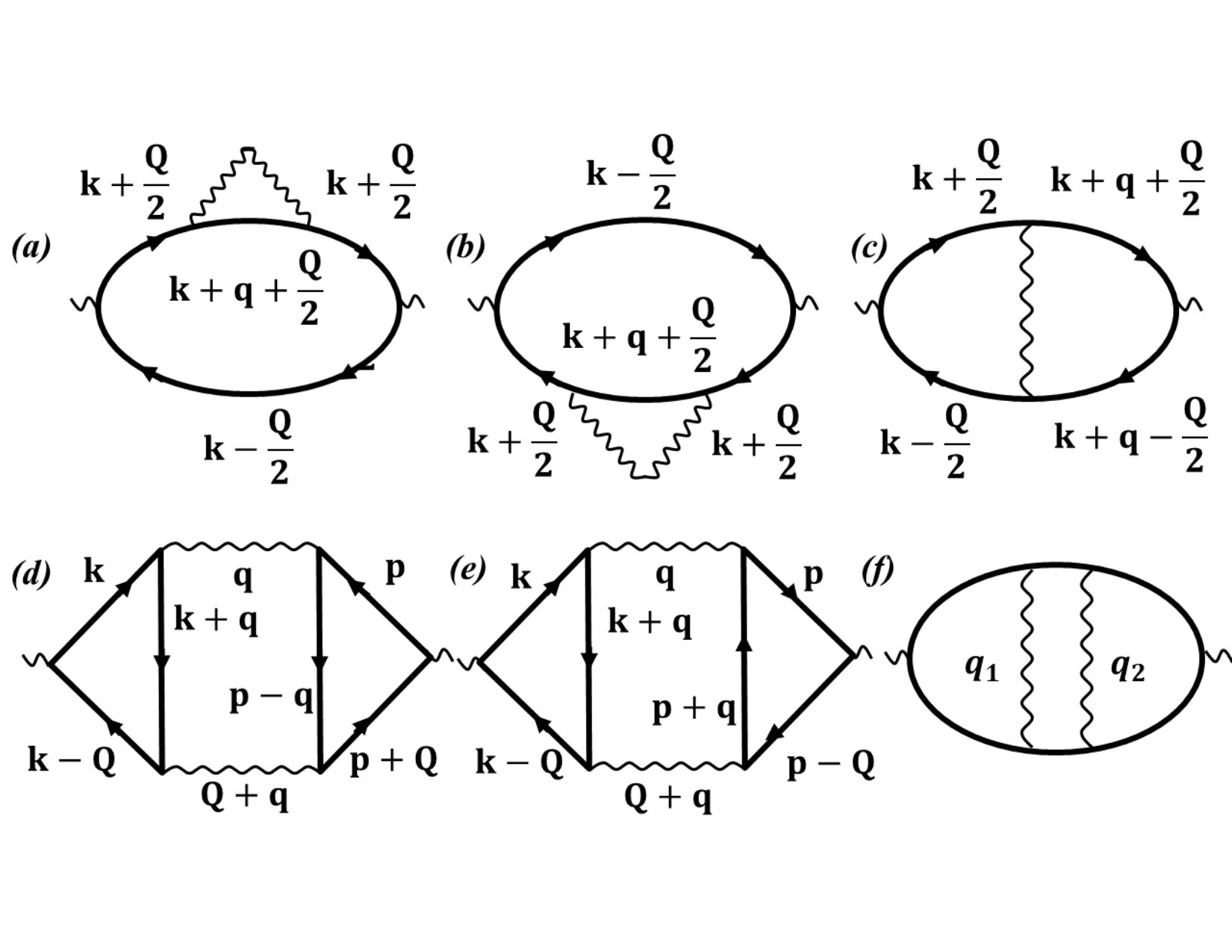 Figure 1
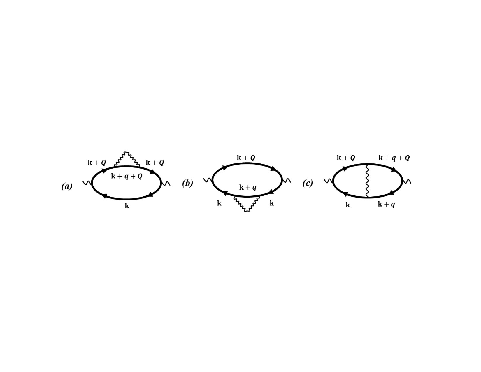 Figure 2
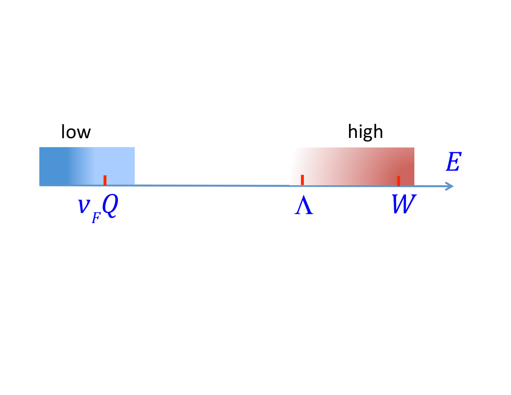 Figure 3
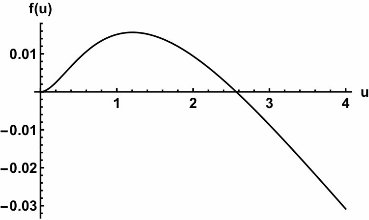 Figure 4
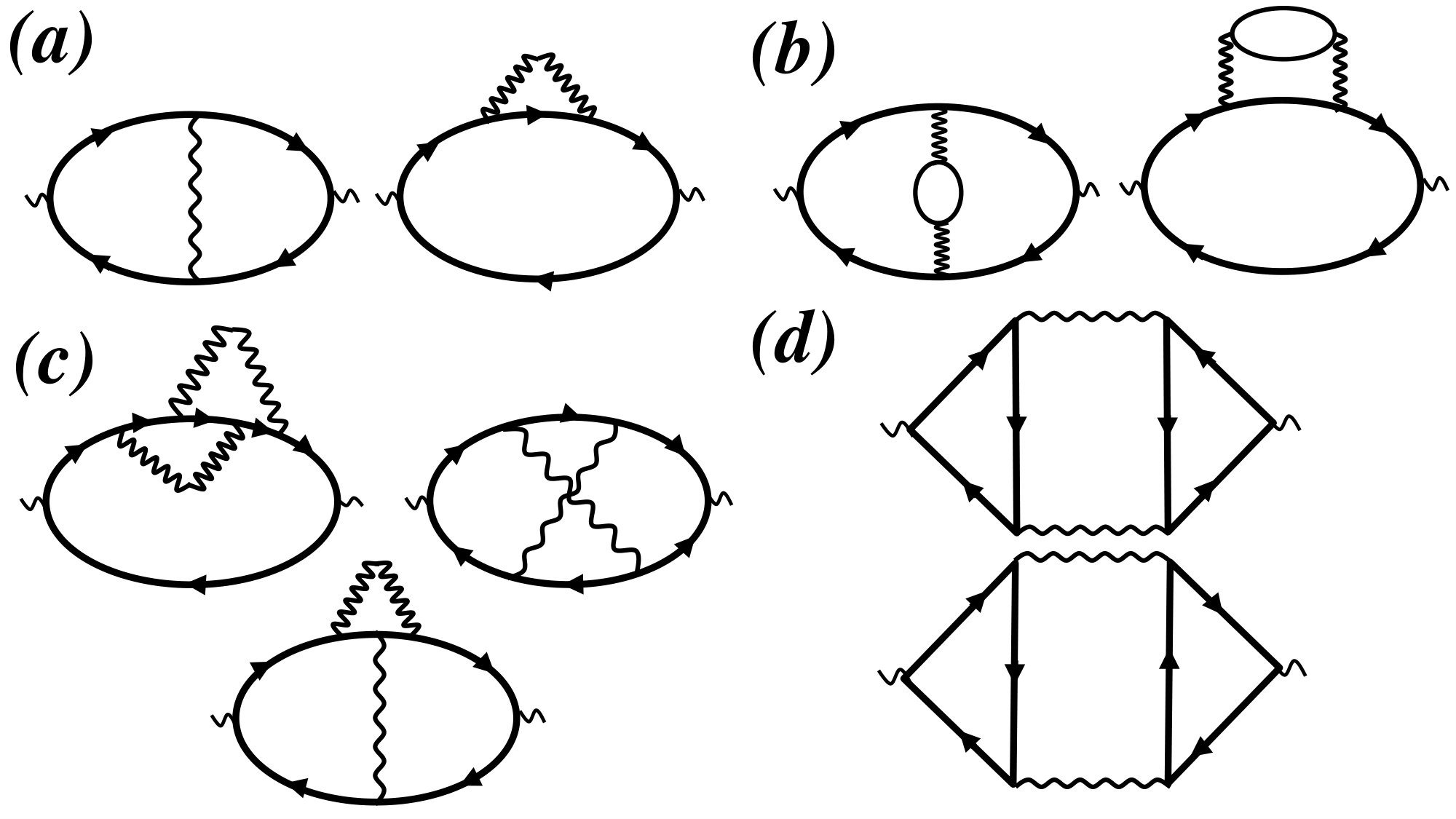 Figure 5
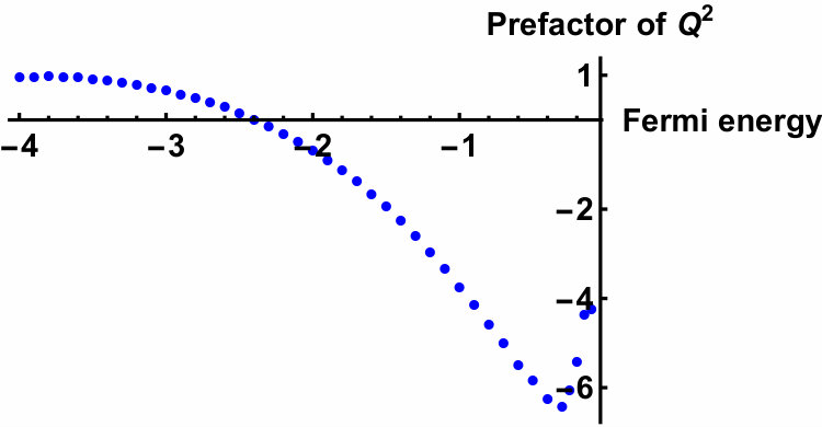 Figure 6
Peer Reviews
No public reviews on file for this paper yet. If you reviewed it on a platform where reviews are public (OpenReview, ICLR, NeurIPS, ICML), you can paste yours below so the community can read it here.
Videos
No videos yet. Explain this paper in a talk, walkthrough, or lecture? Add one.
Taxonomy
TopicsPhysics of Superconductivity and Magnetism · Quantum and electron transport phenomena · Cold Atom Physics and Bose-Einstein Condensates
Gradient terms in quantum-critical theories of itinerant fermions
Dmitrii L. Maslova,b, Prachi Sharmaa, Dmitrii Torbunovc, and Andrey V. Chubukovc
*a)*Department of Physics, University of Florida, Gainesville, FL 32611-8440, USA
*b)*National High Magnetic Field Laboratory, Tallahassee, Florida 32310, USA
*c)*Department of Physics, University of Minnesota, Minneapolis, MN 55455, USA
(March 3, 2024; March 3, 2024)
Abstract
We investigate the origin and renormalization of the gradient () term in the propagator of soft bosonic fluctuations in theories of itinerant fermions near a quantum critical point (QCP) with . A common belief is that (i) the term comes from fermions with high energies (roughly of order of the bandwidth) and, as such, should be included into the bare bosonic propagator of the effective low-energy model, and (ii) fluctuations within the low-energy model generate Landau damping of soft bosons, but affect the term only weakly. We argue that the situation is in fact more complex. First, we found that the high- and low-energy contributions to the term are of the same order. Second, we computed the high-energy contributions to the term in two microscopic models (a Fermi gas with Coulomb interaction and the Hubbard model) and found that in all cases these contributions are numerically much smaller than the low-energy ones, blue especially in 2D. This last result is relevant for the behavior of observables at low energies, because the low-energy part of the term is expected to flow when the effective mass diverges near QCP. If this term is the dominant one, its flow has to be computed self-consistently, which gives rise to a novel quantum-critical behavior. Following up on these results, we discuss two possible ways of formulating the theory of a QCP with .
I Introduction
Understanding the behavior of itinerant fermions near a quantum critical point (QCP) is crucial for describing correlated electron systems. The underlying idea is that near QCP the behavior becomes universal and can be described by a small number of exponents, which depend only on the type of symmetries broken in the ordered phase, and on spatial dimensionality.
QCP in a metallic system generally occurs at intermediate coupling, where the fermion-fermion interaction is of order of bandwidth . In this case, a perturbation theory in the original interaction is not a reliable computational scheme. A commonly accepted alternative Hertz (1976); Millis (1993); Moriya (1985); Abanov et al. (2003) is to abandon the underlying microscopic model and analyze instead an effective low-energy model of fermions interacting via the exchange of soft bosons that condense in the ordered state. Although such a model cannot, except for a few special cases, be derived in a controllable way from microscopics, it is generally believed to emerge once one integrates out fermions with energies between and some much smaller energy , which serves as the upper cutoff for the effective model (see Fig. 1). The anticipated universality of low-energy behavior implies that the behavior of observables at large distances and long time scales does not depend on a particular choice of , as long as .
The inputs for the low-energy model are the boson-fermion coupling and bare bosonic propagator, . The latter is a particle-hole polarization bubble, dressed by interactions involving fermions with energies between and . Fermions with such energies are assumed not to differ qualitatively from free one, even at QCP. As the consequence, the momentum and frequency dependences of are assumed to be regular, i.e., expandable in powers of and , where is the momentum at which bosons condense in the ordered phase. The regular frequency dependence of is often omitted in anticipation that renormalizations within the low-energy model produce a much stronger, non-analytic frequency dependence (Landau damping). This non-analytic dependence comes from fermions with energies , and it emerges regardless of whether the system is at QCP or away from it. With few exceptions (discussed later in this section),Belitz et al. (2005); Löhneysen et al. (2007); Brando et al. (2016) there is no analogous non-analytic contribution to the momentum dependence of the bosonic propagator, hence the dependence of on is essential and must be kept. In most theories, this dependence is taken to be of the Ornstein-Zernike form:
[TABLE]
where is of order of the static and uniform susceptibility of free fermions, is a model-dependent parameter, generally of order of the interatomic spacing, and (dimensionless) is the measure of the distance to QCP. Boson-fermion models with given by Eq. (1) have been studied extensively both for finite (a density-wave QCP) and (a ferromagnetic or nematic QCP, or the model of fermions interacting with a gauge field). When only the Landau-damping contribution from low-energy fermions is included, the critical bosonic propagator has dynamical exponent of for a finite- QCP [in this case, the prefactor of the Landau-damping term is a constant] and for a QCP [in this case, with ]. Beyond this approximation, the interaction between low-energy fermions and critical bosonic fluctuations gives rise to a singular frequency dependence of the fermionic self-energy in dimensions , leading to a non-Fermi liquid (NFL) behavior at QCP. In 2D (and in some specially crafted models in ) these singular renormalizations also give rise to anomalous exponents for fermionic and bosonic propagators, and may also change the value of the dynamical exponent .
In this paper, we discuss another aspect of the low-energy model, which attracted less attention until recently.Wölfle and Abrahams (2011); Abrahams et al. (2014) This new aspect is an observation that low-energy fermions can also contribute to the regular dependence of the bosonic propagator. This additional contribution is often neglected because it is assumed to be smaller than that from high-energy fermions by a factor of , simply because the energy width of the low-energy model is small (below we will dispute this assumption for the case). However, the parameter in the high-energy contribution [Eq. (1)] is model-dependent and, in principle, can be rather small. If we assume momentarily that this is the case and set in Eq. (1), we encounter a situation when the bare bosonic propagator is just a constant, and both the Landau-damping and gradient terms in come from low-energy fermions. Away from a QCP, it does not really matter whether the gradient terms come from high or low energies. Near a QCP, however, the low- and high-energy contributions are qualitatively different. Namely, the high-energy contribution is insensitive to NFL physics, specifically to the divergence of the effective mass. The contribution from low-energy fermions, on the other hand, depends on the effective mass. In Eliashberg-type theories, where the self-energy near a QCP depends predominantly on the frequency, the fermionic residue accounts for renormalization of the fermionic dispersion [, which means that the ratio of the effective and bare quasiparticle masses is . Then, if one keeps only the low-energy contribution to the gradient term, one ends up with a new theory in which mass renormalization has to be computed self-consistently with the bosonic dispersion. We emphasize that this holds even in cases when bosonic propagators do not acquire anomalous dimensions.
The spin-fermion model with an additional mass-dependent prefactor of the gradient term in the bosonic propagator has been recently put forward by Wolfle and AbrahamsWölfle and Abrahams (2011) in the context of an antiferromagnetic QCP in . In this case a high-energy contribution to the gradient term should also be present, and it is not a priori clear why it can be neglected, given that in a generic case this should be the largest contribution. At the same time, the analysis in Ref. Wölfle and Abrahams, 2011 and subsequent work Abrahams et al. (2014) demonstrated a very good agreement between this theory and the data for a number of heavy-fermion materials. This calls for further investigation of the interplay between high- and low-energy contributions to the gradient term in these systems.
In this paper, we study the case of , which is special for two reasons. First, we show that low-energy contribution to the is of the same order as high-energy contribution, i.e., it is not small in . Second, we show that the high-energy contribution to the term is absent if the interaction between high-energy fermions is approximated as static, and emerges only if one includes dynamical screening of this interaction.
To demonstrate these two features, we analyze the interplay between high- and low-energy gradient terms first within the random phase approximation (RPA), which neglects dynamical screening of the interaction by high-energy fermions, and then for two models with a dynamical interaction between high-energy fermions.
The first model is a Fermi gas with a dynamically screened Coulomb interaction. In principle, this model can be tuned to a critical point in the spin channel or in the charge channel with angular momentum . We will not analyze a specific path to quantum criticality, but rather compute the term in dressed bosonic propagators in the spin and charge channels. We show that the low-energy contribution to the term comes from fermions with energies of order of , where is the Fermi velocity, while the high-energy contribution comes from energies of order of the effective plasma frequency, . Our reasoning for the separation between the low- and high-energy contributions holds if , which in practical terms implies that the enhancement of the mass ratio is confined to energies below . We show that the (numerically) dominant contribution to the term comes from low-energy fermions both in 2D and 3D. The difference between the high- and low-energy contributions is particularly spectacular in 2D, where the high-energy contribution accounts only for two percent of the total. Moreover, we found that the sign of the high-energy part of the term is non-universal: it is negative in 2D and positive in 3D for fermions with a parabolic dispersion. For 2D fermions on a square lattice the high-energy part of the term changes sign near quarter-filling and stays positive all the way up to half-filling.
The second model is a Fermi gas with a parabolic dispersion and Hubbard interaction, which we set to be a constant () up to some momentum cutoff and then vanish. This model can be tuned to QCP in the spin channel (for positive ) or the charge channel (for negative ). We show that the high-energy contribution to the term emerges at second order in , once dynamical screening of the Hubbard interaction is included. As in the Coulomb case, we find that high-energy contribution to the term is numerically small. We extended the result beyond second order in by summing up RPA diagrams for screened interaction, and found that the prefactor of the high-energy term changes sign at some critical value of .
The outcome of our analysis is that the low-energy boson-fermion model for QCP with has to be reconsidered, at least in some cases. Namely, instead of starting from Eq. (1) for the bare propagator and neglecting additional contributions to from low-energy fermions, one has to set the bare propagator to be -independent and compute both the frequency and momentum dependences of within the low-energy model. The Landau-damping term does not depend on and is the same as for free fermions, but the prefactor of the term is reduced by critical fluctuations. As a consequence, the quantum-critical theory becomes qualitatively different from the one with the bare propagator given by Eq. (1).
We caution that, near QCP, our arguments apply to the behavior of the system at small but finite energies. At progressively smaller energies, the low-energy contribution to the term is reduced by growing and eventually gets smaller than the high-energy contribution, which is not affected by mass renormalization. As a result, the high-energy contribution dominates at the lowest energies, and the quantum-critical theory eventually becomes the ”conventional” one, if the high-energy term is positive. If it is negative, the system either develops an incommensurate order or the transition becomes first order. We emphasize that this is different from a first-order transition and an incommensurate magnetic order due to generation of a non-analytic momentum dependence of by an effective long-range interaction.Belitz et al. (2005); Löhneysen et al. (2007); Brando et al. (2016) The effect we consider here is related to a possible sign change of the analytic term. One difference is that the effect due to non-analyticity holds for an -symmetric ferromagnetic QCP, but is absent for a charge QCP and also if the symmetry is broken down to IsingChubukov et al. (2004); Rech et al. (2006) by, e.g., spin-orbit interaction.Żak et al. (2010, 2012) In contrast, the new physics, associated with potential negative sign of the term, holds for both spin and charge QCPs. Another difference is that a non-analytic -dependence of is a low-energy effect, while we are interested in a high-energy term.
The rest of the paper is organized as follows. In Sec. II we analyze the dressed bosonic propagator near within RPA and FL theory. In Sec. II.1 we show that the term in RPA comes exclusively from fermions with energies of order of , while the high-energy contribution is absent. In Sec. II.2 we include FL renormalizations on top of RPA. In Sec. III we compute both the low- and high-energy contributions to the term in the bosonic propagator for a model with dynamically screened Coulomb interaction. We show that the low-energy contribution still comes from energies of order of , while the high-energy one comes from energies of order of the effective plasma frequency. In Sec. IV we perform the same analysis for the Hubbard model. We discuss possible consequences of our results for low-energy theories of a QCP in Sec. V. Technical details of the calculations are given in Appendices A-C.
II
Bosonic propagator in RPA and in FL theory
II.1 RPA
To illustrate the issue with the gradient term in the bosonic propagator near the criticality, we first consider derivation of Eq. (1) within RPA for a system with a constant repulsive interaction . A system with sufficiently large repulsive is unstable towards ferromagnetism, and we focus on the spin susceptibility.
For free fermions, the static spin susceptibility , where is the free static polarization bubble (with an extra factor of two due to spin summation)
[TABLE]
where is the Green’s function and is the Matsubara frequency. The dressed spin susceptibility is given by a series of ladder diagrams, which is summed up into
[TABLE]
In the limit the polarization bubble is reduced to , where is the density of states at a Fermi level per two spin orientations. At finite , should in general have some regular dependence on , i.e., to be expandable in powers of :
[TABLE]
The prefactor vanishes in special cases, e.g., for 2D fermions with a parabolic or linear dispersion, but in general is non-zero. The issue we consider is where this term comes from.
The constant () term in Eq. (4) can be obtained in two ways – by integrating first over frequency and then over the momentum or vice versa.Maslov and Chubukov (2010) In the first method, one has to keep finite and set it to zero only at the end of calculation. The integral comes from the region where the poles of the integrand over in Eq. (2) are in the opposite half-planes. This imposes the conditions and (or vice versa) which, for , can be satisfied only for near the Fermi surface, when is at most comparable to . In our nomenclature, this implies that the integral comes from low energies. In the second method, one can set from the beginning but constraints integration over to the region . From Eq. (2) we then have
[TABLE]
This time, the integral comes from energies , i.e., from high energies in our nomenclature. The fact that the same result can be obtained in two ways implies that the term in the polarization operator for free fermions is an ”anomaly”,Treiman et al. (1972); Chubukov et al. (2008) which can be viewed as either as a low- or high-energy contribution, depending on the regularization procedure. This feature is a consequence of the double pole in the integrand of Eq. (4) for .
For the term, the situation is different. If we compute this term by the second method, i.e., by expanding the integrand in to order and integrate first over in finite limits and then over frequency, we get zero. This implies that there is no ”high-energy” contribution to for free fermions. If, on the other hand, we keep finite and integrate over frequency first, we do find a non-zero term. An explicit calculation for 3D fermions with an isotropic but otherwise arbitrary dispersion yields Maslov and Chubukov (2009)
[TABLE]
where , , and is the density of states as a function of energy. For a power-law dispersion, , we have . For a parabolic dispersion . A similar formula holds for the 2D case, the only difference is that in 2D both for parabolic and linear dispersions. The low-energy nature of this term is manifested by the fact that its prefactor is expressed entirely via the dispersion and its derivatives at the Fermi energy, i.e., comes from fermions with energies smaller than . In this respect, if we would construct the bare spin susceptibility for the effective low-energy model by integrating out fermions with energies much larger than , we would not obtain a term. At the same time, we see that the prefactor does not depend on the upper cutoff of the low-energy model and, hence, does not contain a small prefactor of . (Following along the same lines, we show in Appendix A that the diamagnetic susceptibility of a free electron gas, which is usually viewed as the property of the entire electron band, is in fact also a low-energy property in the sense defined above.)
II.2 Gradient term within the FL theory
The computational procedure in which the constant term in the polarization bubble comes from low-energy fermions can be extended in a rigorous way to include FL renormalizations. One way to to do this is to solve the kinetic equation for a FL in the presence of a magnetic field;A. A. Abrikosov, L. P. Gorkov, and I. E. Dzyaloshinski (1963); P. Nozières and D. Pines (1966); E. M. Lifshitz and L. P. Pitaevski (1980) another is to keep with diagrammatics,Finkel’stein (2010); Chubukov and Wölfle (2014) but to go beyond RPA and include self-energy and vertex corrections. Both procedures lead to the familiar result for the static and uniform spin susceptibility of a FL
[TABLE]
Within diagrammatics, this result comes about because self-energy corrections change the low-energy part of the Green’s function to , where , , and is the effective mass. The role of vertex corrections is to cancel the factors coming from the numerators of the Green’s functions. Also, the constant interaction is replaced by the zeroth harmonic of the Landau function in the spin channel FL via , where is the renormalized density of states at the Fermi level.
How FL renormalizations affect the term is a more difficult question, which, in general, has no definite answer in either the kinetic-equation or diagrammatic versions of the FL theory. Indeed, the FL theory operates with quasiparticles with dispersions linearized near the Fermi energy and thus contains only the first derivative of the dispersion (the Fermi velocity) but not higher derivatives, whereas one needs to know higher derivatives of the dispersion to obtain a term in the susceptibility [see Eq. (6)]. Keeping higher than terms in the dispersion is, strictly speaking, inconsistent with a FL assumption of non-decaying quasiparticles, because damping of quasiparticles occurs already at order .
One can approximately relate the prefactor of the term to the renormalized effective mass (which is a FL parameter) in the case of a local FL, when the self-energy depends on the frequency stronger than on the momentum. Such a case is realized near a QCP with (Refs. Chubukov, 2005; Metlitski and Sachdev, 2010a, b). In this situation, fermionic propagator can be approximated by , i.e., the whole fermionic dispersion acquires a factor . One can then re-calculate the term for free fermions with dispersion with an obvious result that in Eq. (6) is multiplied by . (The overall factor of in is canceled by vertex corrections.) Near a QCP, is supposed to diverge and thus the term vanishes. Therefore, mass renormalization changes the critical theory in a qualitative way compared to the case when the prefactor of the term is treated as a constant.
Although we said that the term, in general, cannot be obtained within the FL theory, it is still instructive to follow the consequences of including this term phenomenologically, as it is done, e.g., in some models of nematic instabilities.Oganesyan et al. (2001); Wu and Zhang (2004); Wu et al. (2007) Consider a special case of a FL, in which the interaction in the spin channel contains only the zeroth harmonic of the Landau function, . Solving a FL kinetic equation A. A. Abrikosov, L. P. Gorkov, and I. E. Dzyaloshinski (1963); P. Nozières and D. Pines (1966); E. M. Lifshitz and L. P. Pitaevski (1980) in the presence of a time- and position-dependent magnetic field, we obtain for the spin susceptibility
[TABLE]
where
[TABLE]
is the particle-hole polarization bubble in the small- limit, dressed by FL corrections, and denotes averaging over the angle between and . In the limit of , Eq. (8) is reduced to111It can be shown Zyuzin and Maslov that Eq. (10) is valid for an arbitrary Landau function with any number of harmonics but only in the limit .
[TABLE]
where is a numerical coefficient which depends on spatial dimensionality . Equation (10) does contain the bosonic mass (proportional to ) and the Landau-damping term but, as expected, it does not have a term. In this version of the FL theory, the term is absent because the quasi-classical kinetic equation contains only the first gradient of the distribution function, and thus enters only as .222This is also the reason why the FL theory does not have analog of Eq. (8) for the diamagnetic susceptibility, which is obtained as the prefactor of the term in the static current-current correlation function (see Appendix A). For an explicit calculation of the diamagnetic susceptibility renormalized by the Coulomb interaction, see Ref. Vignale et al., 1988 and references therein.
Suppose now that we “improve” the theory by adding a low-energy term term to the polarization bubble:
[TABLE]
(To ensure the ordering occurs at , we must also assume that .) Near criticality, when , the spin susceptibility then becomes
[TABLE]
with . We see again if the fermionic mass diverges near criticality while stays constant, the gradient term vanishes. This implies that the gradient term becomes a part of the low-energy theory and needs to be renormalized accordingly.
In the next two sections we show, on examples of two microscopic models, that there is a finite contribution to the term from high-energy fermions. Such contribution is not affected by by the divergence of the effective mass and hence survives at QCP. We found, however, that the high-energy contributions are numerically very small, at least in the models we considered. Therefore, at least over some range of energies, the dominant contribution to the term comes from low-energy fermions, and its prefactor does contain .
III Electron gas with Coulomb interaction
III.1 Formulation of the problem and background
We consider 2D and 3D electron gases with Coulomb interaction in the high-density limit. As we have already said in Sec. I, a term in the free-electron polarization bubble, , if non-zero, comes only from low energies. A term in the bubble, renormalized by the dynamically screened Coulomb interaction, was calculated in a seminal 1968 paper by Ma and Brueckner for a 3D electron gas. Ma and Brueckner (1968) Since then, the -dependence has been addressed by a large number of authors by semi-analytic or numerical means, see, e.g., Refs. Geldart and Taylor, 1970; Rajagopal, 1977; Maldague, 1978; Khalil et al., 2002. The difference between our calculation and the previous ones is that the goal of the latter was to obtain the entire term, which contains both low- and high-energy parts. On the other hand, we are interested only in the high-energy part of the term and will arrange the calculation in such a way that it picks up only that part. Comparison with prior work will allow us estimate the relative fraction of the high-energy part.
The minimum set of diagrams for the renormalized static polarization bubble, , is shown in Fig. 2 a-e. The interaction correction to the spin susceptibility is given directly by diagrams a-c. [The Aslamazov-Larkin diagrams d and e (or the fluctuation diagrams in the terminology of Ref. Ma and Brueckner, 1968) do not contribute, because the traces over Pauli matrices at the vertices vanish in the spin case by SU(2) symmetry.] On the other hand, the starting point for the charge susceptibility is the RPA formula , where is the bare Coulomb potential. To obtain beyond RPA, one simply needs to replace the bare polarization bubble in this formula by the renormalized one, which now includes the contributions of all five diagrams, a-e. The wavy lines in Fig. 2 correspond to the Coulomb potential, dynamically screened by free electrons
[TABLE]
where and are the screening momenta in , correspondingly. To keep the perturbation theory under control, we assume that (the high-density approximation) or, equivalently, that . Because typical momentum transfers are expected to be of order , the polarization bubble of free fermions in Eq. (13) can be approximated by its small limit:
[TABLE]
in and , correspondingly. 333By the same argument of small momentum transfers, the non-analytic, terms in the spin susceptibility, Belitz et al. (1997); Chubukov and Maslov (2003) which come from scattering processes, appear only at the next order in and can be neglected.
If the dynamic interaction is replaced by the static one, , the term in comes only from low-energy fermions. For example, diagram c in Fig. 2 in this case contain a product of two blocks
[TABLE]
where . Because the interaction is static, integrals over and in Eq. (16) are independent, and each of them confines the fermionic momenta and to narrow regions of width near the Fermi surface, i.e., only fermions with energies smaller that contribute. This calculation also shows that a low-energy term could not be obtained by Taylor-expanding Eq. (16) to order . Indeed, such an expansion would generate terms of order or higher, which vanish because the poles of the integrand are in the same half-plane of a complex variable . On the contrary, a high-energy term can be obtained via a straightforward Taylor expansion. On a technical level, this is the main difference between the low- and high energy gradient terms.
The -dependence of the susceptibility arising from the static Coulomb potential (the Hartree-Fock approximation) was calculated numerically in Ref. Geldart and Taylor, 1970 for and Ref. Maldague, 1978 for , and by a variational method for in Ref. Rajagopal, 1977. The low-energy contribution to the term for the static Coulomb potential in discussed in Sec. III.5 and Appendix C. The high-energy contributions to diagrams a-e can be singled out by subtracting off the static contributions, which amounts to replacing the Coulomb potential by its dynamic part
[TABLE]
This is the effective interaction that we will be using in the next section.
III.2 Spin
channel
The corrections to the polarization bubble in the spin channel, are given by diagrams a-c in Fig. 2. The calculations for and are very similar, and we present them in parallel. The self-energy diagrams a and b are equal. Labeling them as shown in Fig. 2, we obtain for their combined contribution
[TABLE]
while diagram c gives
[TABLE]
where and . For a quadratic spectrum , the dispersions in Eqs. (18) and (19) are expanded as
[TABLE]
Performing corresponding expansions in the Green’s functions and keeping only terms of order , we find that the high-energy term in consists of four parts
[TABLE]
where
[TABLE]
with
[TABLE]
It can be readily shown that
[TABLE]
Applying this identity to Eqs. (22a) and (22b), we find that all terms in square brackets cancel each other, and thus This result can be related to the fact that any two-particle correlation function is a gauge-invariant object and, as such, can contain the interaction potential only multiplied by factor that vanishes at .Zala et al. (2001) Such a factor ensures that there is no contribution from a potential which is constant in real space, i.e., a delta-function in the momentum space. There are no such factors in and , and therefore they must vanish.
The combination of the Green’s functions in square brackets in does not vanish on applying Eq. (24). This can be related to the fact the integrand contains a common factor of , and thus does not have to vanish identically. However, it still gives no contribution to leading order in . Indeed, integrating first over and approximating with , we find that each term in square brackets in Eq. (22c) yields a combination
[TABLE]
which is odd in . Since the potential is even in , the integral over vanishes, and thus to leading order.
The only term that does not vanish by gauge invariance and is non-zero to leading order is thus . (In Appendix B, we demonstrate another way of arriving at the same result by first combining diagrams Fig. 2 a-c and then expanding the result to order .) The calculation of is fairly straightforward. The frequency integrals in are calculated as
[TABLE]
where and . Now we replace by , where is the solid angle in dimensions, and integrate over . The integral over is confined by the sign functions in Eq. (26) to the region and gives a factor of . Averaging over the angle between and (the direction of which is chosen as a reference) yields
[TABLE]
where
[TABLE]
Finally, averaging over the angle between and gives a factor of . After these manipulations, we obtain
[TABLE]
Now it is convenient to introduce dimensionless variables and . In , the integrals over and can be solved analytically:
[TABLE]
In , the integral over is solved analytically but the integral over needs to be solved numerically, which yields
[TABLE]
As we mentioned before, Eqs. (III.2) and (31) give directly the term in the spin susceptibility: .
Tracing back our steps, we note that all the internal energy scales are of order of effective plasma frequency : . Therefore, the terms in Eqs. (III.2) and (31) are indeed of the high-energy type.
For typical values of and , the dynamically screened potential in Eq. (13) is of order of and does not depend on the electric charge. Although higher-order diagrams contain higher powers of the interaction, the interaction is not small in the dimensionless coupling constant of the theory, . This may raise a concern about convergence of the perturbation theory. Fortunately, this concern is not legitimate, as higher-order diagrams have more integrals over internal energy scales, which do bring additional factors of compared to lowest-order diagrams a-c. To see this, one can compare, e.g., diagram c with a next-order diagram, e.g., diagram f. The main contribution to diagram c comes from expanding the fermionic dispersion to order , and then expanding the corresponding Green’s function to second order in this parameter, which is equivalent to replacing one of the four Green’s functions in this diagram by . Consequently, the term from diagram c contains six Green’s functions, and by power-counting . Integrals over , , , and altogether give a factor of , and another comes from in the expansion of dispersion. Overall, the count is both in and . Now, assuming that the main contribution to diagram f also comes from terms of order in the dispersions, we end up with eight Green’s functions . The number of the fermionic variables remains the same but the number of bosonic ones is doubled, therefore integrations give . With an extra factor of from either or , the overall count of diagram f is , which is smaller than diagram c by a factor of .
III.3 Charge
channel
In addition to the contribution from diagrams a-c in Fig. 2, the polarization bubble in the charge channel also contains the contribution from Aslamazov-Larkin diagrams d and e. It will be shown in this section, however, that the high-energy terms from diagrams d and e cancel each other, so Eqs. (III.2) and (31) apply to the charge channel as well.
Labeling the diagrams as shown in Fig. 2, we obtain for the sum of diagrams d and e:
[TABLE]
The dispersions are expanded to order as . We will also need to expand the interaction, which depends on the magnitude of , as
[TABLE]
where , , and is the angle between and .
It is convenient to split into two parts. The first part () contains all but the terms arising from the terms in the expanded dispersions, while the second part () contains the remaining terms. Collecting all terms in , we obtain
[TABLE]
where shorthands for with are the same as in Eq. (23), , and
[TABLE]
Now let’s define
[TABLE]
where . On expanding , it can be readily seen that . Therefore
[TABLE]
for any , and thus .
Next, we collect terms and obtain
[TABLE]
The term with vanishes as before by Eq. (37). In the second term, one needs to go one step farther. Integrating the combination over and , we obtain (up to an inessential prefactor)
[TABLE]
Likewise, integration of the product over and yields
[TABLE]
The product of Eqs. (39) and (40) is odd under a simultaneous change and , whereas is even. Hence the integral of the second term in Eq. (38) vanishes as well, which means that =0. Therefore, the contribution from the Aslamazov-Larkin diagrams vanishes, i.e., the high-energy term in the polarization bubble in the charge channel is the same as in the spin channel
[TABLE]
III.4 2D case, lattice dispersion
The sign of the high-energy gradient term in 2D [Eq. (III.2)] is positive. If the low-energy term is reduced by critical fluctuations, i.e., by a factor of , then it is the high-energy term that determines the behavior of near QCP. The positive sign of this term would indicate that the susceptibility is peaked at finite , and thus a QCP is pre-empted by a finite- instability. However, the positive sign was obtained for a special case of fermions with a quadratic spectrum, and its universality needs to be verified. Obviously, the sign will remain the same for any isotropic but not necessarily quadratic dispersion: in this case one just needs to replace a factor of in Eq. (22d) by the inverse effective mass . To check whether the sign can be reversed in the presence of a lattice, we computed numerically the prefactor of the high-energy gradient term in the same model with a long-range Coulomb interaction but for electrons on a square lattice with a tight-binding dispersion . 444Strictly speaking, the interaction of electrons on a lattice must be described by matrix elements of the bare Coulomb potential in the basis of Wannier functions. This changes the magnitude of the Coulomb potential but not its form. As we are interested here only in the sign of the effect, we ignore this complication and use the same bare Coulomb potential as for electrons in continuum. The dynamically screened Coulomb interaction is the same as in Eq. (13), except for now is the polarization bubble of electrons on a square lattice, which we computed numerically for a range of filling factors. The calculation follows the same lines as in Sec. III.2. We focus on the leading contribution to the term [ in Eq. (22d)], calculate the integrals over and analytically, and compute the remaining four-dimensional integral over , , and along the Fermi surface numerically. By symmetry, the term is isotropic. In Fig. 3, we plot its prefactor as a function of the Fermi energy, measured in units of , such that corresponds to the bottom of the band. For , the numerical solution reproduces the analytic result in Eq. (III.2) with high accuracy. However, at larger fillings, we found a new behavior. Namely, Fig. 3 shows that the prefactor of the term changes sign around quarter-filling () and remains negative all the way up to half-filling (). A negative prefactor for implies that has a maximum at , as expected near QCP towards an order with . We see therefore that lattice tends to stabilize a QCP, given that the maximum of at is higher than that at finite .
III.5 Relative magnitudes of high-energy and low-energy contributions to
the term
We found in previous sections that the magnitude of the prefactor of the high-energy term, in units of , happens to be numerically small both in 2D and 3D. This naturally raises a question about the ratio of high-energy to low-energy parts of the term.
In 3D, the low-energy contribution is non-zero already for free fermions, whereas the high-energy contribution comes only from interaction and is therefore parametrically small at small . The interaction correction to the low-energy part is small as well. For , all contributions to become of the same order, and it makes sense to compare the numerical prefactors. The same set of diagrams as in Fig. 2 for the polarization bubble was computed numerically in Ref. Khalil et al., 2002 for . We digitized the data of Ref. Khalil et al., 2002, fitted the small- parts of the curves by a form, and extracted the total interaction-dependent prefactor of the term, which contains both low- and high-energy contributions. Comparing the total numerical prefactor with the analytic result for the high-energy contribution, given by Eq. (31), we found that the high-energy contribution amounts to about and of the total for the charge and spin susceptibilities, correspondingly. 555Reference Khalil et al., 2002 gives the results for diagrams a-c and d-e separately, from which one can extract the polarization bubbles both in the charge and spin channels. At the same time, the total interaction-induced term in the spin and charge susceptibilities for is about and of the free-fermion result, correspondingly.
The 2D case is different in that the free-fermion polarization bubble for fermions with a parabolic dispersion is independent of up to , i.e., the prefactor of the term is zero. This degeneracy can be broken by lattice but, at low enough filling, the term in the free-fermion bubble is still small. Then both high- and low-energy contributions to the term come from interaction, which allows for a direct comparison between the two contributions. In what follows we focus on the spin susceptibility. We estimated the low-energy contribution to the interaction-induced term by evaluating the diagrams in Fig. 2(a-c) with a statically screened Coulomb potential, . (In Sec. III.2 we subtracted off this contribution.) We obtained (see Appendix C for details):
[TABLE]
where in 2D.
The -dependence of the polarization bubble in 2D due to static Coulomb interaction was addressed in Refs. Rajagopal, 1977 and Maldague, 1978. There is some confusion about the results in prior literature which needs to be clarified. Namely, the numerical calculation in Ref. Maldague, 1978 was performed for the bare Coulomb potential () and produced a finite result for the susceptibility at all , whereas in Ref. Rajagopal, 1977 it was argued that the prefactor of the term is divergent at . Actually, these two results do not contradict each other. We found, in agreement with Ref. Rajagopal, 1977, that the leading term in the dependence of for the bare Coulomb potential is rather than . If screening is taken into account, is replaced by , as it is the case in Eq. (LABEL:low). At the same time, we see that the numerical prefactor of the term in Eq. (LABEL:low) is much smaller (by a factor of ) than that of the term, so the numerical results of Ref. Maldague, 1978 are indeed well-described by the form except for the region of extremely small .
The -dependence of the polarization bubble in 2D due to the dynamically screened Coulomb interaction was also calculated numerically in Ref. Khalil et al., 2002. Fitting the result of Ref. Khalil et al., 2002 for the spin susceptibility into a form at , we found that it is described by Eq. (LABEL:low) very well. This implies that the interaction-induced term comes primarily from low energies. Comparing the numerical result for the total interaction-induced term with our analytic result for its high-energy part [Eq. (III.2)], we found that the latter amounts to about of the former. (For the charge channel, the fraction of the high-energy part is about .)
Another comment on the 2D case is in order. That the susceptibility of non-interacting electrons with quadratic dispersion is flat up to indicates a high degree of frustration with respect to ordering into a state with finite . (The same flatness holds for 2D fermions with a Dirac dispersion. Kotov et al. (2012)) The Coulomb interaction lifts this degeneracy, and numerical calculations show that the full susceptibility is peaked at .Maldague (1978); Khalil et al. (2002) (Note in this regard that the prefactors of the terms in Eqs. (III.2) and (LABEL:low) are positive, i.e., the susceptibility increases with increasing .) For electrons on lattice, the tendency to ordering at finite rather than zero is pronounced already in the non-interacting case: numerical calculations for square, triangular, and honeycomb lattices show that the susceptibility is peaked at the momenta connecting certain points on the FS.Wang et al. (2016); Ozawa et al. (2016); Batista In light of these results, a 2D electron system may not seem to be a good candidate for a instability. Nevertheless, the type of an instability in an interacting system is decided by the relative strengths of renormalizations of at and finite . The former is determined by FL parameters, while the latter cannot be quantified in this way and depends on details of the electron spectrum and interaction. Even though of free electrons may have a peak at finite , the peak in renormalized may be higher, and thus the instability may win. In addition, the Kohn anomaly, which leads to a peak at , is weakened under certain circumstances, e.g., in chiral electron systems, such as graphene and surface states of 3D topological insulators, due to suppression of backscattering into states with opposite (pseudo) spins.Kotov et al. (2012)
IV
A term in the Hubbard model
As another example, we compute the polarization bubble of interacting fermions assuming that the four-fermion interaction is Hubbard-like, i.e., it is equal to a constant for below some cutoff, , and is zero for larger . To simplify calculations, we set to be much smaller tan . This will allow us to use a small- and small- form of the polarization bubble, Eq. (14).
To first order in (panel a in Fig. 4), the self-energy diagram amounts to shifting the chemical potential, while the vertex diagram is reduced to a product of two free-fermion polarization bubbles. None of the above produces a high-energy term. However, the situation changes at second order in because now self-energy and vertex renormalizations within a particle-hole bubble can be viewed as dynamical screening of the interaction between high-energy fermions. In this respect, the Hubbard model, taken at order , becomes similar to the model with dynamically screened Coulomb interaction, taken at first order in this interaction. It remains to be seen, however, whether the prefactor of the term in the Hubbard model is of the same sign and comparable magnitude as for the model with Coulomb interaction. Interaction-induced corrections to the static polarization bubble in the Hubbard model were analyzed in Ref. Chubukov, 1993 without making a distinction between low-energy and high-energy contributions. Our goal is to distinguish between the two.
There are seven distinct non-RPA diagrams for renormalization of to second order in , which potentially can give rise to a high-energy term. We show them in panels b-d of Fig. 4. Five of these diagrams, shown in panels b and c, renormalize both the charge and spin susceptibilities, while the Aslamazov-Larkin diagrams, shown in panel d, renormalize only the charge susceptibility.
For definiteness, we consider 2D case and approximate the fermionic dispersion by a parabolic one. We found that the three diagrams in panel c and two Aslamazov-Larkin diagrams in panel d are smaller in than the two diagrams in panel b. The two last diagrams can be viewed as vertex and self-energy corrections to the particle-hole bubble coming from effective interaction . To explore the region of somewhat larger , we will extend this formula to the full RPA result . The actual diagrams that need to be evaluated are then the first-order diagrams (panel a) in which is replaced by . The second-order result can be obtained by expanding the effective interaction back to second order in . Expanding these diagrams to order , and integrating over fermionic frequencies and momenta in the same way as in Sec. III, we obtain for the high-energy contribution to the polarization bubble in the spin channel
[TABLE]
where
[TABLE]
and
[TABLE]
Here, and is given by Eq. (28a). One can check that the remaining integral over vanishes if the effective interaction is approximated as static, i.e., the last factor in the integrand of Eq. (LABEL:n_5) is replaced by . We follow the same strategy as in Sec. III and just subtract off the static interaction from Eq. (LABEL:n_5). Then the delta-function term in Eq. (LABEL:n_5) can be omitted, and the expression for becomes
[TABLE]
This expression is similar to the corresponding formula for Coulomb interaction in 2D [Eq. (29)] with one important distinction. For the Coulomb case, the interaction behaves as and, as a consequence, the integral over in Eq. (29) is ultraviolet convergent, i.e., integration over can be extended to infinity. For the Hubbard case, the integral over in Eq. (46) is not convergent and needs to be cut off at .
Substituting Eq. (46) into Eq. (44), we obtain
[TABLE]
where
[TABLE]
At small ,
[TABLE]
We see that, at weak coupling, the prefactor of the term in is positive. As the consequence, imcreases with increasing . This is similar to what we obtained for the Coulomb interaction in 2D for a parabolic dispersion. Also, as in the Coulomb case, the magnitude of the high-energy contribution to the term is numerically very small.
Function in plotted Fig. 5. We see that the magnitude of remains small for all , but changes sign at and becomes negative for larger . At such , becomes a decreasing function of , i.e., has at least a local maximum at .
We note, however, that the prefactor of the term changes its sign at a rather large . Whether at such the system still does not order magnetically is unclear (within RPA, the Stoner instability occurs at , but the value of changes due to corrections beyond RPA).
A low-energy contribution to the term in in a 2D system with a parabolic dispersion also emerges to second order in . A computation of this contribution is rather involved and we left it aside. We note, however, that the low-energy contribution is non-zero already for free fermions, once we include higher powers of into an isotropic dispersion or put the model on a lattice.
V Discussion and conclusions
We now discuss the results of the previous sections in the context of a quantum-critical theory. We have shown that there are two contributions to the gradient () term in the bosonic propagator near a QCP. One comes from fermions with high energies, by which we understand energies above the upper cutoff of the effective boson-fermion low-energy theory, . Another comes from fermions with low energies, of order of . The low-energy contribution is present already in the bosonic susceptibility made of free fermions (except for the special cases of, e.g., linear and parabolic dispersions in 2D). To get a high-energy contribution to the term, one has to include dynamical screening of the interaction between high-energy fermions. If only static screening is included, the high-energy contribution is absent.
The low-energy part of the term near a QCP is not reduced by a small ratio of to the fermionic bandwidth. However, it is reduced near QCP by a divergence in the effective mass . There is no general formula relating the prefactor of the low-energy term to the Landau parameters. However, if near QCP the fermionic self-energy depends on the frequency much stronger than on the momentum, the low-energy part of the term is reduced by a factor of . The high-energy contribution to term is not reduced by and, in general, has to be the dominant contribution near QCP.
We found, however, that, at least in two microscopic models, the high-energy contribution to the term is numerically very small. The most spectacular example is a 2D Fermi gas with Coulomb interaction – the high-energy contribution to term in the bosonic susceptibility is less than two percent of the total.
Based on these numbers, one can envisage two possible types of quantum-critical theories. In the first one, adopted in earlier studies, the numerical smallness of the high-energy terms is disregarded as an artifact of a particular model. The starting point for such a theory is a high-energy action with a term, which is not assumed to be small. Such a theory has dynamical exponent and yields the fermionic self-energy , modulo logarithmic corrections.Metlitski and Sachdev (2010a, b) In the second type of theories, the smallness of the high-energy term is treated as the real effect, and the bosonic propagator at energies is taken to be independent of , at least to first approximation. Then the entire term in the bosonic propagator comes from low energies, and its prefactor depends on . Because in critical boson-fermion theories the fermionic self-energy, and hence , depends on the prefactor of the term, one now has to solve for self-consistently, keeping in the prefactor of the term. Such a procedure has not been yet implemented for the critical behavior near a QCP.
The self-consistent procedure of this kind was implemented in Refs. Wölfle and Abrahams, 2011; Abrahams et al., 2014 for an antiferromagnetic QCP (an instability at ). In this theory, the prefactor of the term in the bosonic propagator is set phenomenologically to scale as , and the consequences of this choice for the quantum-critical behavior are analyzed. At finite , the high-energy contribution to the gradient term is non-zero already for free fermions, and in general it is not small. At the same time, the low-energy contribution is reduced by a factor of . Then, in a generic case, the largest contribution to the gradient term should come from high energies, as it is assumed in conventional boson-fermion theories near a QCP.Abanov et al. (2003) However, in light of our results for the case, it would be interesting to analyze the high-energy terms in a broader set of models.
Acknowledgements.
We thank N. Prokofiev for his help with the numerical calculation, and E. Abrahams, C. Batista, S. Maiti, P. Wolfle, and V. A. Zyuzin for stimulating discussions. P.S. acknowledges support from the Institute for Fundamental Theory, University of Florida. The work of A.V.C. was supported by the NSF via grant DMR-1523036.
Appendix A Diamagnetic susceptibility as a low-energy property
It is commonly assumed that the diamagnetic susceptibility of a free Fermi gas, , is determined by all occupied states, both far below and near the Fermi energy.Levitov and Shytov ; Tsvelik (1995) In our terminology, this makes a high-energy property. This argument is based on the thermodynamic way of calculating ,Landau and Lifshitz (1980) in whihc one first finds the Landau levels, then calculates the free energy as a sum over these levels, and finally differentiates the result over the magnetic field. Such a procedure can be carried out only in those cases when the exact form of the Landau spectrum is known, e.g., for parabolic and linear dispersions. However, one can also calculate within the linear-response theory,Hebborn and March (1970); Levitov and Shytov ; Tsvelik (1995) as a prefactor of the term in the current-current correlation function. The result of such a calculation, Eq. (53), which can be carried out for an arbitrary electron dispersion, is similar to that for the prefactor of the term in the charge or spin susceptibilities [Eq. (6)] in that is entirely parameterized by the derivatives of the dispersion at the Fermi energy. This implies that is, in a fact, a low-energy property. Some details of the calculation are presented below.
As in Ref. Maslov and Chubukov, 2009, we assume that the electron dispersion is an isotropic but otherwise arbitrary function of . With chosen as the -axis, we need to calculate the term in the component of the current-current correlation function
[TABLE]
where . Defining , the diamagnetic susceptibility is found as . Summation over gives
[TABLE]
where is the Fermi function. Next, we expand the dispersion, the -component of the velocity, and the Fermi function to order as
[TABLE]
Here, are the polar and azimuthal angles of , , is the group velocity, is the effective mass, and . For a parabolic spectrum, , , , and is independent of . At , the derivatives of the Fermi functions are replaced by . Subtracting off the -independent term from , integrating over by parts, and averaging over the angles, we arrive at the final result for the diamagnetic susceptibility:
[TABLE]
For a parabolic dispersion, the last equation is reduced to
[TABLE]
as it should.
Appendix B A manifestly gauge-invariant way of collecting diagrams
In this Appendix, we show how diagrams a-c in Fig. 2 can be combined in a manifestly gauge-invariant way. For convenience, we relabel the diagrams as shown in Fig. 6 and adopt “relativistic” notations: , , and . will be set to zero later on in the calculation.
The sum of the self-energy diagrams (a and b) can be written as
[TABLE]
where
[TABLE]
is the one-loop self-energy.
Re-writing the product of the Green’s functions as
[TABLE]
we represent as a sum of two parts , where
[TABLE]
Now we restrict to the case of small momentum transfers, which is relevant for the Coulomb interaction. In this case, the dispersion of the Green’s function in Eq. (56) can be expanded as . The integral of over and gives, up to a prefactor,
[TABLE]
The second factor in the last formula in Eq. (59) is odd upon and , while is even, and therefore .
Applying Eq. (57) again and using an explicit form of , we obtain for the remaining part of :
[TABLE]
Applying Eq. (57) to diagram c in Fig. 6, we obtain
[TABLE]
Combining the self-energy and exchange contributions, we arrive at the following result for the spin susceptibility
[TABLE]
where
[TABLE]
By spin conservation, the spin susceptibility must vanish at and finite . Equation (62) satisfies this condition because the numerator of in Eq. (63) vanishes at . After this check, we set upon which is reduced to
[TABLE]
It is clear that vanishes at finite and , which guarantees the gauge invariance of the result.
Expanding the integrand in Eq. (62) to order , one obtains parts and of the spin susceptibility, given by Eqs. (22c) and (22d). Parts and are absent in this approach as their integrands do not contain factors of and thus vanish identically by gauge invariance.
Appendix C A term in the polarization bubble for the static Coulomb potential
In this Appendix we present details of the calculation of the term in the polarization bubble for the static Coulomb potential. As discussed in Sec. III.5, this is a low-energy contribution, arising from fermions with energies of order of .
To lowest order in the interaction, the susceptibility is given by the sum of three diagrams in Fig. 6, where now the wavy line corresponds to a statically screened Coulomb potential; in 2D, . In Appendix B, we showed how to combine these diagrams in a manifestly gauge-invariant way. The result is presented in Eq. (62) with in the static case given by Eq. (64). Following Ref. Geldart and Taylor, 1970, we symmetrize the result by relabeling , splitting it into two equal parts, and interchanging in one of the parts. Summing also over frequencies and , and expanding , we obtain
[TABLE]
The purpose of symmetrization was to make the suppression of the singularity in the Coulomb potential at more prominent: indeed, now the factor in square brackets vanishes at . However, the singularity is not removed completely: in the absence of screening (), the prefactor of the term still diverges logarithmically.Rajagopal (1977)
Next, we expand the Fermi functions to third order in and , and collect all terms of order . This gives , where
[TABLE]
The singularity at in the second line of the above equation is removed by considering the integral in the principal value sense.
At , the derivatives of the Fermi functions are reduced to the delta-function and its derivatives, after which it is easy to integrate over and by parts. In what follows, we will need expansions of all factors in the integrand up to . These are given by
[TABLE]
where and . Integrating by parts over and in Eq. (66), we obtain
[TABLE]
The angular integrals in the equations above are expressed through the angular harmonics of the following functions
[TABLE]
This gives
[TABLE]
At weak coupling (), the harmonics entering the equations above need to be determined to order . A straightforward computation yields
[TABLE]
Substituting Eq. (71) into Eq. (70), we obtain Eq. (LABEL:low) of the main text.
The reference list from the paper itself. Each links out to its DOI / PubMed record.
- 1Hertz (1976) J. A. Hertz, Phys. Rev. B 14 , 1165 (1976) . · doi ↗
- 2Millis (1993) A. J. Millis, Phys. Rev. B 48 , 7183 (1993) . · doi ↗
- 3Moriya (1985) T. Moriya, Spin Fluctuations in Itinerant Electron Magnetism (Springer Berlin, 1985).
- 4Abanov et al. (2003) A. Abanov, A. V. Chubukov, and J. Schmalian, Adv. Phys. 52 , 119 (2003) . · doi ↗
- 5Belitz et al. (2005) D. Belitz, T. R. Kirkpatrick, and T. Vojta, Rev. Mod. Phys. 77 , 579 ((2005).) . · doi ↗
- 6Löhneysen et al. (2007) H. V. Löhneysen, A. Rosch, M. Vojta, and P. Wölfle, Revi. Mod. Phys. 79 , 1015 (2007) . · doi ↗
- 7Brando et al. (2016) M. Brando, D. Belitz, F. M. Grosche, and T. R. Kirkpatrick, Rev. Mod. Phys. 88 , 025006 (2016) . · doi ↗
- 8Wölfle and Abrahams (2011) P. Wölfle and E. Abrahams, Phys. Rev. B 84 , 041101 (2011) . · doi ↗