Integral equation formulation of the biharmonic Dirichlet problem
Manas Rachh, Travis Askham

TL;DR
This paper introduces a new integral representation for solving the biharmonic Dirichlet problem, improving robustness and accuracy, especially on high-curvature domains, by leveraging a connection to Stokes flow.
Contribution
The authors develop a novel integral formulation for the biharmonic Dirichlet problem using a Stokes problem analogy, applicable to complex domains, enhancing computational stability.
Findings
New integral representation with better kernel behavior on high-curvature domains
Augmentation techniques for handling simply and multiply connected domains
Numerical examples demonstrating improved robustness and accuracy
Abstract
We present a novel integral representation for the biharmonic Dirichlet problem. To obtain the representation, the Dirichlet problem is first converted into a related Stokes problem for which the Sherman-Lauricella integral representation can be used. Not all potentials for the Dirichlet problem correspond to a potential for Stokes flow, and vice-versa, but we show that the integral representation can be augmented and modified to handle either simply or multiply connected domains. The resulting integral representation has a kernel which behaves better on domains with high curvature than existing representations. Thus, this representation results in more robust computational methods for the solution of the Dirichlet problem of the biharmonic equation and we demonstrate this with several numerical examples.
Click any figure to enlarge with its caption.
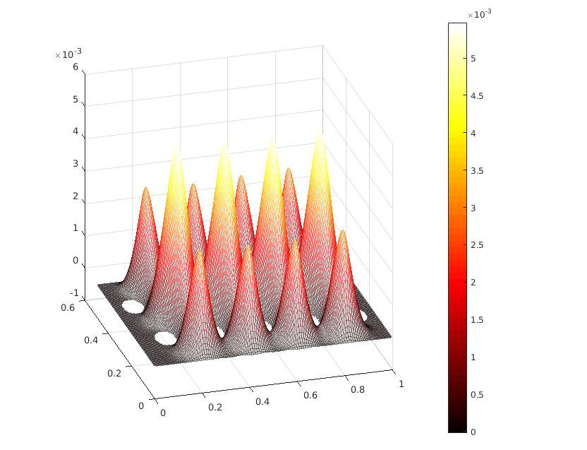 Figure 1
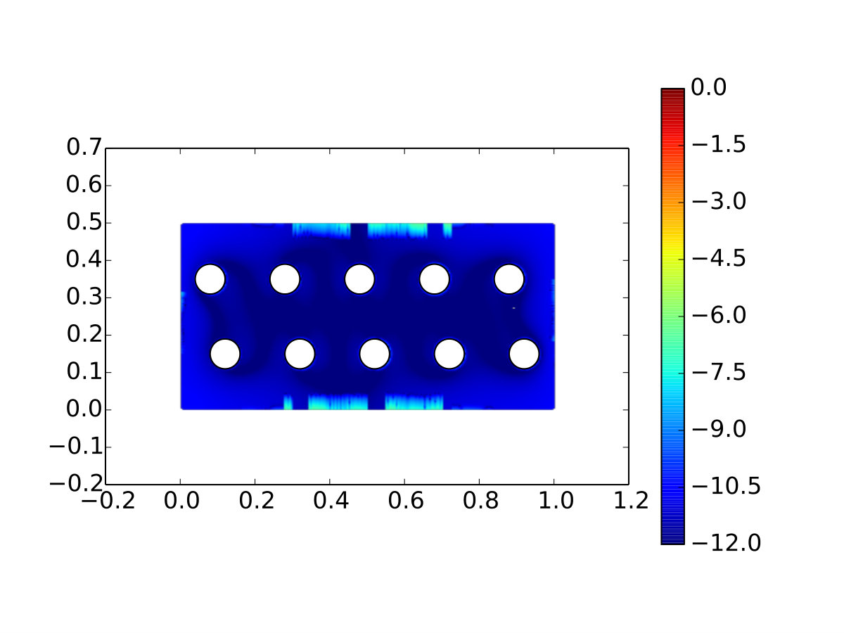 Figure 2
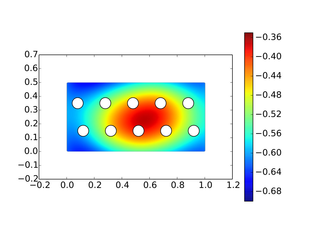 Figure 3
Peer Reviews
No public reviews on file for this paper yet. If you reviewed it on a platform where reviews are public (OpenReview, ICLR, NeurIPS, ICML), you can paste yours below so the community can read it here.
Videos
No videos yet. Explain this paper in a talk, walkthrough, or lecture? Add one.
Integral equation formulation of the biharmonic Dirichlet
problem
M. Rachh
T. Askham
Applied Mathematics Program, Yale University, New Haven, CT 06511
Department of Applied Mathematics, University of Washington, Seattle, WA 98195-3925
Abstract
We present a novel integral representation for the biharmonic Dirichlet problem. To obtain the representation, the Dirichlet problem is first converted into a related Stokes problem for which the Sherman-Lauricella integral representation can be used. Not all potentials for the Dirichlet problem correspond to a potential for Stokes flow, and vice-versa, but we show that the integral representation can be augmented and modified to handle either simply or multiply connected domains. The resulting integral representation has a kernel which behaves better on domains with high curvature than existing representations. Thus, this representation results in more robust computational methods for the solution of the Dirichlet problem of the biharmonic equation and we demonstrate this with several numerical examples.
keywords:
integral equations , biharmonic , Dirichlet , multiply connected
††journal: J. Comput. Phys.
1 Introduction and problem formulation
A variety of problems of mathematics and physics require the computation of a biharmonic potential subject to Dirichlet boundary conditions. The pure bending problem for an isotropic and homogeneous thin clamped plate is a classical application. Another application is the computation of a extension of a given function from its domain of definition to a larger, enclosing domain (we discuss these applications further in section 2.1).
The Dirichlet problem is given as follows. For a domain with boundary , find a function such that
[TABLE]
where and are continuous functions defined on .
The use of standard finite difference methods for the solution of 1, 2 and 3 is complicated greatly by the fact that the differential equation is fourth order. For instance, the resulting linear system for a discretization with nodes in each dimension would have a condition number proportional to , which poses several concerns for obtaining high accuracy solutions for large problems.
Integral equation methods, on the other hand, have many advantages for such problems. Because 1, 2 and 3 is homogeneous, the resulting integral equation is defined on the boundary alone and there is a reduction in the dimension of the problem. Complex geometries are handled more easily by an integral equation and, with appropriate choice of representation, the discrete problem tends to be as well conditioned as the underlying physical problem, independent of the system size [1]. One challenge for integral equation methods is that the resulting linear systems are dense. However, there are many well developed fast algorithms for the solution of these systems, most descending from the fast multipole method (FMM) [2].
Integral representations for the solution of 1, 2 and 3 have been developed previously. In particular, the problem is addressed in Peter Farkas’ thesis [3] and the method presented there has been extended to three dimensions in [4]. The integral kernels derived in [3] are taken to be linear combinations of derivatives of the fundamental solution of the biharmonic problem. Assuming the boundary is a smooth curve, the combinations are chosen to maximize the smoothness of the integral kernel as a function on the boundary (for smooth domains). However, the integral kernels derived for 1, 2 and 3 have a leading order singularity of on a domain with a corner. Because of this singularity, designing quadrature rules for discretizing the integral equation is difficult for domains with corners. Furthermore, the resulting discretized system has large condition numbers for domains whose boundaries have high curvature.
For the related problem of two dimensional steady Stokes flow, the stream function formulation results in a biharmonic equation with the gradient of the biharmonic potential specified on the boundary. Let be the stream function for Stokes flow with no slip boundary conditions, then
[TABLE]
for appropriately chosen functions and . Over the past century, much work has been done to develop integral representations for the biharmonic problem in this setting, as well as the similar setting of the Airy stress function formulation of the plane theory of elasticity [5, 6, 7, 8]. The representations given in the above references typically have more benign singularities than the representation presented in [3]. In particular, the representation used in this paper, taken from [5, 6], has a leading order singularity of on domains with corners. Moreover, this representation (and others from the above references) can be expressed in terms of Goursat functions, allowing for a convenient representation of the stream function. Because of these advantages, we choose to adapt the representation of [5, 6] to solve 1, 2 and 3.
This adaptation is not immediate. First, in two dimensional Stokes flow, the physical quantities of interest are derivatives of the biharmonic potential and not itself; the representation of from [5, 6] is not necessarily single-valued. Second, in converting the boundary conditions 2 and 3 into the boundary conditions 5 and 6, the data is differentiated along the curve so that the original boundary condition is only met up to a constant. These issues are addressed here, with particular attention paid to the case of multiply connected domains. More precisely, we will show that the desired (and uniquely defined) potential can be expressed in terms of (possibly) multi-valued Goursat functions.
The rest of the paper is organized as follows. In section 2, we present some mathematical preliminaries, including the notation used throughout the paper, a review of the Farkas integral representation, and a review of the completed layer potential representation for solving 4, 5 and 6 in terms of the Goursat functions. In section 3, we explain how to adapt the Stokes layer potentials for the Dirichlet problem, present an integral representation for solving 1, 2 and 3, and prove the invertibility of the resulting integral equation. We outline the numerical tools we used to solve this integral equation and present some numerical results in section 4. In section 5, we provide some concluding remarks and ideas for future research.
2 Preliminaries
The notation for the following concepts can be cumbersome and an attempt has been made to stay consistent. Vector-valued quantities are denoted by bold, lower-case letters (e.g. ), while tensor-valued quantities are bold and upper-case (e.g. ). Subscript indices of the non-bold character (e.g. or ) are used to denote the entries within a vector or tensor. We use the standard Einstein summation convention, i.e., there is an implied sum taken over the repeated indices of any term. The vectors and are reserved for spatial variables in , while and are reserved for spatial variables in . We make the standard identification between points in and points in , i.e. the point is equivalent to the point , and we switch between the two notions implicitly in much of what follows. For integration, the symbol is used to denote an integral with respect to arc length and the symbol is used to denote a complex contour integral. Script letters , , and are reserved for Banach spaces. denotes the identity operator on .
Let will denote a bounded, possibly multiply-connected, domain in with a smooth boundary (unless otherwise noted). For a domain with holes, we will denote the outer boundary by and the boundary of each hole by , so that . Let denote the outward unit normal and the positively-oriented unit tangent for . If we need to distinguish between the exterior and interior of , we will let denote the interior and denote the exterior.
2.1 Applications of the biharmonic Dirichlet problem
Consider the pure bending of an isotropic and homogeneous thin clamped plate. In the Kirchoff-Love theory, the vertical displacement of the plate, , satisfies the equations
[TABLE]
where represents the midline of the thin plate, is its boundary, and is the transverse load applied to the plate. Using standard techniques, the above problem can be reduced to a homogeneous biharmonic problem of the form 1, 2 and 3.
In a recent paper, [9], it was shown that the solution of polyharmonic Dirichlet problems can be used as part of the solution of inhomogeneous PDEs on complex geometries. We will breifly review this procedure here.
Consider the Poisson equation
[TABLE]
A particular solution, , which satisfies 10 can be obtained from the formula
[TABLE]
where is some domain such that and is a function defined on which satisfies .
There are rapid methods for evaluating the integral 12 in the case that is a box. However, it is unclear how best to define (and compute) the values of on , particularly such that is smooth across the boundary of . One approach is to compute the extension as the solution of a homogeneous PDE on the exterior.
Suppose that solves
[TABLE]
which is a problem of the form 1, 2 and 3. Then, setting and makes a function across .
In [9], a extension was computed as the solution of a Laplace problem on . This was found to accelerate the convergence of the Poisson solver over discontinuous extension (i.e. to be zero outside of ). By computing a smoother extension, as in the solution of the problem above, the efficiency and robustness of the Poisson solver could be further improved. For a PDE-based version of this approach, see [10].
2.2 The Farkas integral representation
As mentioned in the introduction, there are existing integral representations for the solution of 1, 2 and 3. In [3], the solution is given as the sum of two layer potentials, i.e.
[TABLE]
where and are unknown densities.
The integral kernels, and are based on derivatives of the Green’s function for the biharmonic equation. For two points on the plane, and , the Green’s function is given by
[TABLE]
Let and . Then,
[TABLE]
More explicitly, we have
[TABLE]
On enforcing the Dirichlet boundary conditions for , we obtain the integral equation
[TABLE]
where denotes the signed curvature as a function on and is a point on . The kernels are given by , ,
[TABLE]
For a sufficiently smooth and simply connected domain, the integral equation 20 is invertible. The case of a multiply connected domain is not treated fully in [3], but some of the issues are considered.
As mentioned above, the kernels and are constructed with the goal that the are as smooth as possible. Suppose that the boundary is of class . Then, the kernels, , are functions on the boundary for each [3]. Therefore, on a smooth boundary, these kernels are smooth. However, on a domain with a corner, it is clear from the formula 21 that the kernel has a singularity with strength . This singularity, in addition to the term in 20 which explicitly involves the curvature, makes the representation 14 unstable for domains with high curvature (or corners).
2.3 Stokes flow in the plane
The equations of incompressible Stokes flow with no-slip boundary conditions on a domain with boundary are
[TABLE]
where is the velocity of the fluid and is the pressure. Following standard practice, the velocity can be represented by a stream function . Let
[TABLE]
so that the divergence-free condition, 24, is satisfied automatically. Taking the dot product of with 23 results in a biharmonic equation for . In particular, is a biharmonic function which satisfies 4, 5 and 6 with and .
2.4 Goursat functions
Goursat showed that any biharmonic function can be represented by two analytic functions and (called Goursat functions) as
[TABLE]
where and [11]. In solving equation 4, 5 and 6, we are interested in and . Muskhelishvili’s formula [12] gives an expression for these quantites in terms of the Goursat functions as
[TABLE]
We say that a pair of Goursat functions and is equivalent to a Stokes velocity field if the biharmonic function defined by 27 is such that .
The references [5, 6, 7, 8] give many options for the representation of and as layer potentials of a complex density given on the boundary of the domain. Of computational interest, representations for and exist such that enforcing the boundary conditions of 4, 5 and 6 results in an invertible second-kind integral equation (SKIE) for the density.
2.5 Integral representations for Stokes flow in the plane
We will first present the single layer and double layer potentials of Stokes flow in the Stokeslet/stresslet formulation, which may be more familiar. For details concerning these ideas, see, inter alia, [13]. We will then present their equivalent potentials in the classical Goursat function formulation. The reason for doing so is two-fold: first, the Goursat formulation makes it more natural to evaluate the stream function ; second, the complex variables-based Goursat formulation is readily adaptable for efficient fast multipole methods.
2.5.1 Stokes layer potentials
The Green’s function for the incompressible Stokes equations in free space, or Stokeslet, is given by
[TABLE]
The vector field represents a Stokes velocity field at due to a point force applied at . For a continuous distribution of surface forces on a curve , the induced Stokes field, called a single layer potential, is given by
[TABLE]
The following lemma describes the behavior of the Stokes single layer potential as a function on , see [13] for details.
Lemma 1**.**
Let denote a single layer Stokes potential of the form 30. Then, satisfies the Stokes equations in and is continuous in .
The Stokes single layer potential has equivalent Goursat functions, and , which can be expressed in terms of complex layer potentials:
[TABLE]
where , , and . The stream function corresponding to this Goursat function pair is then
[TABLE]
Note that, the velocity field associated with the stream function is given by
[TABLE]
Another quantity of physical interest in Stokes flow is the stress tensor ; for a Stokes velocity field and pressure , it is given by
[TABLE]
The stress tensor , or stresslet, associated with the Green’s function is given by
[TABLE]
The vector field represents the velocity field resulting from a stresslet with strength oriented in the direction at . For a distribution of stresslets on a curve , the induced Stokes field, called a double layer potential, is given by
[TABLE]
The following lemma describes the behavior of the Stokes double layer potential as a function on , see [13] for details.
Lemma 2**.**
Let be a curve, denote the exterior of the curve, denote the interior, denote a double layer Stokes potential of the form 38, and . Then, satisfies the Stokes equations in and the jump relations:
[TABLE]
In the above, denotes a Cauchy principal value integral and denotes the double layer potential with the integral taken in the principal value sense.
The double layer potential above has equivalent Goursat functions, and , which can be expressed in terms of complex layer potentials:
[TABLE]
where , and are as above. The stream function corresponding to this Goursat function pair is then
[TABLE]
As before, the velocity field associated with the stream function is given by
[TABLE]
2.5.2 The completed double layer representation for Stokes
flow
Using the layer potentials described above, we can represent the solution of , or equivalently the system 23, 24, and 25, in terms of a density given on the boundary of the domain. The completed double layer representation [6] for the velocity is
[TABLE]
where , and the representation of an equivalent pair of Goursat functions, giving a stream function , can be inferred from the formulas of the previous subsection. When the no-slip boundary conditions are enforced for this representation, the result is an invertible SKIE for the density . The reader can refer to [6] for a detailed discussion of the Fredholm alternative for this representation. We summarize it as
Lemma 3**.**
Let be defined as in 46 and . Then
[TABLE]
For a sufficiently smooth curve , the operator is a compact operator on , where is or for . Further, the integral equation
[TABLE]
is invertible, even for multiply connected domains.
For the above integral equation, the singularities of the integral kernels which define are at worst order , even for a boundary with a corner.
3 Integral equation derivation
We would like to adapt the completed double layer representation for solutions of Stokes flow 4, 5 and 6 to solve the clamped plate problem 1, 2 and 3. Let and be the boundary data as in 1, 2 and 3. By computing tangential derivatives of on each boundary component, we get the following related Stokes problem:
[TABLE]
There are two main issues to be addressed in using the completed double layer representation in this context. First, the representation is designed for Stokes flow, in which the quantities of interest are derivatives of the potential and not itself; the representation for may not be single-valued. We will establish that, in the context of 49, the stream function is necessarily single-valued. We also discuss some numerical issues related to evaluating the stream function. The second issue to address is that the solution only satisfies the original boundary condition for the value of up to a constant on each boundary component. In fact, for multiply connected domains, the completed double layer representation is incomplete for the Dirichlet problem 1, 2 and 3. We present a remedy for this issue and provide some physical intuition.
3.1 Single-valued stream functions
To solve the Dirichlet problem 1, 2 and 3, it is necessary to compute a single-valued biharmonic potential. In the case of a multiply connected domain, there is no guarantee that a single-valued stream function exists for a given velocity field.
Consider the following example. Let denote standard polar coordinates. It is easy to verify that the velocity field solves the equations of Stokes flow in an annulus centered at the origin. A stream function for this flow is , which is not single-valued; indeed, there are no single-valued stream functions which generate this flow.
Let be a multiply connected domain with boundary , as in the previous section. We note that the gradient of a stream function is determined by the velocity field, i.e.
[TABLE]
Therefore, a velocity field has single-valued stream functions if and only if is conservative. Using standard results from multivariable calculus, we can characterize such flows.
Proposition 1**.**
Suppose that is a divergence-free velocity field which is on and continuous on . The field is conservative if and only if
[TABLE]
The equalities 51 constitute linearly independent constraints on the boundary data because the divergence-free condition 24 implies that . It turns out that these conditions are satisfied when the Dirichlet problem is recast as a Stokes flow 49, as it is easily verified that
[TABLE]
Thus, any stream function obtained for the Stokes flow 49 is necessarily single-valued.
3.2 Evaluating the stream function
Given compatible boundary data for the velocity field , the completed double layer representation for Stokes flow 46 guarantees the existence of a solution density and a corresponding stream function . The Goursat function formula for , see section 2.5.1, is necessarily single-valued, as explained above, but it is not immediately obvious from the formula that this should be true.
The difficulty in the representation of comes from the part of the stream function corresponding to the double layer potential 44. The second term in the expression for the double layer potential is
[TABLE]
To compute this term, in a naïve numerical implementation, the question of which is the appropriate branch of the logarithm to use would arise at many steps. To avoid this complication, it is possible instead to compute , up to a constant, as the harmonic conjugate of the function
[TABLE]
We will use this approach to evalute numerically. As a result of the Cauchy-Riemann equations, the harmonic conjugate of , satisfies the following Neumann problem for the Laplace equation:
[TABLE]
It is possible then to use standard integral equation methods to compute .
Let , where is the single layer potential for Laplace’s equation, given by
[TABLE]
where , for some , is an unknown density (see [1, 14]). Imposing the Neumann boundary conditions results in the following boundary integral equation for :
[TABLE]
where the operator is compact, so that the integral equation is second kind. For a derivation of this result, see [1].
It is well known that the operator has a one dimensional null space. Thus, we choose to solve the above integral equation subject to the constraint . Furthermore, it is known that solving the Neumann problem subject to the above constraint is equivalent to solving
[TABLE]
where .
3.3 Making the representation complete
As mentioned above, the solution of the auxiliary Stokes problem 49 only satisfies the boundary conditions of the original Dirichlet problem 1, 2 and 3 up to a constant on each boundary component. For a simply connected domain, this constant can be recovered from the fact that adding an arbitrary constant to a stream function does not change the velocity field. Thus, in simply connected domains, there is an equivalence in the solutions of 49 and 1, 2 and 3.
To analyze the case of a multiply connected domain, we first consider radially symmetric solutions on an annulus centered at the origin. Let be a radially symmetric biharmonic potential. Then solves the ordinary differential equation (ODE)
[TABLE]
Four linearly independent solutions of this ODE are , , , and . For each solution, we can compute the associated velocity field . By construction, satisfies the continuity condition 24. For the momentum equation 23 to be satisfied, we need that is a conservative vector field, which is equivalent to the condition that for any closed loop in the annulus. For the first three linearly independent solutions, so that is trivially a conservative vector field. The fourth solution, on the other hand, has . By considering a curve encircling the origin, we see that is not a conservative vector field and that any pressure for the velocity field associated with is not single-valued.
The function is the Green’s function for the biharmonic equation and is the equivalent of a charge for such problems. The above analysis can be extended to show that any solution of the biharmonic equation with net charge cannot be represented as a Stokes velocity field. In simply connected domains, since , there can be no net biharmonic charge in the domain. For multiply connected domains with genus , the set of stream functions for Stokes velocity fields misses an dimensional space of solutions, corresponding to biharmonic charges located in the holes of the domain. Following this reasoning, we obtain a complete representation for biharmonic potentials on multiply connected domains by adding charges, one per each hole of the domain, to the representation for . The details of this approach, and the proof that it is sufficient, is in the next section.
3.4 The integral representation
Following the discussion in the previous two sections, it is now possible to present an integral representation for the Dirichlet problem of the biharmonic equation based on the completed double layer representation for the Stokes problem. We first fix some notation. Let be a multiply connected domain, with boundary , as in the previous sections. For each boundary component , let be its interior and be a point in . Then, let the solution be represented in terms of layer potentials and biharmonic charges as
[TABLE]
where is an unknown density, the are unknown constants, the distance from to is , and the operators and map complex densities to the stream functions corresponding to single and double layer potentials, as defined in section 2.
Remark 1**.**
As discussed in section 3.2, we will only evaluate the operator up to a constant in our numerical implementation. However, this does not affect the analysis of this section because of the freedom in choosing .
As before, we can identify a real, vector-valued density with by setting . Let be the velocity field corresponding to the stream function . Then, in terms of , we have
[TABLE]
where and are the single and double layer potentials for the density , as defined in section 2.
Let and . Assume that the boundary data for the Dirichlet problem 1, 2 and 3 satisfies and , a slightly stronger assumption on the regularity of than given in the original problem statement. Denote the integrals of around each boundary component by . To solve equation 1, 2 and 3, we impose the boundary conditions on the gradient of as in 49 on the above representation for , or, equivalently, the no-slip boundary conditions 25 on the above representation for with
[TABLE]
Under the assumptions on and , the boundary data .
Let denote the part of the velocity field due to the charges, i.e.
[TABLE]
Then, due to lemmas 1 and 2, enforcing the boundary condition for each results in the following boundary integral equation
[TABLE]
To ensure that the values of are correct on the boundary, further constraints are needed. We impose additional conditions on the value of
[TABLE]
where the constants are as defined above. The integral of about each component can be written in terms of the unknowns as
[TABLE]
Combining equations 67, 68, and 70, we get the following linear system for the unknowns and
[TABLE]
where , , and .
Proposition 2**.**
The block system 71 is an invertible Fredholm operator.
Proof.
It is simple to show that the linear system 71 is Fredholm. The block which contains is Fredholm due to lemma 3. The off-diagonal blocks, denoted by and , are trivially compact because either the domain or range of the operator is finite dimensional. Finally, is Fredholm because it is a finite-dimensional linear operator. Therefore, the full system is Fredholm.
Due to the Fredholm alternative, it is only necessary to establish the injectivity of the system 71 to prove that it is invertible. It is clear that if and solve equation 71, then the resulting solution, , given by 62, solves the original Dirichlet problem 1, 2 and 3. By construction, is biharmonic in . Moreover, satisfies and on the whole boundary and for each boundary component , so that the boundary conditions are satisfied.
In the case that and , we have that for the Dirichlet problem. By the uniqueness of solutions to 1, 2 and 3, this implies that in . It is, however, less immediate that implies that and .
For each , let be a curve which satisfies , where represents the winding number of the curve about z. Because and in , we have
[TABLE]
Let . We observe that corresponds to a Stokes velocity field in for any . Let be its associated pressure. Then
[TABLE]
Further, a simple calculation shows that
[TABLE]
for . Combining these equations, we conclude that
[TABLE]
Thus for .
The first row of the system 71 then reads
[TABLE]
From the invertibility of , we conclude that . Because and for , we get that . It then follows that as well, proving the injectivity of the system. ∎
4 Results
We first review the existing numerical tools used to compute solutions of the integral equation 71. To discretize the integral equations, we use the Nyström method. We divide the boundary into panels and represent the unknown density and the boundary data by their values at scaled Gauss-Legendre nodes on each panel. Let denote the number of Gauss-Legendre panels. We discretize each panel using 16 scaled Gauss-Legendre nodes. Then is the number of discretization points on the boundary. Let denote the discretization nodes, denote the appropriately scaled Gauss-Legendre quadrature weights for smooth functions, and denote the unknown density at . When forming the linear system, we use scaled unknowns, , so that the spectral properties of the discrete system with respect to the norm are approximations of the spectral properties of the continuous system as on operator on (for more on this point of view, see [15]). The integral kernels in this paper are either smooth or have a weak (logarithmic) singularity. For the smooth kernels in the integral representation, we use standard Gauss-Legendre weights appropriately scaled. For kernels with a logarithmic singularity, we use order generalized Gaussian quadrature rules [16, 17].
After applying the integral rule, we obtain a linear system for the unknowns. This system is typically well-conditioned, but dense. Let denote the discretized linear system of size corresponding to the integral equation (71). Let denote the condition number of the discretized matrix . For our applications, the system size was modest and we computed the unknowns and using Gaussian elimination. For larger applications, the system is amenable to solution by any of a variety of iterative or fast-direct solvers, which we will not review here.
For the visualizations in this section, we evaluate the layer potentials inside the domain, with some points being very close to the boundary. The value of the layer potential can be difficult to evaluate at such points because of the near-singularity in the integral kernel. We use a sixth order quadrature by expansion method [18, 19] to evaluate these integrals efficiently and accurately.
In this section we consider two test cases. The first example is a convergence study for a simply connected domain to demonstrate the order of convergence for the discretized integral equation. We also compare the condition numbers for the discretized linear systems corresponding to our integral representation and the existing integral representation by Farkas [3] for a family of simply connected domains with increasing curvature. For the second example, we demonstrate the order of convergence and compute the Green’s function for a multiply connected domain. For all examples except the computation of the Green’s function, the boundary data and are chosen corresponding to a known solution of the biharmonic equation in given by
[TABLE]
where are uniformly chosen from . Let denote the computed solution at targets in the interior of , and let denote an estimate for the error given by
[TABLE]
4.1 Simply connected domain examples
Let denote the interior of a rounded rectangular bar with length , height , and vertices at . Following the procedure discussed in [20], the corners are rounded using the Gaussian kernel
[TABLE]
with . The boundary data and are chosen corresponding to a known solution , defined as in 77, with four sources located at
[TABLE]
with chosen uniformly from .
The potential is evaluated at targets in the interior of ,
[TABLE]
with again chosen uniformly from . A sample geometry with sources and targets and the error as a function of are shown in fig. 1. The convergence study shows that the error decays like a th order convergent scheme.
The integral equation presented in this paper is significantly better conditioned than the existing integral equation discussed in [3] — particularly when the boundary has regions with large curvature. We plot the condition number of the discretized system of integral equations for the representations given by both 71 and 20 as a function of the rounding parameter for the rounded rectangular bar in fig. 2. The maximum curvature of the boundary is directly proportional to . The condition number increases linearly with the maximum curvature for integral equation 20, but is independent of the curvature for the integral equation presented in this paper.
4.2 Multiply connected domain - examples
Let now denote the interior of a multiply connected domain, where the outer boundary is the boundary of the rounded rectangular bar discussed above with rounding parameter and the domain has ten circular obstacles with radii and centers located at ,
[TABLE]
We will first perform a convergence study, as above, with a known solution defined in terms of point sources according to 77. We create ten sources, one located inside each obstacle, whose locations are given by
[TABLE]
where are chosen uniformly from . The potential is then tested at twelve targets located at
[TABLE]
where are chosen uniformly from .
We observe th order convergence in the error even for this example. The error as a function of the number of discretization points along with a sample geometry are shown in fig. 3. We also plot the field, and the error in evaluating the potential in the volume using a sixth order quadrature by expansion method in fig. 4. We note that the error observed near the boundary is larger than at the targets used for the convergence study; this is a result of the relatively low order of the quadrature by expansion method and could be improved by increasing the number of points on the boundary.
For the final example, we compute the function which satisfies the PDE
[TABLE]
where is the two dimensional radially symmetric Dirac delta function centered at and are defined in 78. This function describes the vertical displacement of an isotropic and homogeneous thin clamped plate with a transverse load given by point forces at the points . It is also, by definition, a linear combination of the domain Green’s function , as in
[TABLE]
To compute , we first obtain a particular solution which satisfies the PDE in the volume and add to it the solution of a homogeneous problem to fix the boundary conditions. We have
[TABLE]
where
[TABLE]
and satisfies the following homogeneous biharmonic equation,
[TABLE]
We plot the computed solution in fig. 5.
5 Conclusion
We have presented an integral representation for the biharmonic Dirichlet problem which is stable for domains which have a boundary with high curvature and is applicable to domains which are multiply connected. The representation is based on converting the Dirichlet problem into a problem with velocity boundary conditions, so that classical representations for the velocity boundary value problem can be used. While the technique of [3] — in which integral kernels are chosen by optimizing over the derivatives of an appropriate Green’s function — is general and powerful, the spectral properties of the resulting operator are undesirable for boundaries with high curvature or a corner. Indeed, it seems intuitive that all direct representations for the biharmonic Dirichlet problem should suffer in some way: such an approach asks that one of the integral kernels be singular enough to result in a second kind Fredholm equation for the value of the layer potential and smooth enough to result in a first kind Fredholm equation for the normal derivative of the layer potential.
While some of the above is specific to the biharmonic equation, in particular the use of Goursat functions, it is reasonable to expect the approach to generalize to other high order elliptic problems as well. In particular, there are representations for the modified Stokes equations which are analogues of the completed double layer representation used here [13]. The extension of this method to three dimensions is a topic of ongoing research and will be reported at a later date.
Acknowledgments
M. Rachh’s work was supported by the U.S. Department of Energy under contract DEFG0288ER25053, the Office of the Assistant Secretary of Defense for Research and Engineering and AFOSR under NSSEFF Program Award FA9550-10-1-0180, and the Office of Naval Research under award N00014-14-1-0797/16-1-2123. T. Askham’s work was supported by the U.S. Department of Energy under contract DEFG0288ER25053, the Office of the Assistant Secretary of Defense for Research and Engineering and AFOSR under NSSEFF Program Award FA9550-10-1-0180, and the Office of the Assistant Secretary of Defense for Research and Engineering and AFOSR under award FA95550-15-1-0385. The authors would like to thank Leslie Greengard for suggesting this problem and both Leslie Greengard and Shidong Jiang for many useful discussions.
The reference list from the paper itself. Each links out to its DOI / PubMed record.
- 1[1] R. Kress, Linear Integral Equations, Applied Mathematical Sciences, Springer New York, 1999.
- 2[2] L. Greengard, V. Rokhlin, A fast algorithm for particle simulations, Journal of computational physics 73 (2) (1987) 325–348.
- 3[3] P. Farkas, Mathematical foundations for fast methods for the biharmonic equation, Pro Quest LLC, Ann Arbor, MI, 1989, thesis (Ph.D.)–The University of Chicago.
- 4[4] S. Jiang, B. Ren, P. Tsuji, L. Ying, Second kind integral equations for the first kind Dirichlet problem of the biharmonic equation in three dimensions, J. Comput. Phys. 230 (19) (2011) 7488–7501. doi:10.1016/j.jcp.2011.06.015 . · doi ↗
- 5[5] L. Greengard, M. C. Kropinski, A. Mayo, Integral equation methods for stokes flow and isotropic elasticity in the plane, Journal of Computational Physics 125 (2) (1996) 403–414.
- 6[6] H. Power, The completed double layer boundary integral equation method for two-dimensional stokes flow, IMA Journal of Applied Mathematics 51 (2) (1993) 123–145.
- 7[7] H. Power, G. Miranda, Second kind integral equation formulation of stokes’ flows past a particle of arbitrary shape, SIAM Journal on Applied Mathematics 47 (4) (1987) 689–698.
- 8[8] S. G. Michlin, A. H. Armstrong, Integral equations and their applications to certain problems in mechanics, mathematical physics and technology, London, 1957.