Multiple scales and phases in discrete chains with application to folded proteins
Anna Sinelnikova, Antti J. Niemi, Johan Nilsson, Maksim Ulybyshev

TL;DR
This paper introduces a new method to identify and analyze multiple length scales and phase behaviors in chiral heteropolymers like proteins, enhancing understanding of their structure and dynamics.
Contribution
It proposes a systematic approach using a novel order parameter and a variant of Kadanoff's block-spin transformation to distinguish scales and phases in proteins.
Findings
The order parameter reveals multiple length scales in protein structures.
Different phases can coexist at various scales within the same heteropolymer.
The method correlates scales and phases with folding pathway complexity.
Abstract
Chiral heteropolymers such as larger globular proteins can simultaneously support multiple length scales. The interplay between different scales brings about conformational diversity, and governs the structure of the energy landscape. Multiple scales produces also complex dynamics, which in the case of proteins sustains live matter. However, thus far no clear understanding exist, how to distinguish the various scales that determine the structure and dynamics of a complex protein. Here we propose a systematic method to identify the scales in chiral heteropolymers such as a protein. For this we introduce a novel order parameter, that not only reveals the scales but also probes the phase structure. In particular, we argue that a chiral heteropolymer can simultaneously display traits of several different phases, contingent on the length scale at which it is scrutinized. Our approach builds…
Click any figure to enlarge with its caption.
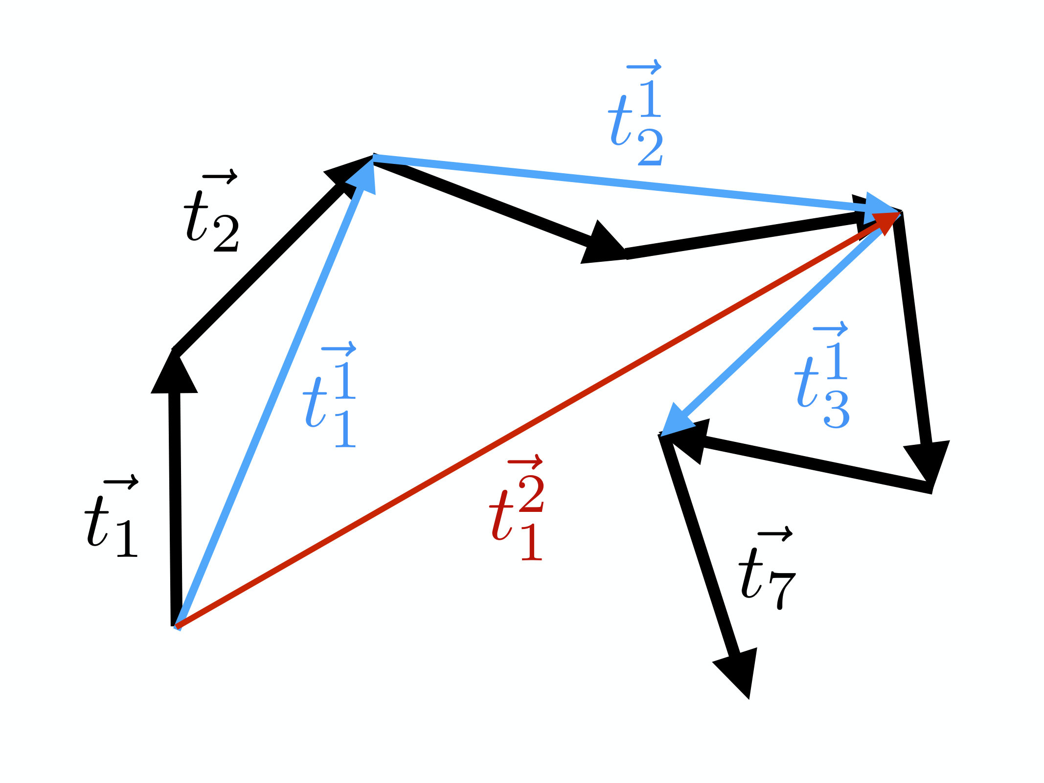 Figure 1
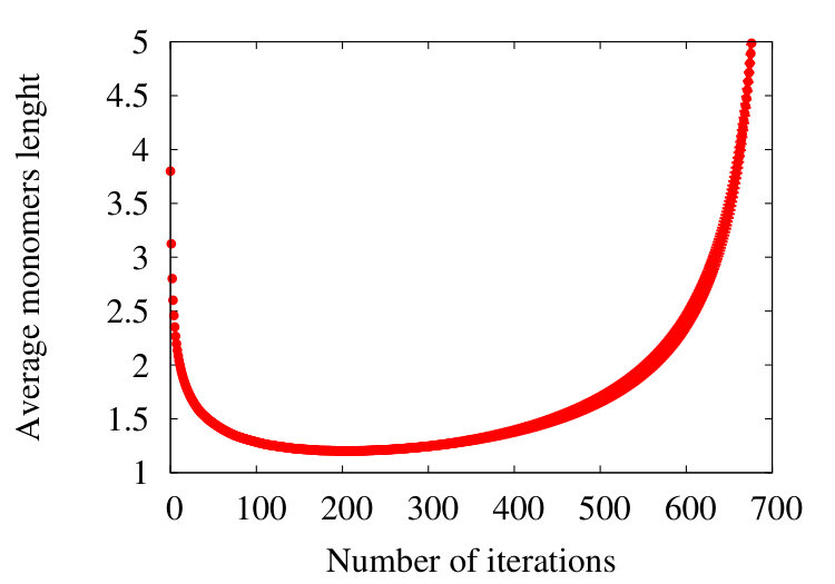 Figure 10
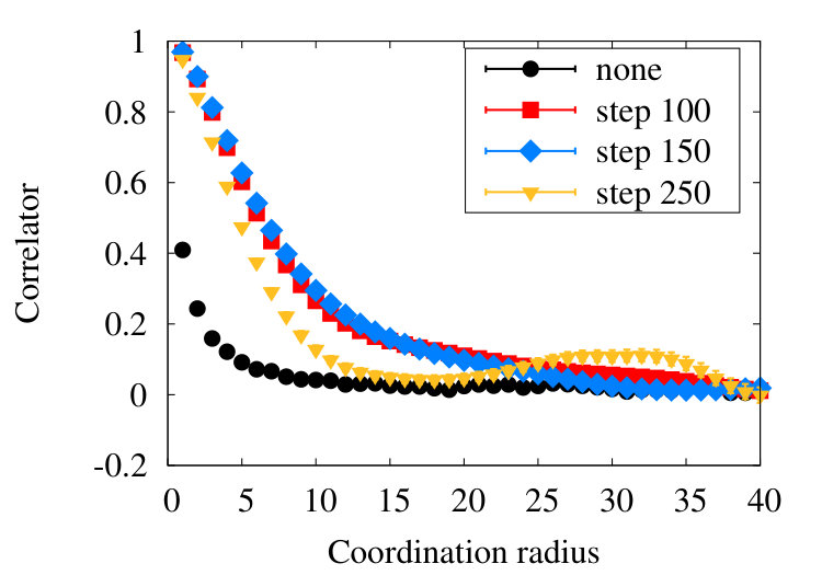 Figure 11
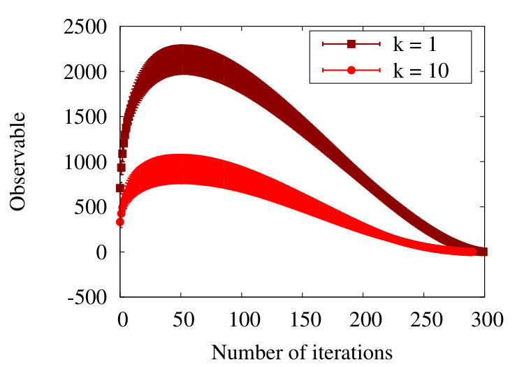 Figure 12
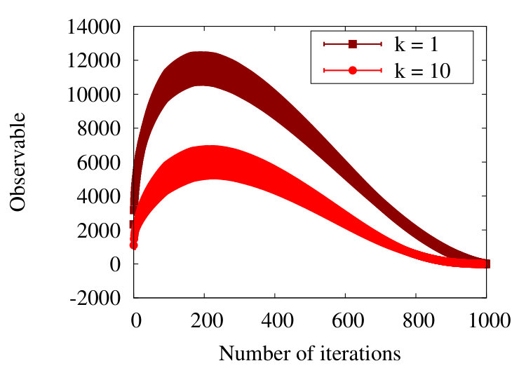 Figure 12
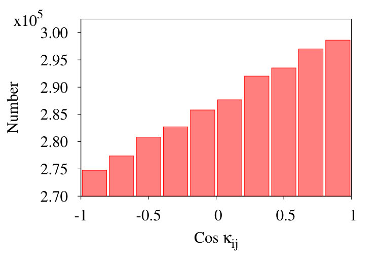 Figure 13
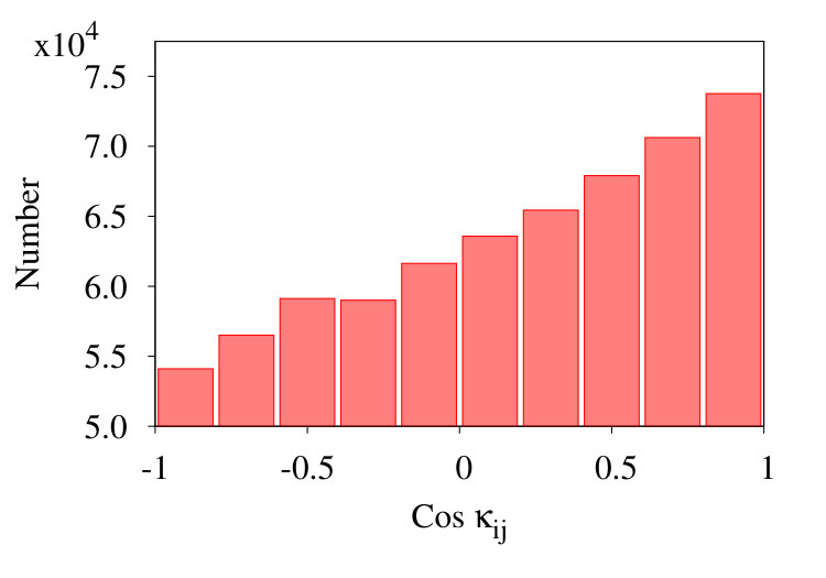 Figure 13
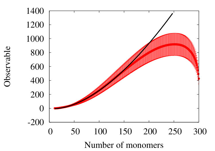 Figure 14
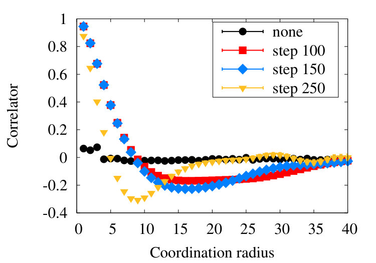 Figure 15
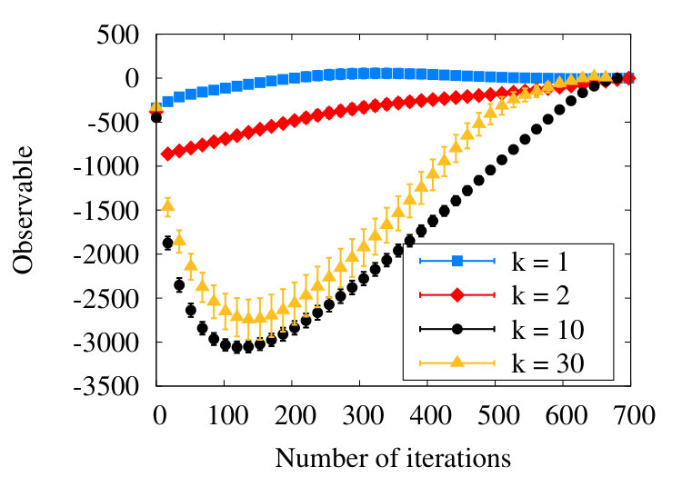 Figure 16
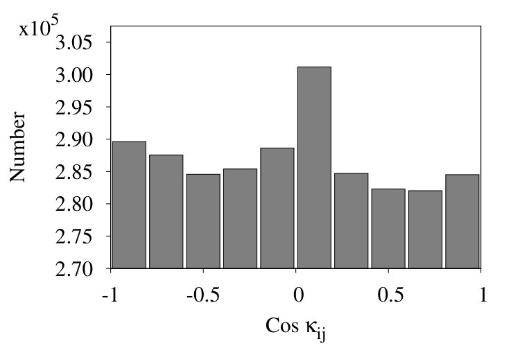 Figure 17
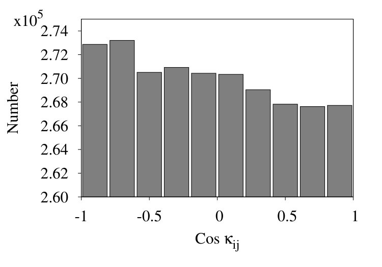 Figure 17
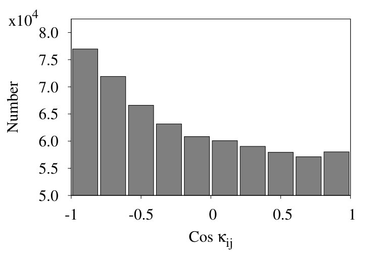 Figure 17
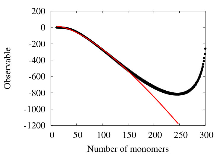 Figure 18
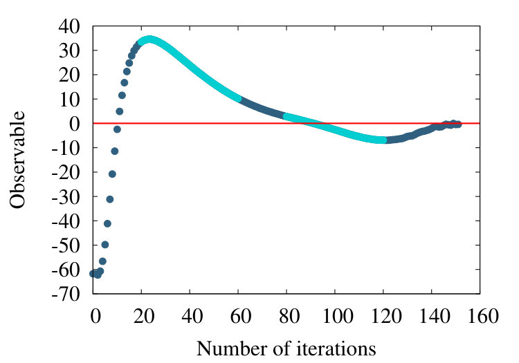 Figure 19
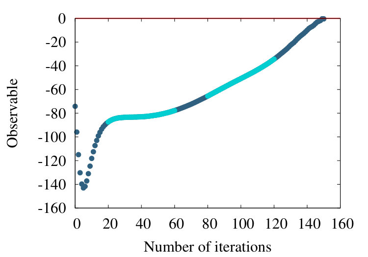 Figure 19
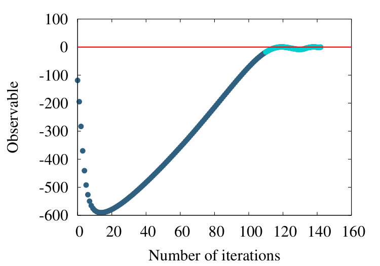 Figure 19
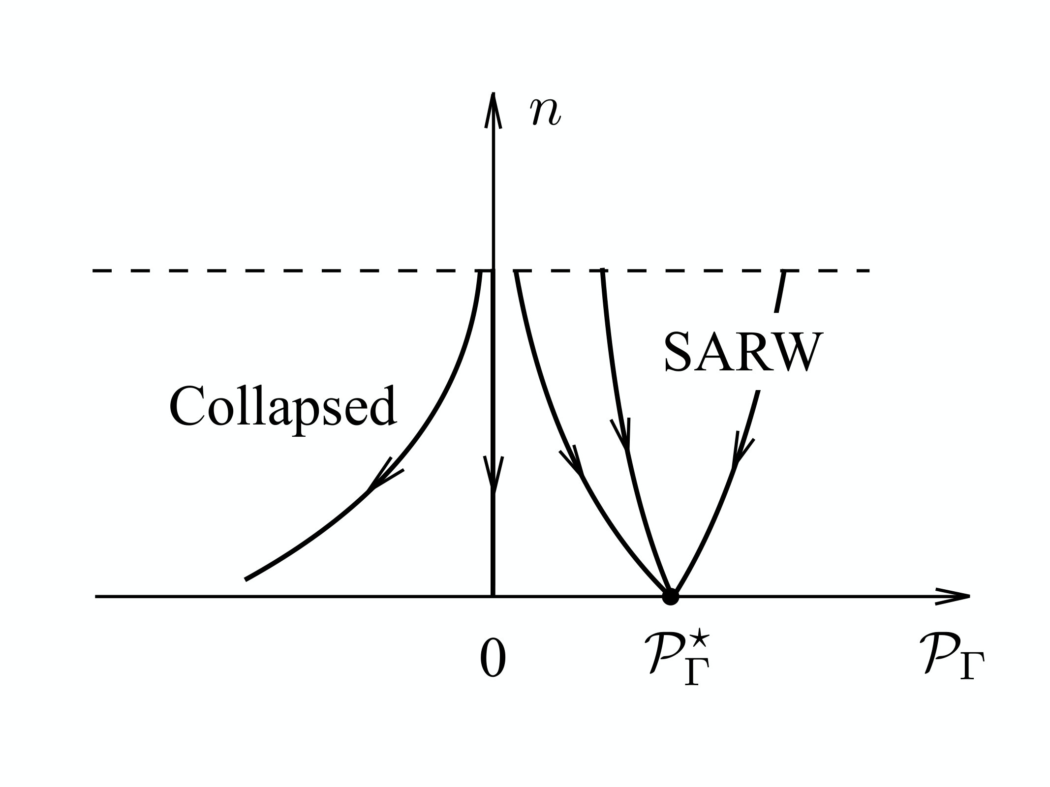 Figure 2
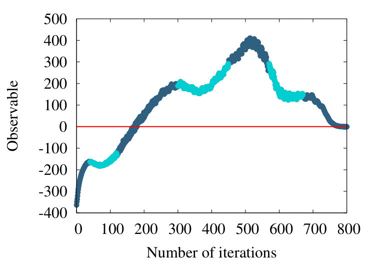 Figure 20
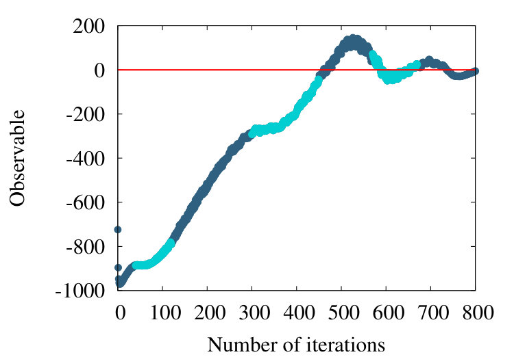 Figure 20
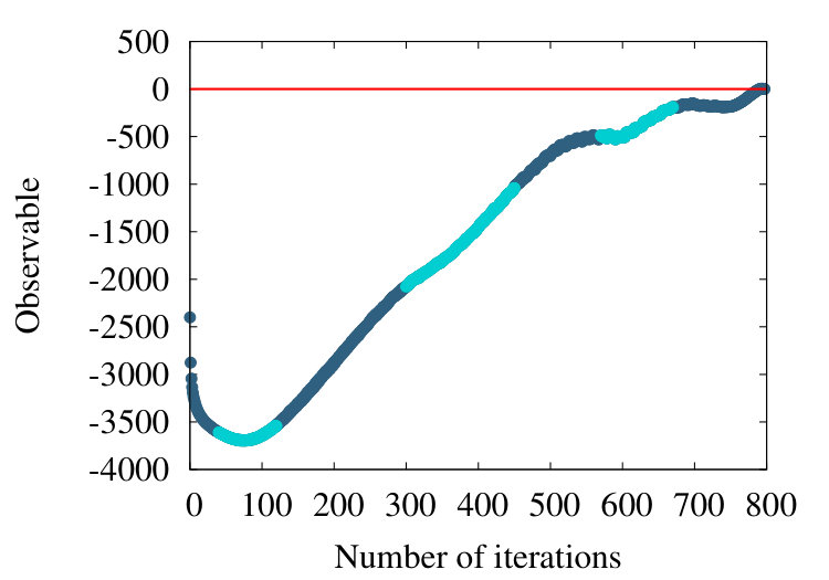 Figure 20
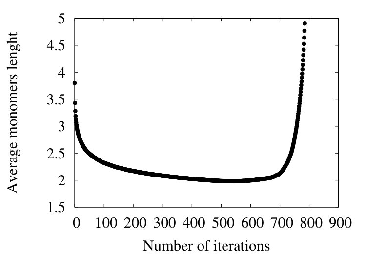 Figure 20
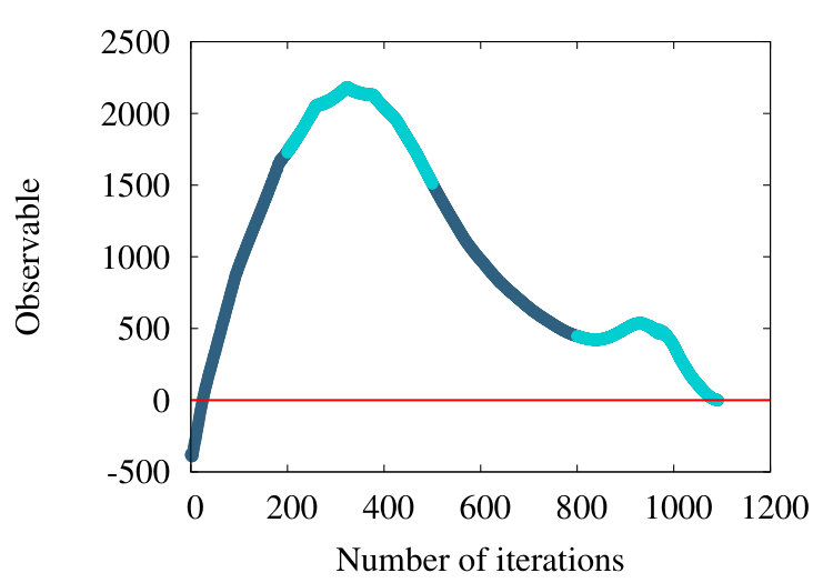 Figure 21
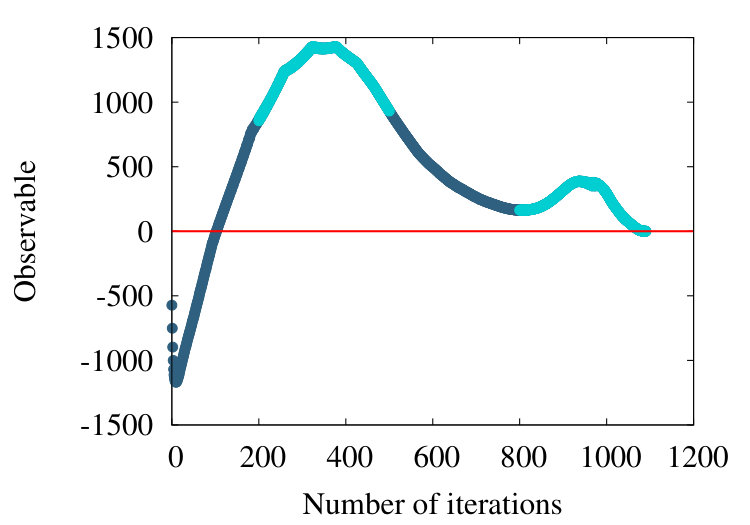 Figure 21
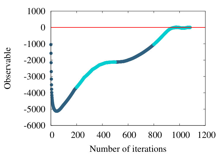 Figure 21
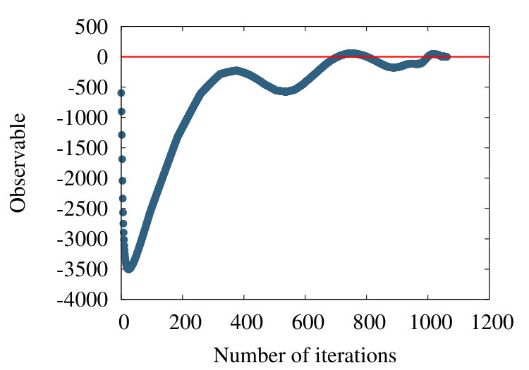 Figure 22
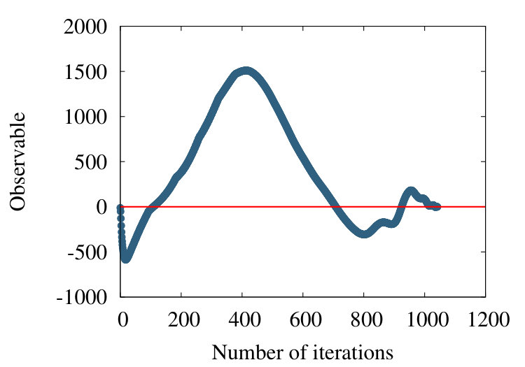 Figure 22
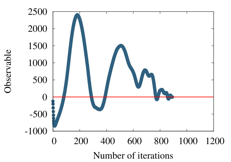 Figure 22
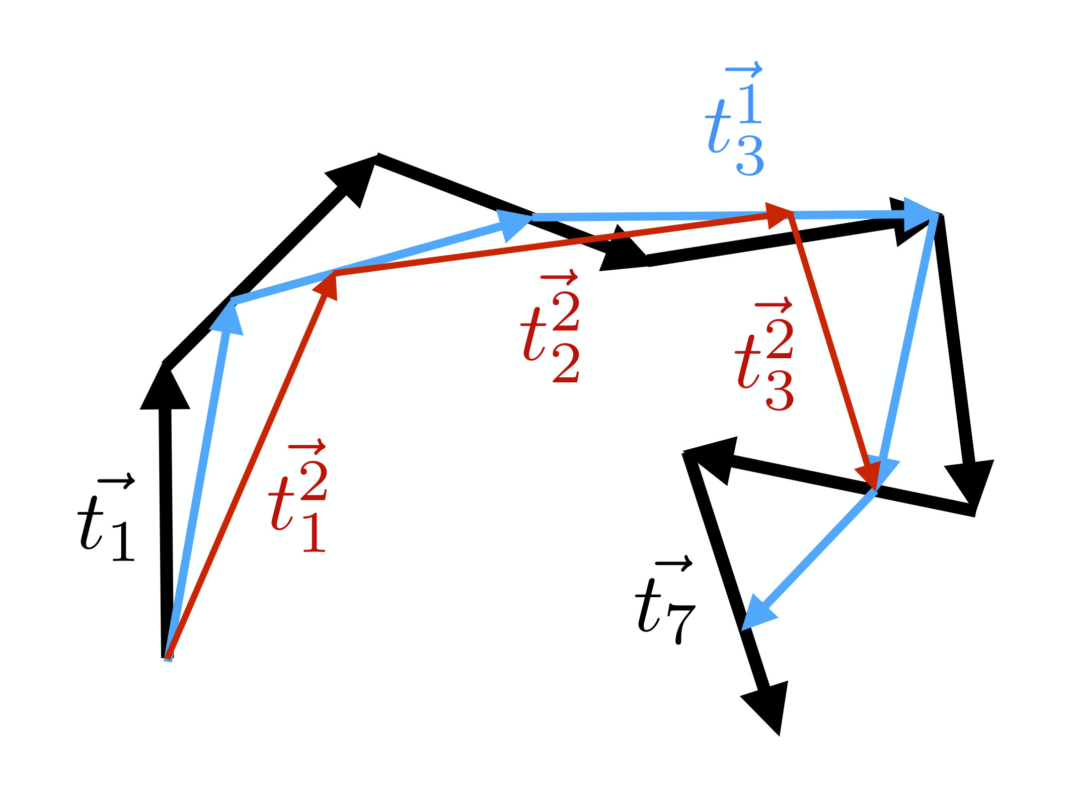 Figure 3
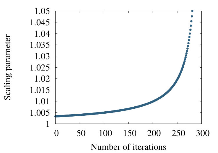 Figure 4
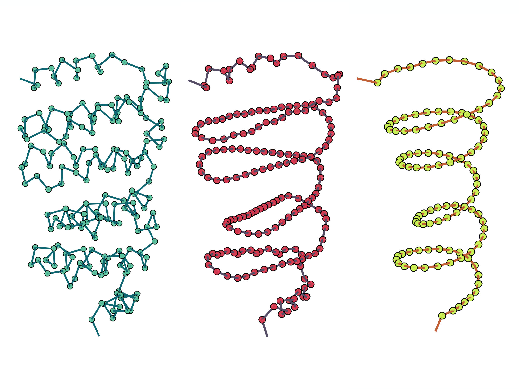 Figure 5
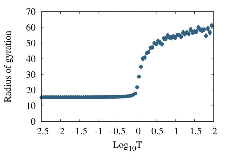 Figure 6
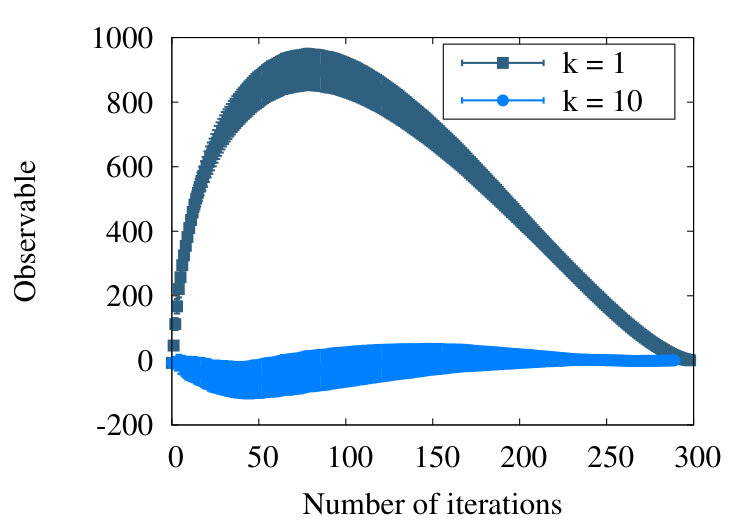 Figure 7
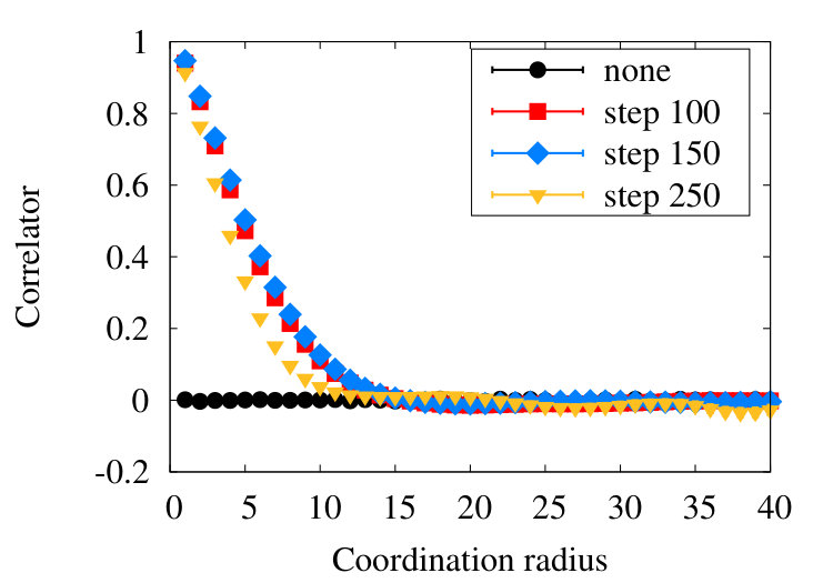 Figure 8
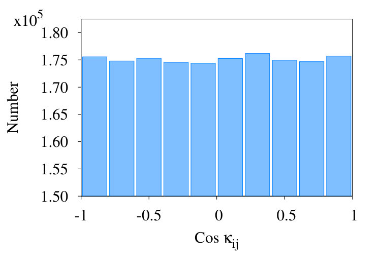 Figure 8
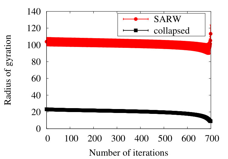 Figure 9
| phase | ||
| Rod | 2 | |
| SARW | 3/2 | |
| RW | = 0 | |
| Collapsed |
Peer Reviews
No public reviews on file for this paper yet. If you reviewed it on a platform where reviews are public (OpenReview, ICLR, NeurIPS, ICML), you can paste yours below so the community can read it here.
Videos
No videos yet. Explain this paper in a talk, walkthrough, or lecture? Add one.
Multiple scales and phases in discrete chains
with application to folded proteins
A. Sinelnikova
Department of Physics and Astronomy, Uppsala University, P.O. Box 516, S-75120, Uppsala, Sweden
A. J. Niemi
[email protected] http://www.folding-protein.org Nordita, Stockholm University, Roslagstullsbacken 23, SE-106 91 Stockholm, Sweden
Department of Physics and Astronomy, Uppsala University, P.O. Box 516, S-75120, Uppsala, Sweden
Laboratory of Physics of Living Matter, School of Biomedicine, Far Eastern Federal University, Vladivostok, Russia
Department of Physics, Beijing Institute of Technology, Haidian District, Beijing 100081, P. R. China
Johan Nilsson
Department of Physics and Astronomy, Uppsala University, P.O. Box 516, S-75120, Uppsala, Sweden
M. Ulybyshev
Institute of Theoretical Physics, University of Regensburg, Universitätsstraße 31, Regensburg, D-93053 Germany
Abstract
Chiral heteropolymers such as larger globular proteins can simultaneously support multiple length scales. The interplay between different scales brings about conformational diversity, and governs the structure of the energy landscape. Multiple scales produces also complex dynamics, which in the case of proteins sustains live matter. However, thus far no clear understanding exist, how to distinguish the various scales that determine the structure and dynamics of a complex protein. Here we propose a systematic method to identify the scales in chiral heteropolymers such as a protein. For this we introduce a novel order parameter, that not only reveals the scales but also probes the phase structure. In particular, we argue that a chiral heteropolymer can simultaneously display traits of several different phases, contingent on the length scale at which it is scrutinized. Our approach builds on a variant of Kadanoff’s block-spin transformation that we employ to coarse grain piecewise linear chains such as the C backbone of a protein. We derive analytically and then verify numerically a number of properties that the order parameter can display. We demonstrate how, in the case of crystallographic protein structures in Protein Data Bank, the order parameter reveals the presence of different length scales, and we propose that a relation must exist between the scales, phases, and the complexity of folding pathways.
pacs:
87.14.et, 02.40.-k, 02.90.+p, 05.65.+bk
I Introduction
A linearly conjugated polymer is conventionally viewed as a piecewise linear polygonal chain, it connects a sequence of vertices that coincide with the locations of its skeletal atoms huggins ; flory1 ; flory2 ; flory3 ; degen ; degen1 ; desc ; edw1 ; degen2 ; edw2 . For example, in the case of a protein the vertices coincide with the positions of the C atoms, and the connecting line segments concur with the diagonals of the peptide planes. Conventionally, a phase is then assigned to the polymer by inspecting the fractal geometry of the chain. For this let () denote the vertices of a given discrete chain . When becomes large the radius of gyration
[TABLE]
admits an asymptotic expansion of the form degen2 ; schafer ; naka ; sokal
[TABLE]
The pre-factor is an effective segment (Kuhn) length. In the case of a polymer its value depends on the atomic level details of the chain and the environment, it is not a universal quantity. The scaling exponent coincides with the inverse Hausdorff dimension of . It is a universal quantity degen2 ; edw2 ; grosberg-1994 ; naka ; sokal ; schafer with a numerical value that does not depend on the atomic level details of the chain. It acts as an order parameter that can detect the phase of the chain. The exponents that characterise the finite size corrections are similarly universal sokal .
In the case of a discrete chain with a homogeneous structure, the scaling exponent is commonly presumed to have only four possible values, corresponding to the four different phases of a homopolymer. At the level of classical mean field theory huggins ; flory1 ; flory2 ; degen2 ; edw2 ; grosberg-1994 ; naka ; sokal ; schafer
[TABLE]
The value of is determined using (2), by successively increasing the number of vertices and by observing how the radius of gyration scales when becomes large. This procedure can work in the case of a homopolymer, when the number of vertices can be increased in an unambiguous manner. Unfortunately, it does not work in the case of a heteropolymer such as a protein, where the amino acid assignment is fixed: There is no unambiguous way to extend the length of a protein, to determine the scaling of its radius of gyration when grows, the number of vertices can not be systematically increased as required by (2). Instead one can try and deduce the value of statistically, by comparing the radius of gyration of a given protein to a statistical pool of different lengths but similar kind of protein structures such as those classified as -helical or -stranded in Protein Data Bank (PDB) pdb . This procedure has some merits, but it lacks rigor. Moreover, it brings about intriguing but difficult-to-verify proposals, including a suggestion that since e.g. -helical and -stranded proteins have different -values, the ensuing chains reside in different phases dewey ; hong ; huang ; jcp . To clarify all these issues, there is need to introduce another order parameter, one that directly and unambiguously probes the phase of a given heteropolymer, with no need to extend its length.
Here we propose such a new order parameter. It builds on the properties of a new observable we introduce, under a variant of Kadanoff’s block-spin transformation kada ; wilson ; fisher ; golden that we design to coarse grain a fixed chain in an effective manner. We show how the observable detects different scales, as the coarse graining proceeds. For a homopolymer, we confirm the universal phase structure in line with (3). However, in the case of a heterogeneous chain such as a folded protein we find that our observable is variable. Its value depends on the scale and oscillates, apparently between different phases, as the coarse graining proceeds. We interpret this variable character of the observable in terms of a multiphase structure: Depending on the distance scale at which a heteropolymer chain is inspected, it can display different phase properties.
We recall the following: In the case of point-like, chemically independent components there are a priori different dimensionful parameters. The Gibbs phase rule states that in the presence of intensive thermodynamical variables the number of co-existing phases is limited by
[TABLE]
When the elemental constituents are chain-like, the rule can change. If a relation between the number of dimensionful parameters and the number of thermodynamical phases persists, even a single chain might exhibit different phase characteristics when we inspect it at different length scales. For example, consider a crystallographic globular protein in a collapsed phase. At the same time, at distance scales that are short in comparison to the radius of gyration, its structure can be dominated e.g. by -helices or -strands which are both in the phase of a straight rod. Thus there is an intermediate length scale, at which the character of the protein structure transits from the straight rod phase to the collapsed phase. The scaling exponent (3) is unsuitable for detecting how such a transition from a regime dominated by a straight rod phase to a collapsed phase regime takes place. But our new observable can detect the presence of a scale that could produce a transition.
We start by describing the generic theoretical properties of our observable. We then proceed to develop it into a tool that detects a phase. For this we device a variant of the Kadanoff block-spin transformation, specially tailored to inspect chain-like objects. We analyse the transformation properties of the observable numerically, in terms of Monte Carlo simulations of a homopolymer model. We show that the phase structure is in line with the classification (3). We then continue to crystallographic protein structures. We reveal how a complex globular protein can display apparently different phase properties at different length scales. We propose that the presence of a multiple phase structure can have profound effects on the folding and unfolding transitions, and to other dynamical and structural properties of proteins.
II Observables and phase diagrams
II.1 New observable
Let denote the segment from the vertex to the subsequent vertex along a discrete linear chain , with a total of vertices ()
[TABLE]
We introduce the following observable
[TABLE]
Here both the -independent factor and the scaling exponent are the quantities that are of interest to us in the sequel. We shall also consider the finite size corrections specified by The quantity (6), (7) bears resemblance to the radius of gyration (1), except that (6), (7) is dimensionless. We also note that (6), (7) relates to, but is quite different from, the concept of folding angle introduced in stam .
In the sequel we shall introduce a chain-specific coarse graining transformation of (6), (7) akin the Kadanoff block-spin transformation kada ; wilson ; fisher of renormalisation group equations grosberg-1994 ; schafer . We follow how both and evolve during the ensuing flow, and deduce the phase properties of . Even though the numerical value of apparently lacks universality, the sign of and the numerical value of are both specific to the phase where the chain resides.
As an example, consider the straight rod phase where . Take a chain that has a linear structure, such that all the vertices lie in the vicinity of a given straight line. Then, in the limit of large number of vertices
[TABLE]
Here characterises the average value of cosine of the angle between two vectors and . When the chain becomes straight so that the vectors are close to parallel, we have . This example makes it clear that (6), (7) can never grow faster than . We also note the finite size correction which is proportional to in (8), it coincides with the number of nearest neighbour segments along the chain. Finally, in the case of regular protein structures the bond angle between two neighbouring C atoms along a -strand has the value (rad) while along -helices the value is (rad) frenet . Thus, in the case of -stranded proteins we expect a positive valued finite size correction due to nearest neighbour vertices, while in the case of -helical proteins the finite size correction due to nearest neighbours should be tiny.
II.2 Statistical Ensembles
We proceed to develop (6), (7) into an order parameter that can probe the phase structure of chains. For this we analyse the statistical ensemble average
[TABLE]
of the observable (7) in the different phases (3). Here is a density matrix that determines the thermodynamical ensemble. In our numerical simulations we assume that the system is in a thermodynamical equilibrium state, with admitting the Gibbsian form
[TABLE]
with the temperature factor and the Hamiltonian of the chain.
II.2.1 The random walk
In a random walk the vertices along the chain are mutually independent. The density matrix has the form degen2 ; grosberg-1994
[TABLE]
where is a probability distribution with Gaussian pairwise probabilities,
[TABLE]
We fix the initial point to the origin, in order to eliminate the space volume as an (infinite) overall normalisation factor. We find
[TABLE]
[TABLE]
Thus the ensemble average of the observable (6), (7) vanishes in the random walk phase.
II.2.2 The hard sphere repulsion and SARW
In the self-avoiding random walk (SARW) phase there are repulsive interactions between the vertices. These interactions can have a varying range in terms of the spatial separation, from the short distance Pauli (steric) repulsion to the extensive reach of Coulomb interaction. But the effect is always that of a long range interaction, when we measure distance along the chain. In a weak coupling limit we can try to handle these interactions perturbatively, using a virial expansion around a random walk chain. For this we assume a homogeneous chain with vertices, with an interaction potential of the form
[TABLE]
between the vertices; the summation extends over all vertex pairs. The density matrix has the Gibbsian form (10),
[TABLE]
We proceed to an explicit calculation of (6), (7) in the simplified case of excluded volume i.e. we assume there is only a hard sphere steric repulsion between the vertices:
[TABLE]
Note that in this hard sphere limit the temperature dependence becomes absent. Thus there are no (temperature dependent) phase transitions. A single phase prevails and, in the absence of any other interaction, the chain resides in the SARW phase by construction.
We follow grosberg-1994 and introduce the Mayer function
[TABLE]
and we consider the limit where the hard sphere radius at the vertex is very small so that
[TABLE]
Here specifies the excluded volume around a vertex. The virial expansion is
[TABLE]
The term which is linear in the Mayer function describes collisions between a pair of vertices; note that the linear term engages interactions that have a long range along the chain despite being short range in space. The bilinear term describes triple collisions, and so on. In the limit of a dilute chain only pair collisions can be relevant. Thus, in this limit we obtain for our observable the second order virial approximation
[TABLE]
We substitute (7) in (20). The integrals are elemental and in the limit where the vertex size is very small in comparison to the segment length , the result is
[TABLE]
II.2.3 The large-N limit in SARW
For large we can estimate the sum in (21) using an integral approximation
[TABLE]
We then get for the large- limit
[TABLE]
with some chain specific positive constant . We note that the observable (23) is proportional to while the number of terms that contribute in (6), (7) increases like , according to (8). Thus, there must be cancellations of order : We conclude that in the leading order there is an equal contribution from terms with positive and negative values of , and the result (23) follows due to sub-leading predominance of positively valued . Moreover, since the singularity in (22) is integrable, in the large- limit the contribution from small separation values of becomes insignificant in comparison to the contribution from large separation values . Thus the fine details of the interaction potential become increasingly irrelevant. Accordingly, we argue that the dominant scaling exponent in (23) is universal, for discrete chains in the SARW phase when is very large.
Finally, the positive sign of (23) can be understood as follows: In the SARW phase both the radius of gyration and the end-to-end distance increase faster in , than in the RW phase. This implies that there is a tendency in SARW phase, for the different vectors , to be more parallel to each other than in the RW phase. In the RW phase the ensemble average of the angle between any two vectors and is . Thus, in the SARW phase there is an inclination towards implying that (23) is positive.
II.2.4 Corrections to large- limit in SARW phase
Since the result (23) reflects a balance between positive and negative values of , we can expect that when is not very large the higher order correction terms in (7) are notable. To analyse these, we observe that oftentimes there is a steric repulsion that enforces a minimum distance between any two vertices. For example, in PDB protein structures the minimal distance between any two C atoms that do not share a peptide plane is (practically) always larger than the diagonal size 3.8 Å of a peptide plane. Thus the angle between any two neighboring vectors and is always less than . In fact, for most proteins we can confirm that frenet
[TABLE]
In the general case, the value of is determined by the ratio between the effective hard-sphere radius (16) and the segment length. Accordingly, there must be a finite- correction to (23) which reflects the local details of steric repulsion. We estimate the correction in the hard sphere limit, by separating out the effect of very short distance interactions i.e. contribution from small values of . For this we simply subtract the effect of the ensuing interactions by replacing (22) with
[TABLE]
[TABLE]
In lieu of (23) we then have an estimate that excludes the short distance effects of steric repulsion:
[TABLE]
Note that this result is derived using the limit, where the radius of the hard sphere repulsion becomes small. In the case of most proteins we have noted that mostly (rad) thus we expect that the contribution from nearest neighbour vertices is often non-negative. Accordingly, in practical scenarios the estimate (25) should apply when is not very small.
II.2.5 The collapsed phase
In the collapsed phase we can not estimate (7) using a perturbation (virial) expansion around an ideal RW chain. In the collapsed phase both repulsive and attractive long distance interactions along chain are present, the chain properties are reigned by non-perturbative effects.
According to (3) when increases, for a chain in the collapsed phase the radius of gyration grows slower in than in the RW phase. Thus, in a statistical ensemble the angle between any two vectors and should have a statistical inclinations towards values that are larger than . Otherwise, a collapsed chain does not curl upon itself at a rate which fills the space faster than in the RW phase. Since the primary contribution to (7) derives from large values of , in accordance with (25) we expect that in the collapsed phase and with small values of
[TABLE]
where the pre-factor . In particular, the exponent . This is because the chain collapse is due to interactions that have a long distance along the chain, and the number of possible vertex pairs increases faster in than the number of nearest neighbour vertex pairs. Note the small- near-neighbour correction term that we have included in (26): As in (25) there should be such a term, it includes short distance repulsion between those vertices that are very close to each other along the chain e.g. nearest neighbours. The is some function of the short distance cut-off value , in general it is model specific.
II.3 Renormalisation group flow
When the number of vertices is very large we may coarse grain the chain by repeating a Kadanoff block-spin transformation of the vectors that determine the segments, as shown in Figure 1.
This gives rise to a renormalisation group (RG) evolution of . The Figure 2 shows the phase diagram that we expect to find in the case of a homopolymer, for very large values of ; we deduce the phase diagram from our preceding analysis of (7) - see also degen2 ; grosberg-1994 . For the moment we overlook the straight rod phase.
As shown in the Figure, we have found that in the SARW phase the strength of repulsive interaction between vertex pairs (second virial coefficient) evolves towards a non-trivial positive fixed point value degen2 ; grosberg-1994 . Consequently, by repeated action of the block-spin transformation shown in Figure 1 we expect the observable (9) to flow towards a fixed positive value, in the SARW phase. We expect this value to be universal, quite independently of the underlying energy function (14). On the other hand, since (9) vanishes in the RW phase the ensuing RG evolution defines a vertical basin of attraction towards the Gaussian fixed point, as shown in Figure 2. This flow separates the SARW phase from the collapsed phase, where the flow is towards a negative value of . The collapsed phase is commonly assumed to correspond to the space filling fixed point value (3) of the scaling exponent , in the case of a homopolymer.
However, we note that there are numerous examples of discrete space chains with geometrically nontrivial attractors. A generic, deterministic and chaotic 3D flow approaches an attractor that can have a priori an arbitrary fractal Hausdorff dimension. This opens the possibility for a more complex phase structure, also in the case of discrete chains that deserves to be addressed. We conclude that at this point we expect the following correspondences between the phase of a chain, the sign of (9) and the numerical value of :
III Coarse graining chains
The scaling transformation shown in Figure 1 is a direct adaptation of Kadanoff’s block-spin transformation. It decreases the number of segments at an exponential rate. Thus a chain becomes very rapidly coarse grained. For example, a typical protein backbone with a couple of hundreds C atoms can support only a handful of block-spin transformations. This is hardly sufficient to define a smooth RG flow, not to mention the identification of distinct length scales that govern the chain properties at intermediate distance scales.
III.1 New scaling procedure for chains
We proceed to develop a chain specific variant of the block-spin transformation. One that can be iterated a large number of times, comparable to the number of vertices in the chain. With the help of our new coarse graining transformation we then hope to detect and identify the different length scales that characterise a given chain, even when there are only a relatively few vertices such as in the case of a generic protein backbone.
We start by introducing a scaling parameter . We define it to be the number of old segments which are connected by the new one, during a coarse graining process. In the case of the conventional (Kadanoff) block-spin transformation is always an integer. For example, in Figure (1) we have . For we connect every third vertex, while for we simply repeat the original chain.
Canonically, in the case of a spin system the parameter can only have integer values. But in the case of a chain, it turns out that we can promote into an a priori arbitrary number and here we are particularly interested in values . For this we introduce a new coarse graining procedure, and in Figure 3 we show how it proceeds when :
We initiate the coarse graining with the vectors that determine the segments of the chain, at the current iteration level. We then define the vector which determines the first segment of the following iteration step by
[TABLE]
To construct the second segment in the chain of the following iteration step, we add the remaining two thirds of together with two thirds of ,
[TABLE]
Finally, for we add one third of and , so that
[TABLE]
The third vertex of the following iteration step then coincides with the 4th vertex of the preceding iteration step. The process is repeated with and so forth, until the entire chain becomes covered. Note that as shown in the Figure 3, the last vertex of the preceding chain is not necessarily reached by the last vector of the following chain. The Figure shows this in the case when the preceding chain has seven vertices and we have chosen . By repeating the coarse graining, at the end of the second iteration (red line in the Figure) we again miss part of the end in the preceding chain. This loss of structure at the end of the chain can be avoided by choosing the scaling parameter at iteration step so that
[TABLE]
where is the number of vertices at the iteration level and is some integer. Thus, the smallest value we can choose for is
[TABLE]
Now the end points of the chain do not move, but the scaling parameter varies with the iteration step. However, this variation is quite small. As an example, for a chain with 300 vertices which is quite typical in the case of a protein backbone, we estimate that after 200 iteration steps the optimal value becomes changed by less than 0.7% as shown in Figure 4.
Figure 5 shows the effect of coarse graining on the chain geometry. The effect is to suppress any abrupt short wave-length oscillation in the geometry; those sections of the chain with many twists and turns become more regular as shown in the Figure: A chain becomes visibly smoother while preserving its overall shape, as the coarse graining advances.
IV Homopolymer model
We shall employ (21) in combination with our coarse graining procedure to investigate the homopolymer phase structure numerically, using a universal energy function.
IV.1 Frenet frames
To fully describe chain geometry, we need to introduce a framing. For this we consider four generic consecutive vertices along a piecewise linear string-like chain. Let be the three segments that connect these four vertices. For each vertex we evaluate the ensuing bond () and torsion () angle as follows: The bond angle is obtained directly in terms of the segments,
[TABLE]
For the torsion angles we first introduce the normal vector
[TABLE]
of the plane. The torsion angle is then
[TABLE]
Note that a torsion angle can be introduced whenever and are linearly independent. We also note that ( yield spherical coordinates around , and that the three vectors () constitute an orthogonal frame at this vertex.
Inversely, once the bond and torsion angles and in addition the segment lengths are known, we recover the chain as follows: From the angles we first compute the frames () using the discrete Frenet equation, as described in frenet . The entire chain is then given by the solution of the discrete Frenet equation
[TABLE]
IV.2 Landau free energy
We deduce the Landau free energy of a chain using a symmetry principle oma-old ; ulf : The energy function of a structureless, piecewise linear discrete chain should not depend on the way the chain is framed. Thus the energy function must remain intact under frame rotations around the segment vectors . Let () denote two orthogonal unit vectors that relate to () by a generic SO(2) rotation around . The orthogonal basis () could then be used instead of the Frenet basis (), to construct the energy function. Mathematically, this determines a local SO(2) gauge structure.
The C backbone of a protein is akin our piecewise linear discrete chain, with an average 3.8 Å distance between vertices; from this perspective, the only influence of side-chains is to introduce a heterogeneous interaction between the C atoms. Therefore, the C backbone must employ a SO(2) invariant energy function of the (virtual) backbone bond and torsion angles. The bond angles transform like a two-component SO(2) scalar field and the torsion angles transform like a SO(2) gauge field under a local frame rotation oma-old ; ulf . *Universality * then implies that the leading order C energy function for a protein backbone with residues (vertices) must relate to the lattice Abelian Higgs Model (AHM) Hamiltonian. This follows directly because the AHM Hamiltonian is the most general SO(2) gauge invariant Hamiltonian there is. In the unitary gauge AHM Hamiltonian coincides with the following discrete nonlinear Schrödinger (DNLS) Hamiltonian with a spontaneously broken symmetry oma-old ; ulf ; hu-13 ; theo-2014 ; theo-2015 ; ivan
[TABLE]
[TABLE]
Here () are parameters, they are specific to a given amino acid sequence in the case of a protein. The terms in the first row coincide with a naive discretisation of the continuum nonlinear Schrödinger equation. On the second row, the first term () is the conserved momentum in the DNLS model, the second () is the Chern-Simons term, and the third () is the Proca mass term; see hu-13 ; theo-2014 ; theo-2015 ; ivan for detailed analysis. We note that both momentum and Chern-Simons terms are chiral.
Besides the terms that we have displayed explicitly in (32) there are also two-body interactions (14) that have a long range along the chain, and are governed by the last term in (32). These interactions include Pauli exclusion, electromagnetic, van der Waals etc. interactions between the various atoms. Here we consider a simple homogeneous variant of that in addition of the hard sphere (Pauli) repulsion (16) has a spatially short range attractive component,
[TABLE]
For there is a hard-core repulsion but for there is a spatially short range attractive interaction with strength determined by the parameter . In the case of proteins we choose which is the distance between two neighboring C atoms. We refer to Ann for a detailed analysis of the effects of long range (along chain) interactions in (32).
IV.2.1 Cooperativity and first order phase transition
The free energy (32) can be validated by verifying its compatibility with Privalov’s criterion priva-1 ; priva-2 ; priva-3 . It states that protein folding is a cooperative process which in the case of a short two-stage folding protein resembles a first order phase transition.
For (32) cooperativity is due to solitons that are supported by the DNLS equation cherno , solitons are the paradigm cooperative organisers in numerous physical scenarios. Here a soliton emerges when we first eliminate the torsion angles using their equation of motion,
[TABLE]
For bond angles we then obtain
[TABLE]
where
[TABLE]
The difference equation (35) can be solved iteratively using the algorithm developed in nora . A soliton solution models a super-secondary protein structure such as a helix-loop-helix motif, with the loop corresponding to the soliton proper.
To identify the putative first order transition character we observe that in the case of a protein, the bond angles are rigid and slowly varying while the torsion angles are highly flexible. Thus, over sufficiently large distance scales we may try and proceed self-consistently in a Born-Oppenheimer approximation, using a mean field and then solving for in terms of torsion angles. From (32)
[TABLE]
In those cases that are of interest to us, this equation always has a solution: Both and are multivalued angular variables, and for proteins the parameters and are small in comparison with and . We substitute the solution into (32) which gives for the energy
[TABLE]
We identify here the canonical form of the de Gennes free energy of a first order phase transition DeGennes-book . This completes our qualitative validation of (32) in line with Privalov’s criterion priva-1 ; priva-2 ; priva-3 , at the level of mean field theory.
We conclude with the following comment: Despite the suggestive analogy between (37) and the de Gennes free energy of a first order transition, a chain collapse from the SARW phase to a space filling phase proceeds through an intermediate that includes the random walk phase; see Figure 2. The intermediate can be either a tricritical -point huggins ; flory1 ; flory2 ; flory3 ; degen2 in which case we encounter the characteristics of a first order phase transition in line with Privalov’s criterion, or it can be an extended -regime possibly with its own internal structure, possibly including molten globule folding intermediates ptitsyn-1 ; ptitsyn-2 : An analysis at the level of a Landau-Ginsburg theory is suggestive, but not sufficient, in determining the character of a phase transition. Entropic corrections are important for chain collapse, and accounted for in the usual manner of Landau-Ginsburg-Wilson theory golden .
IV.2.2 Radius of gyration vs. temperature and two-stages of collapse
To scrutinize the details of chain collapse in the homopolymer model, we investigate the temperature dependence of the radius of gyration using numerical simulations. We employ the heat bath algorithm that has been detailed in Ann . Our parameter values for (32) are shown in Table 2
where the numerical value of corresponds to -helical protein structures; for -stranded chains we choose . The parameters that relate to torsion angles are relatively small, in comparison to those that relate to bond angles only. This is in line with proteins where bond angles are known to be quite rigid while torsion angles are often found to be highly flexible; see the analysis in connection of Eqs. (36)-(37).
The Figure 6 shows how the value of radius of gyration (1) increases with increasing temperature factor, in the case of a homopolymer chain with vertices. Here is the inverse of the Gibbs temperature factor in (10). We find that at low temperatures the chain is in the collapsed phase, where the radius of gyration is temperature independent.
When temperature is (roughly) in the range the chain is in the transient -region where the radius of gyration rapidly increases as a function of the temperature; the RW phase is located in this -region. For the chain enters the SARW phase where the radius of gyration value eventually stabilises into a temperature independent value. The apparent two-state character with lack of structure in the regime is in line with the two-stage folding nature (Privalov’s criterion) of the Landau free energy function, in the case of a homopolymer chain. We refer to Ann for additional details of the chiral homopolymer phase structure.
V Random Chain simulations
From Figure 6 we confirm that the RW phase appears in the phase diagram of the homopolymer model (32) in the -regime, between the high temperature SARW phase and the low temperature collapsed phase Ann . The width of the -regime relates to finite size effects, in this regime the radius of gyration is very sensitive to temperature variations.
Accordingly we find it delicate to try and describe a statistical ensemble of RW phase homopolymer chains with energy function (32), for the exact ideal value of the scaling exponent in (2). Instead we proceed to simulate the RW phase directly. For this we promote and into independent random variables. We fix the segment length to a constant value, e.g. 3.8 (Å). In particular, we ignore all the effects of the energy function (32) in the Gibbsian, including the short distance Pauli repulsion.
The Figure 7 shows the evolution of the observable (9) in the RW model, as a function of coarse graining steps and in the case of a chain with initial vertices. The lateral axis depicts the progress of the iterative coarse graining procedure. In our simulations we use the value that we determine from (28) for the scaling parameter. This enables us to iterate the coarse graining times.
In the sequel we investigate the sensitivity of the observable to short distance corrections (see discussion below and in Sec. II.2.4) by modifying (6) using a short-distance cutoff as follows:
[TABLE]
The Figure 7 shows the evolution of (9) both when we account for all values of the segment separation i.e. when we have in (38), and when we eliminate the short segment distance effects i.e. we only account for pairs with in (38).
In the case when we include all values in Figure 7, the observable initially vanishes in line with (13). When we proceed to coarse grain, the value of the observable starts rapidly increasing. It then decreases, approaching a vanishing value towards the end of the coarse graining process. The intermediate increase in the value of the observable can be understood as follows: Consider the blue segments (arrows) in Figure 3 that show the outcome of the first coarse graining step. The first blue segment connects the first vertex of the initial chain to the second (black) segment of the initial chain. The second blue segment then connects the second segment of the initial (black) chain to the second vertex of the coarse grained chain, located on the third segment of the initial chain. The fact that both coarse grained segments engage the same (second) segment of the initial chain introduces a correlation between the (blue) coarse grained segments; the nearest neighbour segments along the coarse grained chain are not mutually fully independent. This interdependence, caused by the coarse graining process, implies that the observable (6) does not vanish during the flow. Instead, after initially increasing, the observable decreases towards a vanishing value when the number of coarse graining steps becomes very large. At the end of the flow, when there are only three vertices and two connecting segments left, the observable vanishes: The angle between the two final segments is randomly distributed.
The Figure 7 shows also the evolution of the observable, once we remove the contribution of the first 10 nearest neighbour pairs, those with . This removal of short distance correlations, caused by the coarse graining procedure, yields an observable that is in line with the RW phase behaviour, one that vanishes with one standard deviation precision. Thus the result shown in the Figure 7 with suggests that the correlations introduced by the coarse graining procedure have a short range, in terms of segments along the chain.
In Figure 8 (a)
we show how the correlation length of the cosines in (6)
[TABLE]
depends on the segment distance and on the number of coarse graining steps. We find that quite independently of the number of coarse graining steps, the quantity (39) decays at an (apparently) exponential rate in , so that after around these correlations are vanishingly small; in the Figure 8 (a) we display the correlation length of (39) after and coarse graining steps.
We conclude that in the RW phase there are finite size effects due to short distance correlations between the coarse grained segments. But these correlations have a short range and become vanishingly small beyond 10, in the RW phase. The results shown in Figure 8 (b) confirm this: In this Figure we display the distribution of for and after coarse graining steps.
We note that the histogram in Figure 8 is in line with what we can expect in RW phase: In RW phase, since the value of the observable vanishes, we expect the distribution of to be symmetrical with respect to , Our simulations confirm that the histogram tends to a uniform flat distribution for , as expected.
VI Homopolymer simulations
We proceed to investigate (9) in combination with our coarse graining, in the SARW and collapsed phases of the homopolymer model (32). We use the parameter values shown in Table 2. In our simulations we employ the heat bath algorithm that has been detailed in Ann . We study chains with , and initial segments. We control the thermodynamical phase by adjusting the ambient temperature in the heat bath algorithm Ann . We coarse grain the chains using the optimal scaling parameter (28). The number of vertices then decreases slowly, and the number of coarse grain iterations supported by the chains becomes comparable to the number of initial vertices.
VI.1 Scaling effects on radius of gyration
We first analyse how the radius of gyration (1) evolves under coarse graining, in the SARW and collapsed phases. The Figure 9
shows the result for a chain with initial segments. The stability of the radius of gyration during coarse graining proposes that the chain preserves its overall geometry as the coarse graining proceeds. Note that for a renormalisation group flow which builds on our coarse graining procedure, the radius of gyration would appear to be akin a renormalisation group invariant quantity.
The Figure 10
shows how the effective segment (Kuhn) length varies during the coarse graining process for a chain in the SARW phase, with an initial segment length of 3.8 (Å) and initial segments. We observe that, with the parameter values in Table 2, initially the effective segment decreases and reaches a a minimum value 1.9 (Å) after around 200 coarse graining iterations. Subsequently the effective segment length increases, and eventually it becomes comparable to the radius of gyration of the initial chain when the coarse graining terminates. This can be understood so that initially, the effect of coarse graining is to suppress any abrupt short wave-length oscillation in the geometry; those sections of the chain with many twists and turns become more regular, in line with Figure 5. This leads to an initial decrease in the segment length. Eventually, when the coarse graining progresses, since the effective chain length then starts increasing.
VI.2 The observable
We proceed to investigate how the statistical ensemble average (9) evolves during repeated coarse graining, in the SARW and collapsed phase of the homopolymer model.
VI.2.1 Homopolymer in the SARW phase
We evaluate the statistical average of the observable (9) using the homopolymer in the SARW phase, with chains that have and initial vertices.
We recall that for a RW chain the correlations between neighbouring vertices vanish; see for example (13) and Figure 8 (a). But we have pointed out that in RW phase, coarse graining introduces correlations between neighbouring vertices. In Figure 8 (a) we estimate that these correlations have a finite extent in the RW phase, they appear to be effectively vanishing when vertices are a distance of segments apart.
In the SARW phase the correlation length can be expected to be longer, there are native correlations between vertices along the entire chain such as Pauli repulsion that ensures self-avoidance and acts between any pair of vertices. We estimate to what extent the additional correlations that are introduced by the coarse graining process, interfere with the correlations that are native to the SARW phase.
Figure 11 shows our simulations results for the correlation length (39) in the SARW phase homopolymer model, using various levels of coarse graining.
We observe that in line with the RW, in the SARW phase the coarse graining introduces short range correlations between vertices. But these correlations, together with the effect of Pauli repulsion, seem to be observable only up to distances that are segments apart from each other along the chain, in our model. Moreover, already after the influence becomes quite small.
In Figures 12 we show simulation results for the flow of observable (38) under the coarse graining, in the SARW phase. In these Figures we can compare the case where we sum over all pairs in the observable (38), with the case where we only consider the contribution from those pairs where the vertices are a minimum segment distance apart from each other along the chain.
We observe that overall, the profiles in the Figures display self-similarity in their shape. The same conclusion persists for larger values of : For a homopolymer in the SARW phase, the only visible finite size effect on the observable seems to be, that the height of the curve becomes lower as increases. In particular, each of the curves in Figures (12) have initially a positive value, both display convergence towards vanishing values as the coarse graining proceeds.
The qualitative behaviour shown in Figures (12) is a characteristic of the SARW phase. In particular, the value of the observable is positive throughout, in line with Table 1.
In Figures 13 we show the histograms for our statistical ensemble of the of (6) for initial vertices, in the SARW phase.
The Figure 13 (a) shows the initial SARW distribution of the cosines in (6) with no subtraction for the nearest neighbours, and the Figure 13 (b) shows the SARW distribution we obtain after we repeat the coarse graining 150 times and in addition introduce the nearest neighbour subtraction (25) with segments along the chain. The Figures confirm the self-similarity, that we already observed in Figures 12: In the SARW phase, the histogram profile is stable under the coarse graining flow.
Finally, we inquire whether a relation akin to (25) can be introduced,
to model how our observable depends on the number of vertices. Instead of considering an ensemble of chains with an increasing number of vertices, which can be very CPU-time consuming, we proceed as follows. We have found that in SARW phase the observable (38) displays self-similarity, under coarse graining. Thus, we consider a statistical pool of chains with vertices and inquire how a relation such as (25) can describe the flow of the observable during coarse graining: A large number of coarse graining iterations yields a chain with a small number of vertices. The relevant question to address is then, how a relation like (25) models the coarse grained observable (38) when number of coarse graining iterations increases. For this, let denote the number of vertices in the coarse grained chain. A small value of corresponds to a large number of coarse graining iterations, and when becomes large the number of coarse graining iterations becomes small. The relation (25) instructs us to inquire how the ensuing observable depends on as its value increases. For this we use an Ansatz of the form
[TABLE]
We use the pool of chains shown in Figure 12 (b), to get the result shown in Figure 14. We find that
[TABLE]
Here we use the Levenberg-Marquardt nonlinear least-square algorithm for fitting, with one-sigma (standard deviation) errors. Note the difference between Figures 12 and 14. The former displays the observable when the number of coarse graining steps increases. In the latter the observable is displayed in terms of increasing number of vertices during the coarse graining flow.
We make the following comment: We have arrived at the value in Table 1 by assuming a chain with a very large number of vertices , and the value is very close to the value of we deduce in (40), (41). The relation (25) is derived using the perturbation theory in the vicinity of the RW phase, and our coarse grained chain reproduced this regime, with a large number of iterations. This is because when the number of iterations increases the ensuing segment length also increases. Thus the influence of the self-avoiding condition gradually disappears, with the observable approaching the a vanishing value of RW phase: When the number of iterations grows the perturbation theory works increasingly well. We comclude that our coarse graining method is an efficient way to describe properties of chains with varying lengths, in terms of a pool of fixed length chains.
VI.2.2 The collapsed phase
In the case of RW we have investigated a statistical pool of chains that do not depend on the details of the homopolymer model. In SARW phase we have used the homopolymer energy function (32). However, as in the case of the RW phase we expect the results to be universal: The SARW phase describes the high temperature limit of the homopolymer model. In this limit the details of the energy function become irrelevant, as in this limit the temperature factor in the Gibbsian (10) vanishes; only the hard-core Pauli repulsion of (33) survives, and the details of the repulsive interaction become increasingly irrelevant.
The situation is very different in the collapsed phase that occurs at low temperatures in the homopolymer model. Now the temperature factor becomes large, and the thermodynamics becomes increasingly ruled by the energy function: Unlike in the case of RW and SARW phases where universality is due to the apparent insensitivity of the phase on the details of the ensuing chain Hamiltonian, in the collapsed phase the model specific details matter most. Indeed, despite the asserted universality of (3) we are not aware of any compelling argument why the low temperature phase properties should be insensitive to dynamical details. Quite to the contrary: Discrete flows towards fractal attractors of all kinds are abundant in three dimensions. Accordingly, we scrutinize the collapsed phase of the homopolymer model (32), with the parameter values in Table 2 and using the heat bath method described in Ann .
The Figure 15 shows the correlation length (39) in the collapsed phase, for different values of the coarse graining steps.
As in the SARW phase, there is a hard core repulsion between all vertex pairs. There are also interactions that are due to the dynamical details of (32), including solitons that are absent in the high temperature SARW phase. Finally, we have the correlation between vertices due to the coarse graining process. But in line with the RW and SARW phases, we find that the effect of coarse graining extends only over a relatively short range in the segment distance : From Figure 15 we deduce that the effects of coarse graining are largely unobservable when is greater than , a somewhat longer segment distance than what we found in the RW and SARW phases.
In Figure 16 we show the evolution of the observable (38) during the coarse graining, when we increase the number of finite size subtractions (26); the initial chain has vertices.
When there is no subtraction i.e. , we find that the observable is initially negative, in line with our general arguments in Table 1. Then, after around 200 coarse graining steps the observable vanishes, the chain appears to reside in the RW phase. However, this is an apparent short-range effects, due to correlations between nearest neighbour vertices with : When we subtract the nearest neighbour contribution i.e. we set in (26), the value of the observable is negative throughout the coarse scaling process, in line with the general arguments of Table 1.
In Figure 16 we show the result also with and with . Comparison of the profiles proposes self-similarity, in line what we observed previously in the SARW phase Figure 12. Note that for a chain with vertices, there can be additional finite length effects when becomes much larger.
In Figure 17 we show three representative histograms of in (6), in the collapsed phase. The Figure 17 (a) is for the initial chain. Here, we observe a clear accumulation of values between . This reflects the effect of local minima for angle in the Hamiltonian (32). Since these minima are located at , the peaks appear due to values of for .
In the Figure 17 (b) we remove all nearest neighbour contributions with segment distances . Now, there is a clear excess of negative values. Finally, in Figure 17 (c) we introduce coarse graining steps in the histograms of Figure 17 (b). Now we obtain a monotonic, decreasing distribution of the values. Note that the monotonic character of the distribution is quite in line with that in Figures 13, except for the sign.
Finally, in analogy with Figure 14 of the SARW phase, in Figure 18 we introduce a fitting of the form (40) to the evolution of the collapsed state observable, during the coarse graining process.
We find
[TABLE]
VI.3 Summary of homopolymer simulations
Our results show that in the case of a homopolymer, the observable (38) flows in a self-similar manner during repeated coarse graining.
In the RW the observable initially vanishes, in line with (13). The coarse graining introduces correlations between neighbouring segments causing the observable to become positive valued. The observable then flows asymptotically towards a vanishing value, as we proceed and iterate the coarse graining. The qualitative features of the flow are universal with the profile shown in Figure 7, and with an evenly and uniformly distributed histogram as shown in Figure 8 (b).
In the SARW phase the observable is positive during the entire coarse graining process, with a self-similar profile as shown in Figure 12. The histogram profiles shown in Figure 13 are also qualitatively universal, for chains in this phase.
We have simulated the observable in the collapsed phase of the homopolymer model (32); unlike in the case of universal RW and SARW phases, the results are now model dependent. The observable is negative and increases towards a vanishing value as the coarse graining proceeds. Once we remove the effect of very short distance repulsion between neighbouring segments, the profile of the flow becomes self-similar as shown in Figures 16; the histogram in Figure 17 (c) is also self-similar over a wide range of chains.
We note that in all cases, the observable converges towards a vanishing value when the number of coarse graining iterations becomes large. This can be understood as follows: When the coarse graining terminates, we are left with only three vertices and two segments. In a statistical ensemble of long chains, the angle between these two remaining segments is randomly distributed with a vanishing average value.
VII Applications to collapsed proteins
We have proposed that in the RW and SARW phases our results remain valid beyond the homopolymer model; these two phases describe universality classes of chains. However, in the collapsed phase our results depend in an essential manner on the details of the energy function; a priori the results are model dependent and we have no reasons to expect that in the collapsed phase the profile shown in Figure 16 for and persists beyond a homopolymer, as such: We remind that there are many examples of discrete 3D curves that describe deterministic evolution towards all kind of chaotic attractors. We proceed to analyse the coarse graining flow of the observable in the case of collapsed heteropolymers, using crystallographic PDB protein structures as examples.
VII.1 Myoglobin
The first example we consider is myoglobin. There are 154 amino acids, and we use the crystallographic structure with PDB code 1ABS. In Figure 19 (a) we show how the observable (38) flows during the coarse graining, for the entire chain with . In Figure 19 (b) we introduce a short distance subtraction with and in Figure 19 (c) we increase the subtraction distance to .
The flows in these Figures are remarkably similar to the flows in the corresponding curves of Figure 16 of the homopolymer model. The only (slight) differences are in the non-uniformities pointed out by the coloring in Figures 19, and that in Figure 19 (a) the observable becomes negative between coarse graining iterations 100-140: In the case of a homopolymer there is uniformity in the length scale, thus the flow profile is also uniform. The non-uniformity in the case of myoglobin implies that there are additional length scales, these scales affect the profile.
VII.2 -barrel
-barrel is a structural motif which is prevalent in many transmembrane proteins. An example is the PDB entry 4GZV, with 868 amino acids. In Figures 20 (a)-(c) we have the coarse graining flow of the ensuing observable (38), with , and respectively.
Qualitatively, the overall pattern of the flow is very similar to Figures 16 and 19, in the case of homopolymer and myoglobin. In Figure 20 (d) we show the evolution of the effective segment length in 4ZGV during coarse graining. We find that it decreases from the initial value 3.8 Å which is the distance between two neighbouring C atoms along the 4ZGV backbone, to a minimum value around 2.0 Å, only after a quite large number of coarse graining steps. Then, there is a rapid increase towards the end of the coarse graining process. This evolution parallels that we have previously recorded in Figure 10, in the case of the homopolymer model. Note that in that case the parameter value in (32) corresponds to -helical structures while the 4ZGV backbone is dominated by -sheets.
VII.3 -helical protein
As a third example, we consider the structure 2PO4 in PDB. This is an -helical protein with 1104 amino acids. In Figures 21 we show the flow of the observable (38) in the cases , and .
We find that the qualitative features we have observed in the case of homopolymer, myoglobin and the protein 4ZGV persist, except that now the evolution from the profile in Figure 21 (a) to that in Figure 21 (c) proceeds more slowly in : The structure of 2PO4 is highly helical, and for -helix we have the nearest neighbour , thus the effect of subtraction is small.
Since the chain 2PO4 is much longer than the coarse graining correlation length segments according to Figure 15, we may safely consider larger values; e.g. in the case of myoglobin the relatively small number of residues might introduce hard-to-resolve effects for such a large values of correlation length. In Figure 22
we observe that there is an increase in oscillatory behaviour, when the value of increases. This proposes that additional scales become excited when we proceed and increase the resolution at which the chain is inspected: In Figure 22 (c) there are already several local maxima and minima, along the chain.
VII.4 Multiple scales and co-existing phases in heteropolymers?
We compare the profiles in Figure 16 with those in Figures 19-22. We observe that there is an overall qualitative similarity. However, there is also a difference: The flows of the observable in the homopolymer case shown in Figures 16 are monotonic, with no apparent sign of oscillatory behaviour beyond statistical fluctuations. On the other hand, in the protein examples of Figures 19-22 we observe an increasingly oscillatory behaviour in the flows, as the value of increases.
In the case of a homopolymer the parameter values in (32) are uniform. Thus there should be no intrinsic structural inhomogeneity along the chain to cause oscillatory behaviour on the flow of the observable, in a large statistical sample. On the other hand, in the case of a protein the homogeneity along the chain is broken by the amino acid structure: Globular proteins have been found to have a modular structure scop ; cath . They are built from super-secondary structures that can be modelled in terms of the DNLS solitons cherno ; nora , interpolating between regular segments of -helices, -strands etc. and each with its characteristic length. Furthermore, in a long protein chain these super-secondary structures can form clusters of solitons (protein loops) of various sort and size. This kind of structure formation introduces and engages miscellaneous scales. We propose that these emergent scales are the source of of the oscillations we observe, they become visible when we scrutinize the backbone at different scales i.e. at different stages of coarse graining.
The presence of multiple scales along a chain should have an influence on its phase structure: In the case of point-like particles we have the Gibbs phase rule (4) that estimates the upper bound for the number of co-existing phase in terms of dimensional parameters that characterise the system. In the case of heteropolymers, no such result is known. However, we learn from Figures 19-22 that our observable oscillates between different values when we scrutinise the chain at different length scales. Accordingly we propose that each of these emergent scales can give rise to its own phase, and the phase-state of the entire chain is then a mixture of these various phases.
Indeed, globular protein are assumed to reside in a collapsed phase. At the same time, at distance scales that are short in comparison to the radius of gyration, the geometry is often dominated by straight rod phase structures such as -helices and -strands. The phenomenon of phase co-existence can then be present in a single linearly conjugated heteropolymer such as a protein. A protein backbone such as 2PO4, with a wildly oscillating observable as shown in Figure 22 (c), appears to display the characteristics of several different phases.
The relation between the oscillatory pattern of the observable and the folding pathway of the protein deserves to be investigated, in more detail. For example, a myoglobin is not a two-stage folder but possesses a molten globule folding intermediate ptitsyn-1 ; ptitsyn-2 . Indeed, in Figures 19 we observe evidence for at least one additional oscillatory transition, on top of the monotonous homopolymer profile. It remains to be understood, how this variation from the monotonous homopolymer profile relates to the emergence of a molten globule folding intermediate. Proteins such as 4ZGV and 2PO4 with a wildly oscillating observable could then have several“molten globule” intermediates along their folding pathway.
Multiple length and time scales are a prerequisite for the emergence of the kind of complex structures and structural self-organisation that takes place in proteins of live matter. However, our understanding of the relevance and physical origin of the diverse scales that are observed in larger globular proteins, remains incomplete. Here we have introduced a new observable, in combination with a new approach to coarse grain the protein backbone, to inspect the length scales that can reside along a discrete piecewise linear chain such as the C backbone of a protein. We have analysed the generic properties of our observable, in particular how its numerical value flows under coarse graining of a chain. We have confirmed these properties, and we have revealed additional ones, by numerical simulations of a homopolymer in thermal equilibrium. In particular, we have shown how our observable recuperates the finite temperature phase diagram. We have extended the methodology to analyse PDB proteins, and we have found that our observable can indeed detect the presence of multiple scales in a heteropolymer such as a globular protein. We have noted that in terms of our observable, a complex globular protein can exhibit many different phase characteristics, when we inspect it at different length scales. A complex protein and more generally a heteropolymer chain could exemplify the phenomenon of phase coexistence.
VIII Code
The code which we used for coarse graining and calculating the observable for polymer chains is accessible online code .
IX Acknowledgements
AS and JN acknowledge funding from the Knut and Alice Wallenberg Foundation and Vetenskapsrådet. The work of AJN is supported by a grant from Vetenskapsrådet and by a Qian Ren grant. The work of MU is supported by the DFG Grant BU 2626/2-1.
- (1) M. L. Huggins Journ. Chem. Phys. 9 440 (1941)
- (2) P. J. Flory, Journ. Chem. Phys. 9 660 (1941)
- (3) P. J. Flory, Principles of Polymer Chemistry (Cornell University Press, Ithaca, 1953)
- (4) P. J. Flory, Journ. Chem. Phys. 17 303 (1949)
- (5) P. G. de Gennes, J. Chem. Phys. 55 572 (1971)
- (6) P. G. de Gennes, Phys. Lett. 38A 339 (1972)
- (7) J. Des Cloizeaux, J. Phys. (Paris) 36 281 (1975)
- (8) S. F. Edwards, Polymer 6 143 (1977)
- (9) P. G. de Gennes, Scaling Concepts in Polymer Physics (Cornell University Press, Ithaca, 1979)
- (10) M. Doi, S. F. Edwards, The Theory of Polymer Dynamics (Oxford University Press, New York, 1986)
- (11) A. Yu. Grosberg, A.R. Khokhlov Statistical physics of macromolecules (AIP Series in Polymers and Complex Materials, Woodbury, 1994)
- (12) T. Nakayama, Y. Kousuke, R.L. Orbach Rev. Mod. Phys. 66 381 (1994)
- (13) B. Li, N. Madras, A. Sokal, Journ. Stat. Phys. 80 661 (1995).
- (14) L. Schäfer, Excluded Volume Effects in Polymer Solutions, as Explained by the Renormalization Group (Springer Verlag, Berlin, 1999)
- (15) H. M. Berman, J. Westbrook, Z. Feng, G. Gilliland, T. N. Bhat, H. Weissig, I.N. Shindyalov, P.E. Bourne Nucl. Acids Res. 28, 235 (2000).
- (16) T. G. Dewey, Journ. Chem. Phys. 98 2250 (1993)
- (17) L. Hong, J. Lei, Polym. Sci. B47 207 (2009)
- (18) J. Lei, K. Huang, EPL 88 68004 (2009)
- (19) N. Rawat, P. Biswas, Journ. Chem. Phys. 131 065104 (2009)
- (20) L.P. Kadanoff, Physics 2 263 (1966)
- (21) K. Wilson, Phys. Rev. D4 3174 (1971)
- (22) M. E. Fisher, Rev. Mod. Phys. 46 597 (1974)
- (23) N. Goldenfeld, Lectures on phase transitions and the renormalization group (Addison-Wesley, Reading, 1992)
- (24) A. Krokhotin, S. Nicolis, A. J. Niemi, Journ. Chem. Phys. 140 095103 (2014)
- (25) S. Hu, M. Lundgren, A.J. Niemi, Phys. Rev. E83 061908 (2011)
- (26) A. J. Niemi, Phys. Rev. D67 106004 (2003)
- (27) U. Danielsson, M. Lundgren, A. J. Niemi, Phys. Rev. E82 021910 (2010)
- (28) S. Hu, Y. Jiang, A. J. Niemi, Phys. Rev. D87 105011 (2013)
- (29) T. Ioannidou, Y. Jiang, A. J. Niemi, Phys. Rev. D90 025012 (2014)
- (30) T. Ioannidou, A. J. Niemi, Phys. Lett. A380 333 (2015)
- (31) I. Gordeliy, D. Melnikov, A. J. Niemi, A. Sedrakyan, Phys. Rev. D94 021701(R) (2016)
- (32) A. Sinelnikova, A. J. Niemi, M. Ulybyshev, Phys. Rev. E92 032602 (2015)
- (33) P. L. Primalov, Adv. Protein Chem. 33 167 (1979)
- (34) P. L. Primalov, Ann. Rev. Biophys. Biophys. Chem. 18 47 (1989)
- (35) E. Shakhnovich, A. Finkelstein Biopolymers 28 1667 (1989)
- (36) M. Chernodub, M. Lundgren, A. J. Niemi, Phys. Rev. E 83 (2011) 011126
- (37) N. Molkenthin, S. Hu, A. J. Niemi, Phys. Rev. Lett. 106 (2011) 078102
- (38) P. G. de Gennes, J. Prost, The Physics of Liquid Crystals (Clarendon Press, Oxford, 1995)
- (39) O. B. Ptitsyn, J. Protein Chem. 6 273 (1987)
- (40) O. B. Ptitsyn, Curr. Opin. Struct. Biol. 5 74 (1995)
- (41) A. G. Murzin, S. E. Brenner, T. Hubbard, C. Chothia, J. Mol. Biol. 247 536 (1995)
- (42) L. H. Greene et.al Nucl. Acids Res. 35 D291(2007)
- (43) A. Sinelnikova (2017), URL http://doi.org/10.5281/zenodo.581166
The reference list from the paper itself. Each links out to its DOI / PubMed record.
- 1(1) M. L. Huggins Journ. Chem. Phys. 9 440 (1941)
- 2(2) P. J. Flory, Journ. Chem. Phys. 9 660 (1941)
- 3(3) P. J. Flory, Principles of Polymer Chemistry (Cornell University Press, Ithaca, 1953)
- 4(4) P. J. Flory, Journ. Chem. Phys. 17 303 (1949)
- 5(5) P. G. de Gennes, J. Chem. Phys. 55 572 (1971)
- 6(6) P. G. de Gennes, Phys. Lett. 38A 339 (1972)
- 7(7) J. Des Cloizeaux, J. Phys. (Paris) 36 281 (1975)
- 8(8) S. F. Edwards, Polymer 6 143 (1977)