Fourier Phase Retrieval: Uniqueness and Algorithms
Tamir Bendory, Robert Beinert, Yonina C. Eldar

TL;DR
This paper surveys the theoretical uniqueness conditions and various algorithms for Fourier phase retrieval, a fundamental problem in signal processing with applications across science and engineering.
Contribution
It provides a comprehensive overview of conditions ensuring uniqueness and reviews multiple algorithmic strategies for practical signal recovery.
Findings
Almost all multidimensional signals are uniquely recoverable from Fourier magnitude
Various algorithms have been developed for practical signal retrieval
Open questions remain in the theoretical and algorithmic aspects
Abstract
The problem of recovering a signal from its phaseless Fourier transform measurements, called Fourier phase retrieval, arises in many applications in engineering and science. Fourier phase retrieval poses fundamental theoretical and algorithmic challenges. In general, there is no unique mapping between a one-dimensional signal and its Fourier magnitude and therefore the problem is ill-posed. Additionally, while almost all multidimensional signals are uniquely mapped to their Fourier magnitude, the performance of existing algorithms is generally not well-understood. In this chapter we survey methods to guarantee uniqueness in Fourier phase retrieval. We then present different algorithmic approaches to retrieve the signal in practice. We conclude by outlining some of the main open questions in this field.
Click any figure to enlarge with its caption.
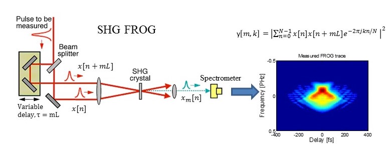 Figure 1
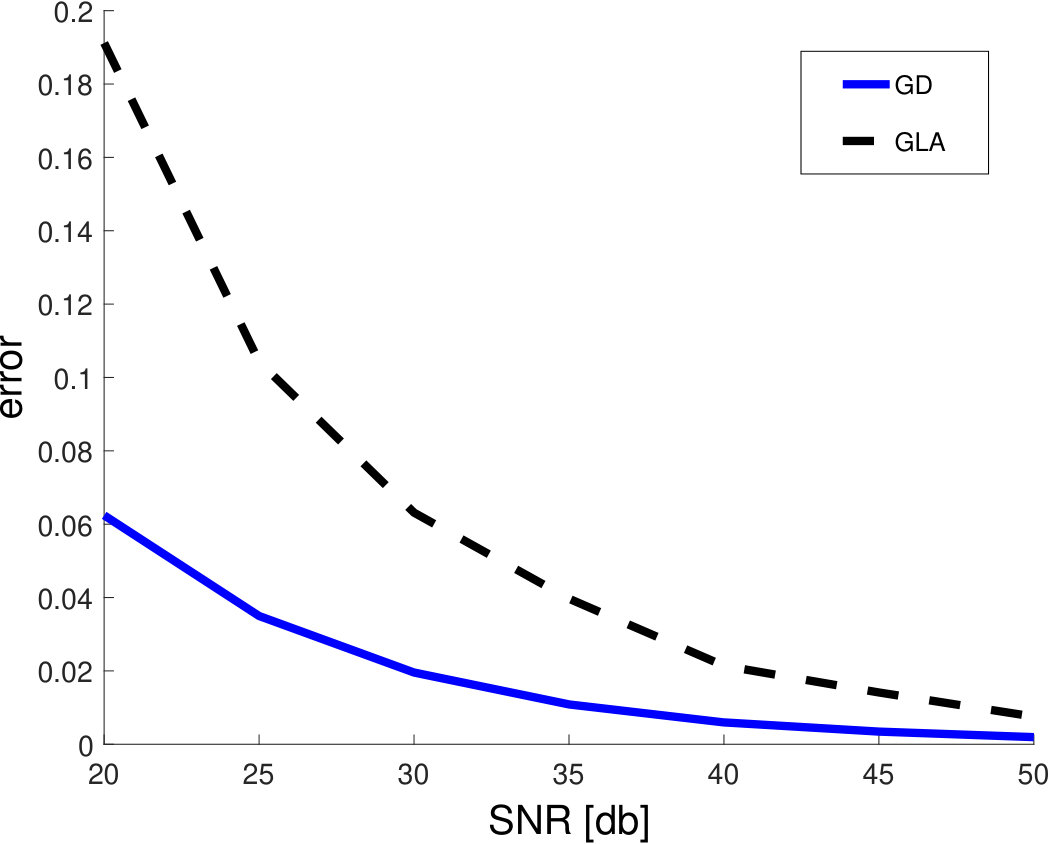 Figure 2
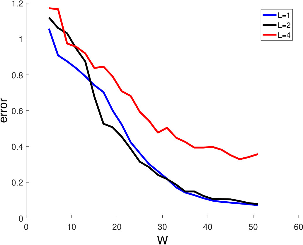 Figure 3
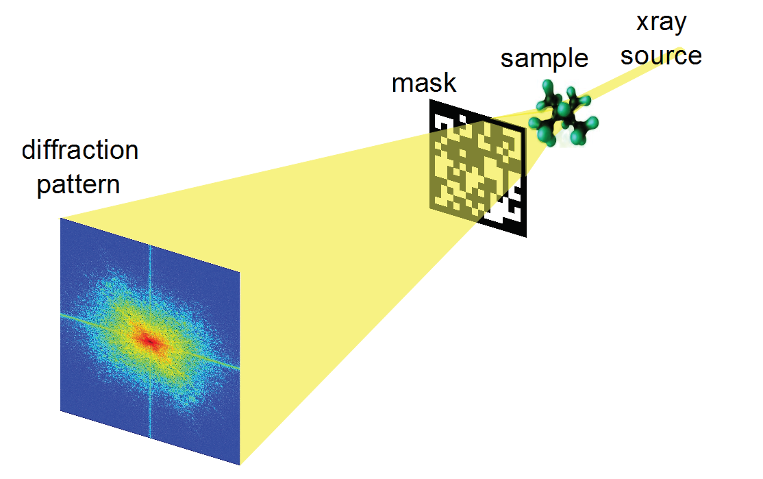 Figure 4
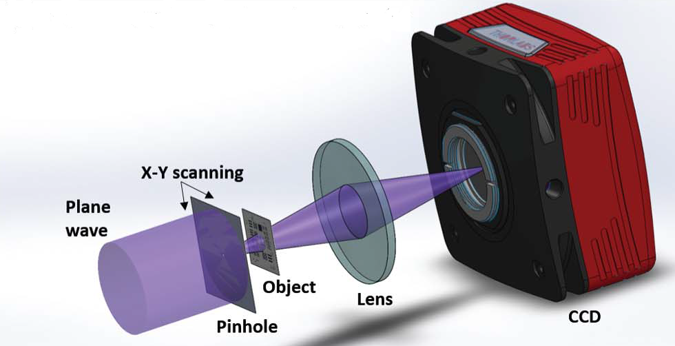 Figure 5
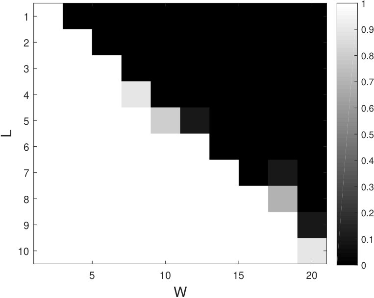 Figure 6
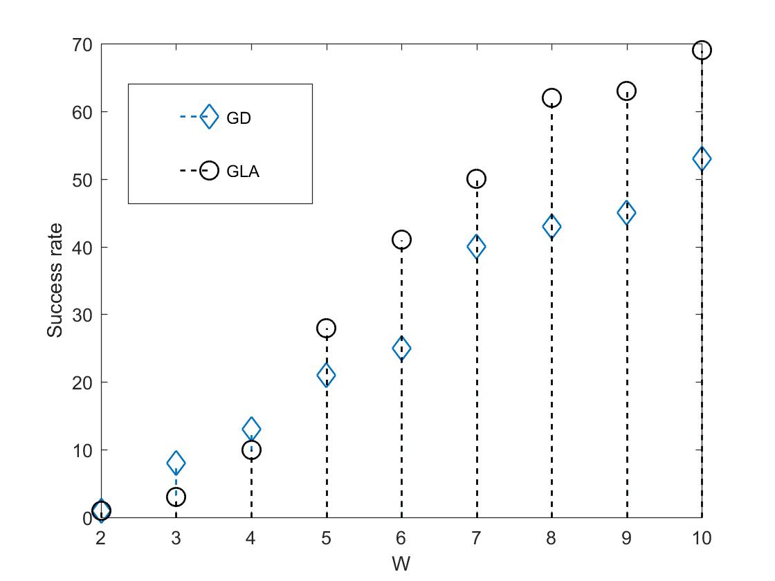 Figure 7
Peer Reviews
No public reviews on file for this paper yet. If you reviewed it on a platform where reviews are public (OpenReview, ICLR, NeurIPS, ICML), you can paste yours below so the community can read it here.
Videos
No videos yet. Explain this paper in a talk, walkthrough, or lecture? Add one.
Taxonomy
TopicsAdvanced X-ray Imaging Techniques
Fourier Phase Retrieval:
Uniqueness and Algorithms
Tamir Bendory [email protected] The Program in Applied and Computational Mathematics, Princeton University, Princeton, NJ, USA
Robert Beinert [email protected]. The Institute of Mathematics and Scientific Computing is a member of NAWI Graz (http://www.nawigraz.at). The author is supported by the Austrian Science Fund (FWF) within the project P 28858. Institute of Mathematics and Scientific Computing, University of Graz, Heinrichstraße 36, 8010 Graz, Austria
Yonina C. Eldar [email protected]. The author is supported by the European Union’s Horizon 2020 research and innovation program under grant agreement no. 646804-ERC-COG-BNYQ, and from the Israel Science Foundation under Grant no. 335/14. The Andrew and Erna Viterbi Faculty of Electrical Engineering, Technion - Israel Institute of Technology, Haifa, Israel
Abstract
The problem of recovering a signal from its phaseless Fourier transform measurements, called Fourier phase retrieval, arises in many applications in engineering and science. Fourier phase retrieval poses fundamental theoretical and algorithmic challenges. In general, there is no unique mapping between a one-dimensional signal and its Fourier magnitude and therefore the problem is ill-posed. Additionally, while almost all multidimensional signals are uniquely mapped to their Fourier magnitude, the performance of existing algorithms is generally not well-understood. In this chapter we survey methods to guarantee uniqueness in Fourier phase retrieval. We then present different algorithmic approaches to retrieve the signal in practice. We conclude by outlining some of the main open questions in this field.
1 Introduction
The task of recovering a signal from its Fourier transform magnitude, called Fourier phase retrieval, arises in many areas in engineering and science. The problem has a rich history, tracing back to 1952 [110]. Important examples for Fourier phase retrieval naturally appear in many optical settings since optical sensors, such as a charge-coupled device (CCD) and the human eye, are insensitive to phase information of the light wave. A typical example is coherent diffraction imaging (CDI) which is used in a variety of imaging techniques [24, 33, 34, 92, 105, 109]. In CDI, an object is illuminated with a coherent electro-magnetic wave and the far-field intensity diffraction pattern is measured. This pattern is proportional to the object’s Fourier transform and therefore the measured data is proportional to its Fourier magnitude. Phase retrieval also played a key role in the development of the DNA double helix model [55]. This discovery awarded Watson, Crick and Wilkins the Nobel prize in Physiology or Medicine in 1962 [1]. Additional examples for applications in which Fourier phase retrieval appear are X-ray crystallography, speech recognition, blind channel estimation, astronomy, computational biology, alignment and blind deconvolution [10, 19, 54, 62, 100, 114, 125, 132, 137].
Fourier phase retrieval has been a long-standing problem since it raises difficult challenges. In general, there is no unique mapping between a one-dimensional signal and its Fourier magnitude and therefore the problem is ill-posed. Additionally, while almost all multidimensional signals are uniquely mapped to their Fourier magnitude, the performance and stability of existing algorithms is generally not well-understood. In particular, it is not clear when given methods recover the true underlying signal. To simplify the mathematical analysis, in recent years attention has been devoted to a family of related problems, frequently called generalized phase retrieval. This refers to the setting in which the measurements are the phaseless inner products of the signal with known vectors. Particularly, the majority of works studied inner products with random vectors. Based on probabilistic considerations, a variety of convex and non-convex algorithms were suggested, equipped with stability guarantees from near-optimal number of measurements; see [3, 5, 30, 37, 44, 58, 124, 131, 133] to name a few works along these lines.
Here, we focus on the original Fourier phase retrieval problem and study it in detail. We begin by considering the ambiguities of Fourier phase retrieval [12, 15, 16]. We show that while in general a one-dimensional signal cannot be determined from its Fourier magnitude, there are several exceptional cases, such as minimum phase [66] and sparse signals [73, 101]. For general signals, one can guarantee uniqueness by taking multiple measurements, each one with a different mask. This setup is called masked phase retrieval [30, 69] and has several interesting special cases, such as the short-time Fourier transform (STFT) phase retrieval [22, 45, 71] and vectorial phase retrieval [82, 102, 103, 104]. For all aforementioned setups, we present algorithms and discuss their properties. We also study the closely–related Frequency-Resolved Optical Gating (FROG) methods [23] and multidimensional Fourier phase retrieval [78].
The outline of this chapter is as follows. In Section 2 we formulate the Fourier phase retrieval problem. We also introduce several of its variants, such as masked Fourier phase retrieval and STFT phase retrieval. In Section 3 we discuss the fundamental problem of uniqueness. Namely, conditions under which there is a unique mapping between a signal and its phaseless measurements. Section 4 is devoted to different algorithmic approaches to recover a signal from its phaseless measurements. Section 5 concludes the chapter and outlines some open questions. We hope that highlighting the gaps in the theory of phase retrieval will motivate more research on these issues.
2 Problem formulation
In this section, we formulate the Fourier phase retrieval problem and introduce notation.
Let be the underlying signal we wish to recover. In Fourier phase retrieval the measurements are given by
[TABLE]
Unless otherwise mentioned, we consider the over-sampled Fourier transform, i.e., , since in this case the acquired data is equivalent to the auto-correlation of as explained in Section 3.1. We refer to this case as the classical phase retrieval problem. As will be discussed in the next section, in general the classical phase retrieval problem is ill-posed. Nevertheless, some special structures may impose uniqueness. Two important examples are sparse signals obeying a non-periodic support [73, 101] and minimum phase signals [66]; see Section 3.2.
For general signals, a popular method to guarantee a unique mapping between the signal and its phaseless Fourier measurements is by utilizing several masks to introduce redundancy in the acquired data. In this case, the measurements are given by
[TABLE]
where are known masks. In matrix notation, this model can be written as
[TABLE]
where is the th row of the DFT matrix and is a diagonal matrix that contains the entries of the th mask. Classical phase retrieval is a special case in which and is the identity matrix.
There are several experimental techniques to generate masked Fourier measurements in optical setups [30]. One method is to insert a mask or a phase plate after the object [84]. Another possibility is to modulate the illuminating beam by an optical grating [85]. A third alternative is oblique illumination by illuminating beams hitting the object at specified angles [49]. An illustration of a masked phase retrieval setup is shown in Fig. 2.1.
An interesting special case of masked phase retrieval is signal reconstruction from phaseless STFT measurements. Here, all masks are translations of a reference mask, i.e., , where is a parameter that determines the overlapping factor between adjacent windows. Explicitly, the STFT phase retrieval problem takes on the form
[TABLE]
The reference mask is referred to as STFT window. We denote the length of the STFT window by , namely, for for some .
The problem of recovering a signal from its STFT magnitude arises in several applications in optics and speech processing. Particularly, it serves as the model of a popular variant of an ultra-short laser pulse measurement technique called Frequency-Resolved Optical Gating (FROG) which is introduced in Section 3.5 (the variant is referred to as X-FROG) [23, 127]. Another application is ptychography in which a moving probe (pinhole) is used to sense multiple diffraction measurements [87, 90, 106]. An illustration of a conventional ptychography setup is given in Fig. 2.2. A closely-related problem is Fourier ptychography [137].
The next section is devoted to the question of uniqueness. Namely, under what conditions on the signal and the masks there exists a unique mapping between the signal and the phaseless measurements. In Section 4 we survey different algorithmic approaches to recover the underlying signal from the acquired data.
3 Uniqueness guarantees
The aim of this section is to survey several approaches to ensure uniqueness of the discrete phase retrieval problem. We begin our study in Section 3.1 by considering the ambiguities arising in classical phase retrieval and provide a complete characterization of the solution set. Although the problem is highly ambiguous in general, uniqueness can be ensured if additional information about the signal is available. In Section 3.2, we first consider uniqueness guarantees based on the knowledge of the absolute value or phase of some signal entries. Next, we study sparse and minimum phase signals, which are uniquely defined by their Fourier magnitude and can be recovered by stable algorithms. In Sections 3.3 and 3.4 we show that for general signals, the ambiguities may be avoided by measuring the Fourier magnitudes of the interaction of the true signal with multiple deterministic masks or with several shifts of a fixed window. In Section 3.5 we study uniqueness guarantees for the closely–related FROG methods. Finally, in Section 3.6 we survey the multidimensional phase retrieval problems and their properties that differ significantly from the one-dimensional setting.
3.1 Trivial and non-trivial ambiguities
Considering the measurement model (LABEL:eq:PR_classical) of the classical phase retrieval problem, we immediately observe that the true signal cannot be recovered uniquely. For instance, the rotation (multiplication with a unimodular factor), the translation, or the conjugate reflection do not modify the Fourier magnitudes. Without further a priori constraints, the unknown signal is hence only determined up to these so-called trivial ambiguities, which are of minor interest. Beside the trivial ambiguities, the classical phase retrieval problem usually has a series of further non-trivial solutions, which can strongly differ from the true signal. For instance, the two non-trivially different signals
[TABLE]
yield the same Fourier magnitudes in (LABEL:eq:PR_classical); see [114].
To characterize the occurring non-trivial ambiguities, one can exploit the close relation between the given Fourier magnitudes with in (LABEL:eq:PR_classical) and the autocorrelation signal
[TABLE]
with for and , [15, 27]. For this purpose, we consider the product of the polynomial and the reversed polynomial , where denotes the polynomial with conjugate coefficients. Note that coincides with the usual -transform of the signal . Assuming that and , we have
[TABLE]
where is the autocorrelation polynomial of degree .
Since the Fourier magnitude (LABEL:eq:PR_classical) can be written as
[TABLE]
the autocorrelation polynomial is completely determined by the samples . The classical phase retrieval problem is thus equivalent to the recovery of from
[TABLE]
Comparing the roots of and , we observe that the roots of the autocorrelation polynomial occur in reflected pairs with respect to the unit circle. The main problem in the recovery of is now to decide whether or is a root of . On the basis of this observation, all ambiguities – trivial and non-trivial – are characterized in the following way.
Theorem 3.1**.**
[15]* Let be a complex-valued signal with and and with the Fourier magnitudes , , in (LABEL:eq:PR_classical). Then the polynomial of each signal with can be written as*
[TABLE]
where , and where is chosen from the reflected zero pairs of the autocorrelation polynomial . Moreover, up to of these solutions may be non-trivially different.
Since the support length of the true signal is directly encoded in the degree of the autocorrelation polynomial, all signals with in Theorem 3.1 have the same length, and the trivial shift ambiguity does not occur. The multiplication by is related to the trivial rotation ambiguity. The trivial conjugate reflection ambiguity is also covered by Theorem 3.1, since this corresponds to the reflection of all zeros at the unit circle and to an appropriate rotation of the whole signal. Hence, at least two of the possible zero sets always correspond to the same non-trivial solution, which implies that the number of non-trivial solutions of the classical phase retrieval problem is bounded by .
The actual number of non-trivial ambiguities for a specific phase retrieval problem, however, strongly depends on the zeros of the true solution. If denotes the number of zero pairs of the autocorrelation polynomial not lying on the unit circle, and the multiplicities of these zeros, then the different zero sets in Theorem 3.1 can consist of roots and roots , where is an integer between [math] and . Due to the trivial conjugation and reflection ambiguity, the corresponding phase retrieval problem has exactly
[TABLE]
non-trivial solutions [12, 51]. If, for instance, all zero pairs are unimodular, then the problem is even uniquely solvable.
3.2 Ensuring uniqueness in classical phase retrieval
To overcome the non-trivial ambiguities, and to ensure uniqueness in the phase retrieval problem, one can rely on suitable a priori conditions or further information about the true signal. For instance, if the sought signal represents an intensity or a probability distribution, then it has to be real-valued and non-negative. Unfortunately, this natural contraint does not guarantee uniqueness [13]. More appropriate priors like minimum phase or sparsity ensure uniqueness for almost every or, even, for every possible signal. Additional information about some entries of the true signal like the magnitude or the phase also guarantee uniqueness in certain settings.
3.2.1 Information about some entries of the true signal
One approach to overcome the non-trivial ambiguities is to use additional information about some entries of the otherwise unknown signal . For instance, in wave front sensing and laser optics [111], besides the Fourier intensity, the absolute values of the sought signal are available. Interestingly, already one absolute value within the support of the true signal almost always ensures uniqueness.
Theorem 3.2**.**
[16]* Let be an arbitrary integer between [math] and . Then almost every complex-valued signal with support length can be uniquely recovered from , , in (LABEL:eq:PR_classical) and up to rotations if . In the case , the reconstruction is almost surely unique up to rotations and conjugate reflections.*
The uniqueness guarantee in Theorem 3.2 cannot be improved by the knowledge of further or, even, all absolute values of the true signal. More precisely, one can explicitly construct signals that are not uniquely defined by their Fourier magnitudes and all temporal magnitudes for every possible signal length [16]. In order to recover a signal from its Fourier magnitudes and all temporal magnitudes numerically, several multi-level Gauss-Newton methods have been proposed in [79, 80, 111]. Under certain conditions, the convergence of these algorithms to the true solution is guaranteed, and they allow signal reconstruction from noise-free as well as from noisy data.
The main idea behind Theorem 3.2 exploits to show that the zero sets of signals that cannot be recovered uniquely (up to trivial ambiguities) form an algebraic variety of lesser dimension. This approach can be transferred to further kinds of information about some entries of . For instance, the knowledge of at least two phases of the true signal also guarantees uniqueness almost surely.
Theorem 3.3**.**
[16]* Let and be different integers in . Then almost every complex-valued signal with support length can be uniquely recovered from , , in (LABEL:eq:PR_classical), , and whenever . In the case , the recovery is only unique up to conjugate reflection except for and , where the set of non-trivial ambiguities is not reduced at all.*
As a consequence of Theorems 3.2 and 3.3, the classical phase retrieval problem is almost always uniquely solvable if at least one entry of the true signal is known. Unfortunately, there is no algorithm that knows how to exploit the given entries to recover the complete signal in a stable and efficient manner.
Corollary 3.4**.**
Let be an arbitrary integer between [math] and . Then almost every complex-valued signal with support length can be uniquely recovered from , , in (LABEL:eq:PR_classical) and if . In the case , the reconstruction is almost surely unique up to conjugate reflection.
Corollary 3.4 is a generalization of [136], where the recovery of real-valued signals from their Fourier magnitude and one of their end points or is studied. In contrast to Theorems 3.2 and 3.3, the classical phase retrieval problem becomes unique if enough entries of the true signal are known beforehand.
Theorem 3.5**.**
[15, 94]* Each complex-valued signal with signal length is uniquely determined by , , in (LABEL:eq:PR_classical) and the left end points .*
3.2.2 Sparse signals
In the last section, the true signal could be any arbitrary vector in . In the following, we consider the classical phase retrieval problem under the assumption that the unknown signal is sparse, namely, that only a small number of entries are non-zero. Sparse signals have been studied thoroughly in the last two decades, see for instance [32, 41, 43]. Phase retrieval problems of sparse signals arise in crystallography [76, 101] and astronomy [27, 101], for example. In many cases, the signal is sparse under an unknown transform. In the context of phase retrieval, a recent paper suggests a new technique to learn, directly from the phaseless data, the sparsifying transformation and the sparse representation of the signals simultaneously [126].
The union of all -sparse signals in , which have at most non-zero entries, is here denoted by . Since with is a -dimensional submanifold of and hence itself a Lebesgue null set, Theorem 3.2 and Corollary 3.4 cannot be employed to guarantee uniqueness of the sparse phase retrieval problem. Further, if the non-zero entries lie at equispaced positions within the true signal , i.e., the support is of the form for some positive integers and , this specific phase retrieval problem is equivalent to the recovery of a -dimensional vector from its Fourier intensity [73]. Due to the non-trivial ambiguities, which are characterized by Theorem 3.1, the assumed sparsity cannot always avoid non-trivial ambiguities.
In general, the knowledge that the true signal is sparse has a beneficial effect on the uniquness of phase retrieval. Under the restriction that the unknown signal belongs to the class of all -sparse signals in without equispaced support, which is again a -dimensional submanifold, the uniqueness is ensured for almost all signals.
Theorem 3.6**.**
[73]* Almost all signals can be uniquely recovered from their Fourier magnitudes , , in (LABEL:eq:PR_classical) up to rotations.*
Although Theorem 3.6 gives a theoretical uniqueness guarantee, it is generally a non-trivial task to decide whether a sparse signal is uniquely defined by its Fourier intensity. However, if the true signal does not possess any collisions, uniqueness is always given [101]. In this context, a sparse signal has a collision if there exists four indices , , , within the support of so that . A sparse signal without collisions is called collision-free. For instance, the signal
[TABLE]
is not collision-free since the index difference is equal to .
Theorem 3.7**.**
[101]* Assume that the signal with has no collisions.*
- •
If , then can be uniquely recovered from , , in (LABEL:eq:PR_classical) up to trivial ambiguities;
- •
If and not all non-zero entries have the same value, then can be uniquely recovered from , , in (LABEL:eq:PR_classical) up to trivial ambiguities;
- •
If and all non-zero entries have the same value, then can be uniquely recovered from , , in (LABEL:eq:PR_classical) almost surely up to trivial ambiguities.
The uniqueness guarantees in Theorem 3.7 remain valid for -sparse continuous-time signals, which are composed of pulses at arbitrary positions. More precisely, the continuous-time signal is here given by , where is the Dirac delta function, and . In this setting, the uniqueness can be guaranteed by samples of the Fourier magnitude [17].
In Section 4.4, we discuss different algorithms to recover sparse signals , that work well in practice.
3.2.3 Minimum phase signals
Based on the observation that each non-trivial solution of the classical phase retrieval problem is uniquely characterized by the zero set in Theorem 3.1, one of the simplest ideas to enforce uniqueness is to restrict these zeros in an appropriate manner. Under the assumption that the true signal is a minimum phase signal, which means that all zeros chosen from the reflected zero pairs of the autocorrelation polynomial lie inside the unit circle, the corresponding phase retrieval problem is uniquely solvable [64, 66].
Although the minimum phase constraint guarantees uniqueness, the question arises how to ensure that an unknown signal is minimum phase. Fortunately, each complex-valued signal may be augmented to a minimum phase signal.
Theorem 3.8**.**
[66]* For every , the augmented signal*
[TABLE]
with is a minimum phase signal.
Consequently, if the Fourier intensity of the augmented signal is available, then the true signal can always be uniquely recovered up to trivial ambiguities. Moreover, the minimum phase solution can be computed (up to rotations) from the Fourier magnitude as in (LABEL:eq:PR_classical) by a number of efficient algorithms [66]. Due to the trivial conjugate reflection ambiguity, this approach can be applied to maximum phase signals whose zeros lie outside the unit circle.
The minimum phase solution of a given phase retrieval problem may be determined in a stable manner using an approach by Kolmogorov [66]. For simplicity, we restrict ourselves to the real case with . The main idea is to determine the logarithm of the reversed polynomial from the given data . Under the assumption that all roots of strictly lie inside the unit circle, the analytic function may be written as
[TABLE]
where the unit circle is contained in the region of convergence. Substituting with , we have
[TABLE]
where and denote the real and imaginary parts, respectively. Since the real and imaginary part are a Hilbert transform pair, \Im\bigl{[}\log\tilde{X}(e^{-j\omega})\bigr{]} is completely defined by \Re\bigl{[}\log\tilde{X}(e^{-j\omega})\bigr{]}. Because of the identity , the real part may be computed from the autocorrelation polynomial by
[TABLE]
Finally, the autocorrelation polynomial is completely determined by the Fourier magnitudes , , leading to the recovery of the true minimum phase signal . Based on this idea, one can construct numerical algorithms that guarantee stable signal recovery under the presence of noise [66].
3.3 Phase retrieval with deterministic masks
A further possibility to obtain additional information about the underlying signal is to measure its Fourier magnitude with respect to different masks as described in (2.2) and (2.3). Assuming that the masks are constructed randomly, one can show that the corresponding phase retrieval problem has a unique solution up to rotations almost surely or, at least, with high probability. Depending on the random model, the number of employed masks to recover an one-dimensional signal varies form over to , see [6], [61], and [29] respectively. Moreover, in the multidimensional case, two independent masks are sufficient to guarantee uniqueness of almost every signal up to rotations [48]. As the following results show, in the deterministic setup, already a very small number of specifically constructed masks ensure uniqueness for most signals.
Theorem 3.9**.**
[69]* Almost all complex-valued signals can be uniquely recovered from , and , as in (2.2) up to rotations if the two masks , satisfy*
- •
* or for each ,*
- •
* for some .*
For some masks and , one can overcome the ‘almost all’ in Theorem 3.9 and obtain uniqueness of the corresponding phase retrieval problem.
Theorem 3.10**.**
[69]* If the diagonal matrices , correspond to the two masks*
[TABLE]
then every complex-valued signal with can be uniquely recovered from , and , up to rotations.
A different approach to exploit deterministic masks in order to overcome the ambiguity in phase retrieval is discussed in [72] and can be proven by using the characterization in Theorem 3.1. More explicitly, here the two masks
[TABLE]
for some between and are used. Pictorially, the mask blocks the right-hand side of the underlying signal and the left-hand side.
For the signals , , and , where is the diagonal matrix with respect to the mask , we define the polynomials , , and by
[TABLE]
Different from the autocorrelation functions of and , which are simply given by and , the autocorrelation function of the true signal can be written as
[TABLE]
since . Due to the fact that and have no common monomials with the same degree, one can determine the polynomials
[TABLE]
from the autocorrelation functions , and .
As mentioned before, the reversed polynomials correspond to the reflected zero set of with respect to the unit circle. Hence, assuming that the zeros of and are pairwise different, one can determine both zero sets by comparing the roots of the four polynomials (3.3), which yields the following result.
Theorem 3.11**.**
[72]* Let , and assume that the zeros and of*
[TABLE]
are pairwise different. Then the signal can be uniquely recovered up to rotations from the Fourier magnitudes , and , with the masks and , in (3.2).
The phase retrieval problem in Theorem 3.11 is equivalent to the recovery of and with support and from the Fourier magnitudes of , , and . More generally, the recovery of two arbitrary signals , from their Fourier magnitudes and the Fourier magnitude of the interference has been studied in [15, 77]. Theorem 3.11 is a specific instance of the uniqueness guarantee given in [15]. Furthermore, these problems are closely related to the vectorial phase retrieval problem introduced in [81, 102, 104], where the Fourier magnitudes of a second interference are employed.
A further example for phase retrieval with deterministic masks is considered in [30], where the three masks are defined by
[TABLE]
for a non-negative integer . The masks and here interfere the unknown signal with a modulated version of the unknown signal itself, which yields the Fourier magnitudes and . Together with the Fourier magnitudes , for almost every signal, the relative phases of the Fourier transform can be determined. If is relatively prime with , then the Fourier transform and thus the true signal are recovered up to rotations.
Theorem 3.12**.**
[30]* Let be a signal with non-vanishing DFT. Then is uniquely recovered from with and the masks in (3.4) up to rotations if and only if the non-negative integer is relatively prime with .*
The masks in (3.4) as well as the uniqueness guarantee in Theorem 3.12 can be generalized to multidimensional phase retrieval [30]. If is replaced by , every signal is uniquely recovered up to rotation from its Fourier magnitudes in (2.2) with masks and , , where , and where can be nearly every real number [14]. Several further examples of deterministic masks which allow a unique recovery are detailed in [14, 30, 69, 72] and references therein. In Section 4.2, we consider semidefinite relaxation algorithms which stably recover the unknown signal from its masked Fourier magnitudes (2.2) under noise.
3.4 Phase retrieval from STFT measurements
We next consider uniqueness guarantees for the recovery of an unknown signal from the magnitude of its STFT as defined in (2.4). This problem can be interpreted as a sequence of classical phase retrieval problems, where some entries of the underlying signals have to coincide. Obviously, the STFT phase retrieval problem cannot be solved uniquely if the parameter is greater than or equal to the window length , since the classical problems are then independent from each other.
Under the assumption that the known window does not vanish, i.e., for , some of the first uniqueness guarantees were established in [94].
Theorem 3.13**.**
[94]* Let be a non-vanishing window of length , and let be an integer in . If the signal with support length has at most consecutive zeros between any two non-zero entries, and if the first entries of are known, then can be uniquely recovered from with in (2.4).*
The main idea behind Theorem 3.13 is that the corresponding classical phase retrieval problems are solved sequentially. For instance, the case is equivalent to recovering a signal in from its Fourier intensity and the first entries. The uniqueness of this phase retrieval problem is guaranteed by Theorem 3.5. Since the true signal has at most consecutive zeros, the remaining subproblems can also be reduced to the setting considered in Theorem 3.5.
Knowledge of the first entries of in Theorem 3.13 is a strong restriction in practice. Under the a priori constraint that the unknown signal is non-vanishing everywhere, the first entries are not needed to ensure uniqueness.
Theorem 3.14**.**
[71]* Let be a non-vanishing window of length satisfying . Then almost all non-vanishing signals can be uniquely recovered up to rotations from their STFT magnitudes in (2.4) with and .*
For some classes of STFT windows, the uniqueness is guaranteed for all non-vanishing signals [22, 45]. Both references use a slightly different definition of the STFT, where the STFT window in (2.4) is periodically extended over the support , i.e., the indices of the window are considered as modulo the signal length .
Theorem 3.15**.**
[45]* Let be a periodic window with support length and , and assume that the length- DFT of is non-vanishing. If and are co-prime, then every non-vanishing signal can be uniquely recovered from its STFT magnitudes in (2.4) with and up to rotations.*
Theorem 3.16**.**
[22]* Let be a periodic window of length , and assume that the length- DFT of and are non-vanishing. Then every non-vanishing signal can be uniquely recovered from its STFT magnitudes in (2.4) with and up to rotations.*
If we abandon the constraint that the underlying signal is non-vanishing, then the behaviour of the STFT phase retrieval problem changes dramatically, and the recovery of the unknown signal becomes much more challenging. For example, if the unknown signal possesses more than consecutive zero entries, then the signal can be divided in two parts, whose STFTs are completely independent. An explicit non-trivial ambiguity for this specific setting is constructed in [45]. Depending on the window length, there are thus some natural limitations on how far uniqueness can be ensured for sparse signals.
Theorem 3.17**.**
[71]* Let be a non-vanishing window of length satisfying . Then almost all sparse signals with less than consecutive zeros can be uniquely recovered up to rotations from their STFT magnitudes in (2.4) with and .*
In [25], the STFT is interpreted as measurements with respect to a Gabor frame. Under certain conditions on the generator of the frame, every signal is uniquely recovered up to rotations. Further, the true signal is given as a closed form solution. For the STFT model in (2.4), this implies the following uniqueness guarantee.
Theorem 3.18**.**
[25]* Let be a periodic window of length , and assume that the length- DFT of is non-vanishing for . Then every signal can be uniquely recovered from its STFT magnitudes in (2.4) with and up to rotations.*
The main difference between Theorem 3.18 and the uniqueness results before is that the unknown signal can have arbitrarily many consecutive zeros. On the other hand, the STFT window must have a length of at least in order to ensure that is not the zero vector. Thus, the thm is only relevant for long windows. A similar result was derived in [22], followed by a stable recovery algorithm; see Section 4.3.
3.5 FROG methods
An important optical application for phase retrieval is ultra-short laser pulse characterization [127, 128]. One way to overcome the non-uniqueness of Fourier phase retrieval in this application is by employing a measurement technique called X-FROG (see also Section 2). In X-FROG, a reference window is used to gate the sought signal, resulting in the STFT phase retrieval model (2.4). However, in practice it is quite hard to generate and measure such a reference window. Therefore, in order to generate redundancy in ultra-short laser pulse measurements it is common to correlate the signal with itself. This method is called Frequency-Resolved Optical Gating (FROG).
FROG is probably the most commonly used approach for full characterization of ultra-short optical pulses due to its simplicity and good experimental performance. A FROG apparatus produces a 2D intensity diagram of an input pulse by interacting the pulse with delayed versions of itself in a nonlinear-optical medium, usually using a second harmonic generation (SHG) crystal [40]. This 2D signal is called a FROG trace and is a quartic function of the unknown signal. An illustration of the FROG setup is presented in Fig. 3.1. Here we focus on SHG FROG but other types of nonlinearities exist for FROG measurements. A generalization of FROG, in which two different unknown pulses gate each other in a nonlinear medium, is called blind FROG. This method can be used to characterize simultaneously two signals [135]. In this case, the measured data is referred to as a blind FROG trace and is quadratic in both signals. We refer to the problems of recovering a signal from its blind FROG trace and FROG trace as bivariate phase retrieval and quartic phase retrieval, respectively.
In bivariate phase retrieval we acquire, for each delay step , the power spectrum of
[TABLE]
where , as in the STFT phase retrieval setup, determines the overlap factor between adjacent sections. The acquired data is given by
[TABLE]
Quartic phase retrieval is the special case in which .
The trivial ambiguities of bivariate phase retrieval are described in the following proposition.
Proposition 3.19**.**
[23]* Let and let for some fixed . Then, the following signals have the same phaseless bivariate measurements as the pair :*
multiplication by global phases for some , 2. 2.
the shifted signal for some , 3. 3.
the conjugated and reflected signal , 4. 4.
modulation, , for some .
The fundamental question of uniqueness for FROG methods has been analyzed first in [112] for the continuous setup. The analysis of the discrete setup appears in [23].
Theorem 3.20**.**
[23]* Let , and let and be the Fourier transforms of and , respectively. Assume that has at least consecutive zeros (e.g., band-limited signal). Then, almost all signals are determined uniquely, up to trivial ambiguities, from the measurements in (3.5) and the knowledge of and . By trivial ambiguities we mean that and are determined up to global phase, time shift and conjugate reflection.*
Several heuristic techniques have been proposed to estimate an underlying signal from its FROG trace. These algorithms are based on a variety of methods, such as alternating projections, gradient descent and iterative PCA [75, 121, 129].
3.6 Multidimensional phase retrieval
In a wide range of real-world applications like crystallography or electron microscopy, the natural objects of interest correspond to two or three-dimensional signals. More generally, the -dimensional phase retrieval problem consists of the recovery of an unknown -dimensional signal from its Fourier magnitudes
[TABLE]
with and . Unless otherwise mentioned, we assume .
Clearly, rotations, transitions, or conjugate reflections of the true signal lead to trivial ambiguities. Besides these similarities, the ambiguities of the multidimensional phase retrieval problem are very different from those of its one-dimensional counterpart. More precisely, non-trivial ambiguities occur only in very rare cases, and almost every signal is uniquely defined by its Fourier magnitude up to trivial ambiguities.
Similarly to Section 3.1, the non-trivial ambiguities can be characterized by exploiting the autocorrelation. Here the related polynomial
[TABLE]
with is uniquely factorized (up to multiplicative constants) into irreducible factors , which means that the cannot be represented as a product of multivariate polynomials of lesser degree. The main difference with the one-dimensional setup is that most multivariate polynomials consists of only one irreducible factor . Denoting the multivariate reversed polynomial by
[TABLE]
with , where is the degree of with respect to the variable , the non-trivial ambiguities in the multidimensional setting are characterized as follows.
Theorem 3.21**.**
[63]* Let be the complex-valued signal related to the polynomial , where are non-trivial irreducible polynomials. Then the polynomial of each signal with Fourier magnitudes in (3.6) can be written as*
[TABLE]
for some index set .
Thus, the phase retrieval problem is uniquely solvable up to trivial ambiguities if the algebraic polynomial of the true signal is irreducible, or if all but one factor are invariant under reversion [63]. In contrast to the one-dimensional case, where the polynomial may always be factorized into linear factors with respect to the zeros , cf. Theorem 3.1, most multivariate polynomials cannot be factorized as mentioned above.
Theorem 3.22**.**
[65]* The subset of the -variate polynomials with of degree in which are reducible over the complex numbers corresponds to a set of measure zero.*
Consequently, the multidimensional phase retrieval problem has a completely different behaviour than its one-dimensional counterpart.
Corollary 3.23**.**
Almost every -dimensional signal with is uniquely defined by its Fourier magnitudes in (3.6) up to trivial ambiguities.
Investigating the close connection between the one-dimensional and two-dimensional problem formulations, the different uniqueness properties have been studied in [78]. Particularly, one can show that the two-dimensional phase retrieval problem corresponds to a one-dimensional problem with additional constraints, which almost always guarantee uniqueness. Despite these uniqueness guarantees, there are no systematic methods to estimate an -dimensional signal from its Fourier magnitude [8, 78]. The most popular techniques are based on alternating projection algorithms as discussed in Section 4.1.
4 Phase retrieval algorithms
The previous section presented conditions under which there exists a unique mapping between a signal and its Fourier magnitude (up to trivial ambiguities). Yet, the existence of a unique mapping does not imply that we can actually estimate the signal in a stable fashion. The goal of this section is to present different algorithmic approaches for the inverse problem of recovering a signal from its phaseless Fourier measurements. In the absence of noise, this task can be formulated as a feasibility problem over a non-convex set
[TABLE]
Recall that (4.1) covers the classical and STFT phase retrieval problems as special cases.
From the algorithmic point–of–view, it is often more convenient to formulate the problem as a minimization problem. Two common approaches are to minimize the intensity–based loss function
[TABLE]
or the amplitude–based loss function (see for instance [52, 133, 130])
[TABLE]
The chief difficulty arises from the non-convexity of these loss functions. For example, if is a real signal, then (4.2) is a sum of quartic polynomials. Hence, there is no reason to believe that a gradient algorithm will converge to the target signal from an arbitrary initialization. To demonstrate this behavior, we consider an STFT phase retrieval setup for which a unique solution is guaranteed (see Theorem 3.16). We attempt to recover the signal by employing two methods: a gradient descent algorithm that minimizes (4.2) and the classical Griffin-Lim algorithm (see Section 4.1 and Algorithm 2). Both techniques were initialized from 100 different random vectors. As can be seen in Fig. 4.1, even for long windows, the algorithms do not always converge to the global minimum. Furthermore, the success rate decreases with the window’s length. In what follows, we present different systematic approaches to recover a signal from its phaseless Fourier measurements and discuss their advantages and shortcomings.
The rest of this section is organized as follows. We begin in Section 4.1 by introducing the classical algorithms which are based on alternating projections. Then, we proceed in Section 4.2 with convex programs based on semidefinite programming (SDP) relaxations. SDPs have gained popularity in recent years as they provide good numerical performance and theoretical guarantees. We present SDP-based algorithms for masked phase retrieval, STFT phase retrieval, minimum phase and sparse signals. In Section 4.3, we survey additional non-convex algorithms with special focus on STFT phase retrieval. Section 4.4 presents several algorithms specialized for the case of phase retrieval of sparse signals.
4.1 Alternating projection algorithms
In their seminal work [56], Gerchberg and Saxton considered the problem of recovering a signal from its Fourier and temporal magnitude. They proposed an intuitive solution which iterates between two basic steps. The algorithm begins with an arbitrary initial guess. Then, at each iteration, it imposes the known Fourier magnitude and temporal magnitude consecutively. This process proceeds until a stopping criterion is attained.
The basic concept of the Gerchberg-Saxton algorithm was extended by Fienup in 1982 to a variety of phase retrieval settings [52, 53]. Fienup suggested to replace the temporal magnitude constraint by other alternative constraints in the time domain. Examples for such constraints are the knowledge of the signal’s support or few entries of the signal, non-negativity, or a known subspace in which the signal lies. Recently, it was also suggested to incorporate sparsity priors [93]. These algorithms have the desired property of error reduction. Let be the Fourier transform of the estimation in the th iteration. Then, it can be shown that the quantity is monotonically non-increasing. This class of methods is best understood as alternating projection algorithms [46, 89, 97]. Namely, each iteration consists of two consecutive projections onto sets defined by the spectral and temporal constraints. As the first step projects onto a non-convex set (and in some cases, the temporal projection is non-convex as well) the iterations may not converge to the target signal. The method is summarized in Algorithm 1, where we use the definition
[TABLE]
Over the years, many variants of the basic alternating projection scheme have been suggested. A popular algorithm used for CDI applications is the hybrid input-output (HIO), which consists of an additional correction step in the time domain [52]. Specifically, the last stage of each iteration is of the form
[TABLE]
where is the set of indices for which violates the temporal constraint (e.g., support constraint, non-negativity) and is a small parameter. While there is no proof that the HIO converges, it tends to avoid local minima in the absence of noise. Additionally, it is known to be sensitive to the prior knowledge accuracy [114]. For additional alternating projection schemes, we refer the interested reader to [9, 35, 47, 86, 91, 107].
Griffin and Lim proposed a modification of Algorithm 1 specialized for STFT phase retrieval [60]. In this approach, the last step at each iteration harnesses the knowledge of the STFT window to update the signal estimation. The Griffin-Lim heuristic is summarized in Algorithm 2.
4.2 Semidefinite relaxation algorithms
In recent years, algorithms based on convex relaxation techniques have attracted considerable attention [30, 131]. These methods are based on the insight that while the feasibility problem (4.1) is quadratic with respect to , it is linear in the matrix . This leads to a natural convex SDP relaxation that can be solved in polynomial time using standard solvers like CVX [59]. In many cases, these relaxations achieve excellent numerical performance followed by theoretical guarantees. However, the SDP relaxation optimizes over variables and therefore its computational complexity is quite high.
SDP relaxation techniques begin by reformulating the measurement model (2.3) as a linear function of the Hermitian rank–one matrix :
[TABLE]
Consequently, the problem of recovering from can be posed as the feasibility problem of finding a rank–one Hermitian matrix which is consistent with the measurements:
[TABLE]
where is the set of all Hermitian matrices. If there exists a matrix satisfying all the constraints of (4.4), then it determines up to global phase. The feasibility problem (4.4) is non-convex due to the rank constraint. A convex relaxation may be obtained by omitting the rank constraint leading to the SDP [30, 57, 116, 131]:
[TABLE]
If the solution of (4.5) happens to be of rank one, then it determines up to global phase. In practice, it is useful to promote a low rank solution by minimizing an objective function over the constraints of (4.5). A typical choice is the trace function, which is the convex hull of the rank function for Hermitian matrices. The resulting SDP relaxation algorithm is summarized in Algorithm 3.
The SDP relaxation for the classical phase retrieval problem (i.e., and ) was investigated in [66]. It was shown that SDP relaxation achieves the optimal cost function value of (4.2). However, recall that in general the classical phase retrieval problem does not admit a unique solution. Minimum phase signals are an exception as explained in Section 3.2.3. Let be the autocorrelation sequence of the estimated signal from Algorithm 3. If is minimum phase, then it can be recovered by the following program:
[TABLE]
where is a Toeplitz matrix with ones in the th diagonal and zero otherwise. The solution of (4.6), , is guaranteed to be rank one so that . See Section 3.2.3 for a different algorithm to recover minimum phase signals.
An SDP relaxation for deterministic masks was investigated in [69], where the authors consider two types of masks. Here, we consider the two masks, and given in (3.1). Let and be the diagonal matrices associated with and , respectively, and assume that each measurement is contaminated by bounded noise . Then, it was suggested to estimate the signal by solving the following convex program
[TABLE]
This program achieves stable recovery in the sense that the recovery error is proportional to the noise level and reduces to zero in the noise-free case. Note however that in the presence of noise the solution is not likely to be rank one.
Theorem 4.1**.**
[69]* Consider a signal satisfying and . Suppose that the measurements are taken with the diagonal matrices and (masks) associated with and given in (3.1). Then, the solution of the convex program (4.7) obeys*
[TABLE]
for some numerical constant .
Phase retrieval from STFT measurements using SDP was considered in [71]. Here, SDP relaxation in the noiseless case takes on the form
[TABLE]
where is the number of STFT windows and (see (2.4)). In [71], it was proven that (4.8) recovers the signal exactly under the following conditions.
Theorem 4.2**.**
[71]* The convex program (4.8) has a unique feasible matrix for almost all non-vanishing signals if:*
- •
* for ,*
- •
,
- •
,
- •
* is known apriori for ,*
where is the window’s length.
Note that for no prior knowledge on the entries of is required.
An interesting implication of this thm is that recovery remains exact even if we merely have access to the low frequencies of the data. This property is called super-resolution and will be discussed in more detail in the context of sparse signals. Numerically, the performance of (4.8) is better than Theorem 4.2 suggests. Specifically, it seems that for , (4.8) recovers exactly without any prior knowledge on the entries of , as demonstrated in Fig. 4.2 (a similar example is given in [71]). Additionally, the program is stable in the presence of noise.
4.3 Additional non-convex algorithms
In this section, we present additional non-convex algorithms for phase retrieval with special focus on STFT phase retrieval. A naive way to estimate the signal from its phaseless measurements is by minimizing the non-convex loss functions (4.2) or (4.3) by employing a gradient descent scheme. However, as demonstrated in Fig. 4.1, this algorithm is likely to converge to a local minimum due to the non-convexity of the loss functions. Hence, the key is to introduce an efficient method to initialize the non-convex algorithm sufficiently close to the global minimum.
A recent paper [22] suggests an initialization technique for STFT phase retrieval, which we now describe. Consider the one-dimensional Fourier transform of the data with respect to the frequency variable (see (2.4)), given by
[TABLE]
where and both the signal and the window are assumed to be periodic. For fixed , we obtain the linear system of equations
[TABLE]
where , is the th diagonal of the matrix and is the matrix with th entry given by . For , is a circulant matrix. Clearly, recovering for all is equivalent to recovering . Hence, the ability to estimate depends on the properties of the window which determines . To make this statement precise, we use the following definition.
Definition 4.3**.**
A window is called an admissible window of length if for all the associated circulant matrices in (4.9) are invertible.
An example of an admissible window is a rectangular window with and a prime number. If the STFT window is sufficiently long and admissible, then the STFT phase retrieval has a closed-form solution. This solution can be obtained by the principal eigenvector of a matrix, constructed as the solution of a least-squares problem according to (4.9). This algorithm is summarized in Algorithm 4.
Theorem 4.4**.**
[22]* Let and suppose that is an admissible window of length (see Definition 4.3). Then, Algorithm 4 recovers any complex signal up to global phase.*
In many cases, the window is shorter than . However, the same technique can be applied to initialize a refinement process, such as a gradient method or the Griffin-Lim algorithm (GLA). In this case, the distance between the initial vector (the output of Algorithm 4) and the target signal can be estimated as follows.
Theorem 4.5**.**
[22]* Suppose that , , is an admissible window of length and that for some . Then, the output of Algorithm 4 satisfies*
[TABLE]
For , it is harder to obtain a reliable estimation of the diagonals of . Nevertheless, a simple heuristic is proposed in [22] based on the smoothing properties of typical STFT windows. Fig. 4.3 shows experiments corroborating the effectiveness of this initialization approach for .
We have seen that under some conditions, the STFT phaseless measurements provide partial information on the matrix . In some cases, the main diagonal of , or equivalently the temporal magnitude of , are also measured. Therefore, if the signal is non-vanishing, then all entries of the matrix can be normalized to have unit modulus. This in turn implies that the STFT phase retrieval problem is equivalent to estimating the missing entries of a rank–one matrix with unit modulus entries (i.e., phases). This problem is known as phase synchronization. In recent years, several algorithms for phase synchronization were suggested and analyzed, among them eigenvector-based methods, SDP relaxations, projected power methods and approximate message passing algorithms [4, 7, 26, 36, 98, 122]. Recent papers [67, 68] adopted this approach and suggested spectral and greedy algorithms for STFT phase retrieval. These methods are accompanied by stability guarantees and can be modified for phase retrieval using masks. The main shortcoming of this approach is that it relies on a good estimation of the temporal magnitudes which may not always be available.
Another interesting approach has been recently proposed in [99]. This paper suggests a multi-stage algorithm based on spectral clustering and angular synchronization. It is shown that the algorithm achieves stable estimation (and exactness in the noise-free setting) with only phaseless STFT measurements. Nevertheless, the algorithm builds upon random STFT windows of length while most applications use shorter windows.
4.4 Algorithms for sparse signals
In this section, we assume that the signal is sparse with a sparsity level defined as
[TABLE]
In this case, the basic phase retrieval problem (4.2) can be modified to the constrained least-squares problem
[TABLE]
where we use as the standard pseudo-norm counting the non-zero entries of a signal.
Many phase retrieval algorithms for sparse signals are modifications of known algorithms for the non-sparse case. For instance, gradient algorithms where modified to take into account the sparsity structure. The underlying idea of these algorithms is to add a thresholding step at each iteration. Theoretical analysis of these algorithms for phase retrieval with random sensing vectors is considered in [28, 134]. A similar modification for the HIO algorithm was proposed in [93]. Modifications of SDP relaxation methods for phase retrieval with random sensing vectors were considered in [83, 95, 96]. Here, the core idea is to incorporate a sparse-promoting regularizer in the objective function. However, this technique cannot be adapted directly to Fourier phase retrieval because of the trivial ambiguities of translation and conjugate reflection; see a detailed explanation in [70]. To overcome this barrier, a Two-Stage Sparse Phase-Retrieval (TSPR) algorithm was proposed in [73]. The first stage of the algorithm involves estimating the support of the signal directly from the support of its autocorrelation. This problem is equivalent to the turnpike problem of estimating a set of integers from their pairwise distances [123]. Once the support is known, the second stage involves solving an SDP to estimate the missing amplitudes. It was proven that TSPR recovers signals exactly in the noiseless case as long as the sparsity level is less than . In the noisy setting, recovery is robust for sparsity level lower than . A different SDP-based approach was suggested in [116]. This method proposes to promote a sparse solution by the log-det heuristic [50] and an constraint on the matrix .
An alternative class of algorithms that has been proven to be highly effective for sparse signals is the class of greedy algorithms, see for instance [11, 88]. For phase retrieval tasks, a greedy optimization algorithm called GESPAR (GrEedy Sparse PhAse Retrieval) is proposed in [113]. The algorithm was applied for a variety of optical tasks, such as CDI and phase retrieval through waveguide arrays [115, 117, 119, 120]. GESPAR is a local search algorithm, based on iteratively updating the signal support. Specifically, two elements are being updated at each iteration by swapping. Then, a non-convex objective function that takes the support into account is minimized by a damped Gauss-Newton method. The swap is carried out between the support element corresponds to the smallest entry (in absolute value) and the off-support element with maximal gradient value of the objective function. A modification of GESPAR for STFT phase retrieval was presented in [45]. A schematic outline of GESPAR is given in Algorithm 5; for more details, see [113].
In practice, many optical measurement processes blur the fine details of the acquired data and act as low-pass filters. In these cases, one aims at estimating the signal from its low-resolution Fourier magnitudes. This problem combines two classical problems: phase retrieval and super-resolution. In recent years, super-resolution for sparse signals has been investigated thoroughly [2, 18, 20, 21, 31, 42]. In Theorem 4.2, we have seen that the SDP (4.8) can recover a signal from its low-resolution STFT magnitude. The problem of recovering a signal from its low-resolution phaseless measurements using masks was considered in [74, 108]. It was proven that exact recovery may be obtained by only few111Specifically, several combinations of masks are suggested. Each combination consists of three to five deterministic masks. carefully designed masks if the underlying signal is sparse and its support is not clustered (this requirement is also known as the separation condition). An extension to the continuous setup was suggested in [39]. A combinatorial algorithm for recovering a signal from its low-resolution Fourier magnitude was suggested in [38]. The algorithm recovers an -sparse signal exactly from low-pass magnitudes. Nevertheless, this algorithm is unstable in the presence of noise due to error propagation.
5 Conclusion
In this chapter, we studied the problem of Fourier phase retrieval. We focused on the question of uniqueness, presented the main algorithmic approaches and discussed their properties. To conclude the chapter, we outline several fundamental gaps in the theory of Fourier phase retrieval.
Although many different methods have been proposed and analyzed in the last decade for Fourier phase retrieval, alternating projection algorithms maintained their popularity. Nevertheless, the theoretical understanding of these algorithms is limited. Another fundamental open question regards multidimensional phase retrieval. While almost all multidimensional signals are determined uniquely by their Fourier magnitude, there is no method that provably recovers the signal.
In many applications in optics, the measurement process acts as a low-pass filter. Hence, a practical algorithm should recover the missing phases (phase retrieval) and resolve the fine details of the data (super-resolution). In this chapter, we surveyed several works dealing with the combined problem. Nonetheless, the current approaches are based on inefficient SDP programs [39, 71, 74, 108] or lack theoretical analysis [22, 116]. Additionally, even if all frequencies are available, it is still not clear what is the maximal sparsity that enables efficient and stable recovery of a signal from its Fourier magnitude.
In ultra short laser pulse characterization, it is common to use the FROG methods that were introduced in Section 3.5. It is interesting to understand the minimal number of measurements which can guarantee uniqueness for FROG-type methods. Additionally, a variety of algorithms are applied to estimate signals from FROG-type measurements; a theoretical understanding of these algorithms is required.
The reference list from the paper itself. Each links out to its DOI / PubMed record.
- 1[1] https://www.nobelprize.org/nobel_prizes/medicine/laureates/1962/ .
- 2[2] Jean-Marc Azais, Yohann De Castro, and Fabrice Gamboa. Spike detection from inaccurate samplings. Applied and Computational Harmonic Analysis , 38(2):177–195, 2015.
- 3[3] Radu Balan, Pete Casazza, and Dan Edidin. On signal reconstruction without phase. Applied and Computational Harmonic Analysis , 20(3):345–356, 2006.
- 4[4] Afonso S. Bandeira, Nicolas Boumal, and Amit Singer. Tightness of the maximum likelihood semidefinite relaxation for angular synchronization. Mathematical Programming , 163(1):145–167, 2017.
- 5[5] Afonso S Bandeira, Jameson Cahill, Dustin G Mixon, and Aaron A Nelson. Saving phase: Injectivity and stability for phase retrieval. Applied and Computational Harmonic Analysis , 37(1):106–125, 2014.
- 6[6] Afonso S Bandeira, Yutong Chen, and Dustin G Mixon. Phase retrieval from power spectra of masked signals. Information and Interference: A Journal of the IMA , 3(2):83–102, 2014.
- 7[7] Afonso S Bandeira, Yutong Chen, and Amit Singer. Non-unique games over compact groups and orientation estimation in cryo-em. ar Xiv preprint ar Xiv:1505.03840 , 2015.
- 8[8] Heinz H Bauschke, Patrick L Combettes, and D Russell Luke. Phase retrieval, error reduction algorithm, and fienup variants: a view from convex optimization. JOSA A , 19(7):1334–1345, 2002.