An Inverse Problem for Infinitely Divisible Moving Average Random Fields
Wolfgang Karcher, Stefan Roth, Evgeny Spodarev, Corinna Walk

TL;DR
This paper addresses the nonparametric estimation of Lévy characteristics in infinitely divisible moving average random fields using three different methods, providing theoretical error bounds and simulation comparisons.
Contribution
It introduces three novel estimation methods for Lévy densities in random fields and analyzes their theoretical performance and practical effectiveness.
Findings
All three methods provide consistent $L^2$-error bounds.
Numerical simulations compare the performance of the methods.
The Fourier-based approach shows promising accuracy in simulations.
Abstract
Given a low frequency sample of an infinitely divisible moving average random field with a known simple function , we study the problem of nonparametric estimation of the L\'{e}vy characteristics of the independently scattered random measure . We provide three methods, a simple plug-in approach, a method based on Fourier transforms and an approach involving decompositions with respect to -orthonormal bases, which allow to estimate the L\'{e}vy density of . For these methods, the bounds for the -error are given. Their numerical performance is compared in a simulation study.
Click any figure to enlarge with its caption.
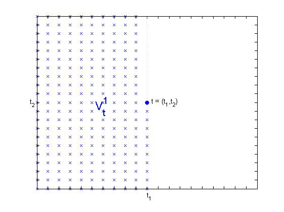 Figure 1
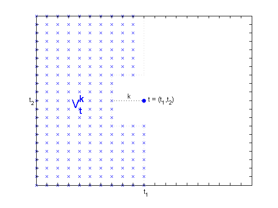 Figure 2
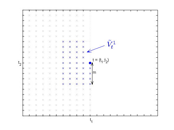 Figure 3
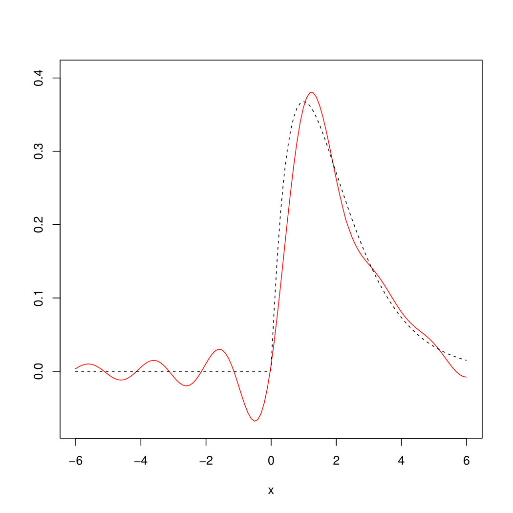 Figure 4
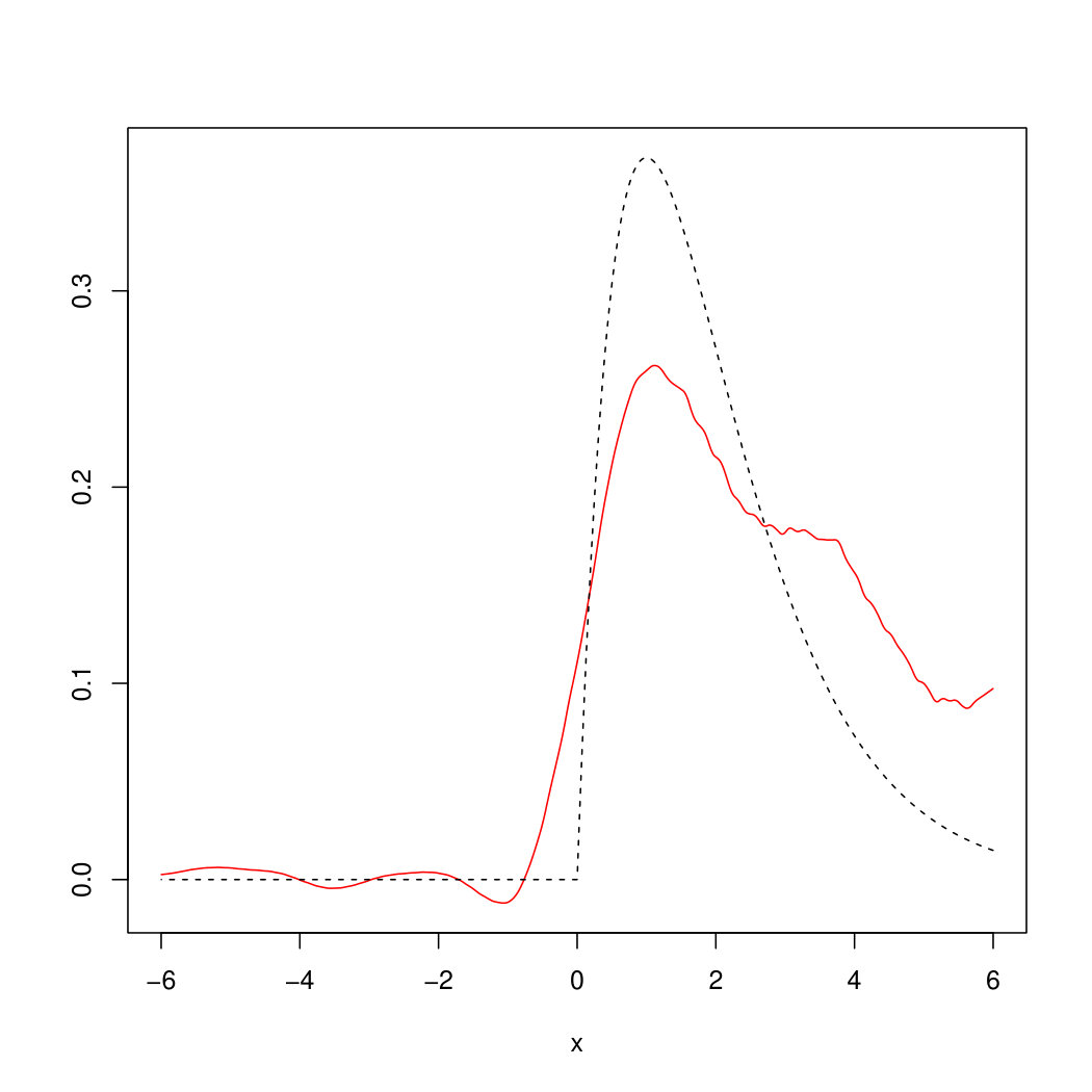 Figure 5
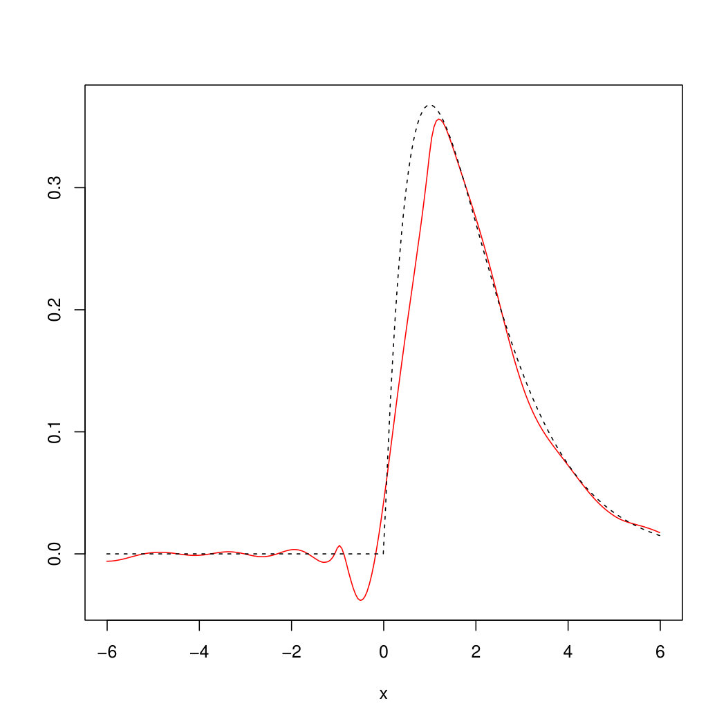 Figure 6
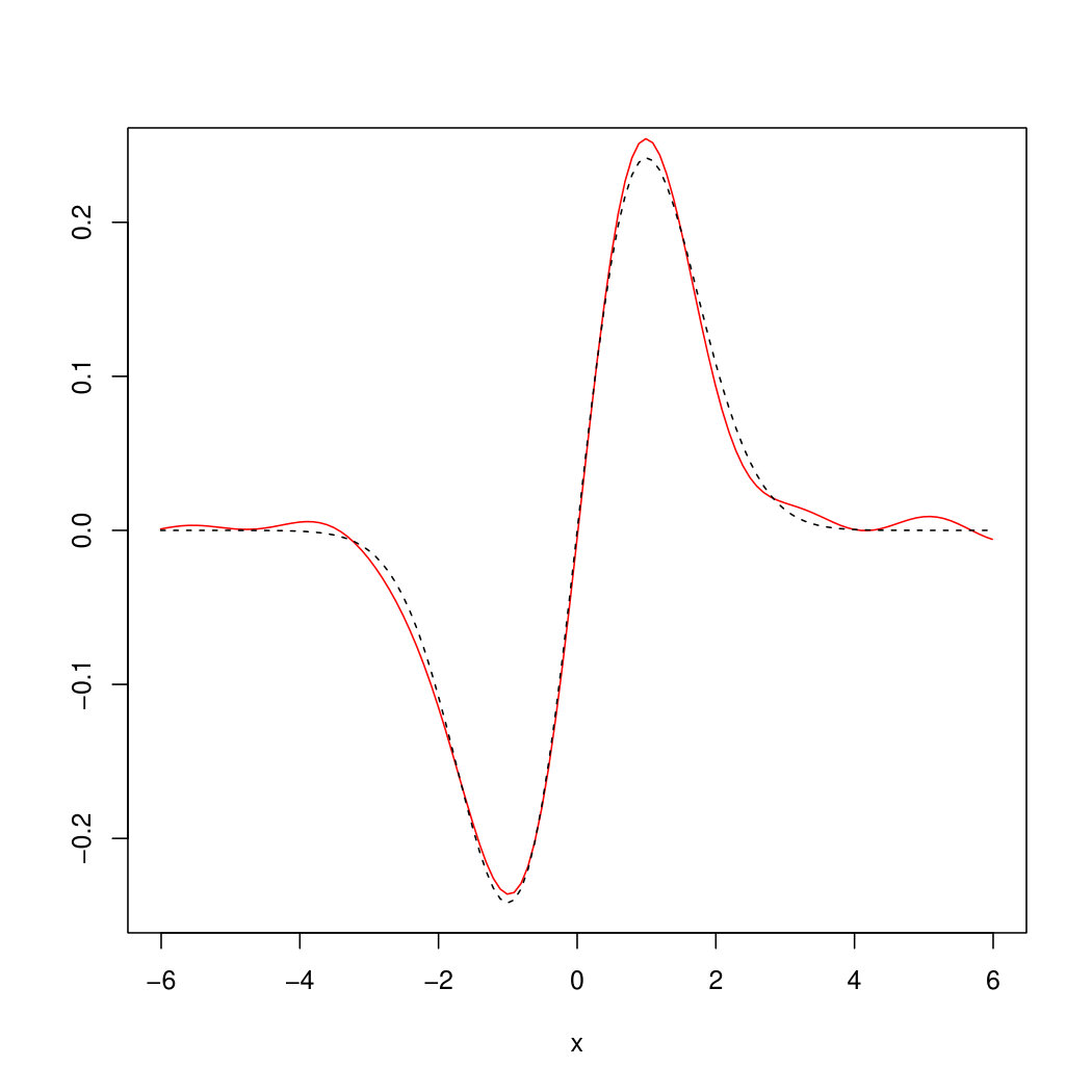 Figure 7
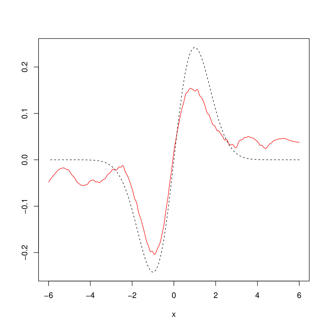 Figure 8
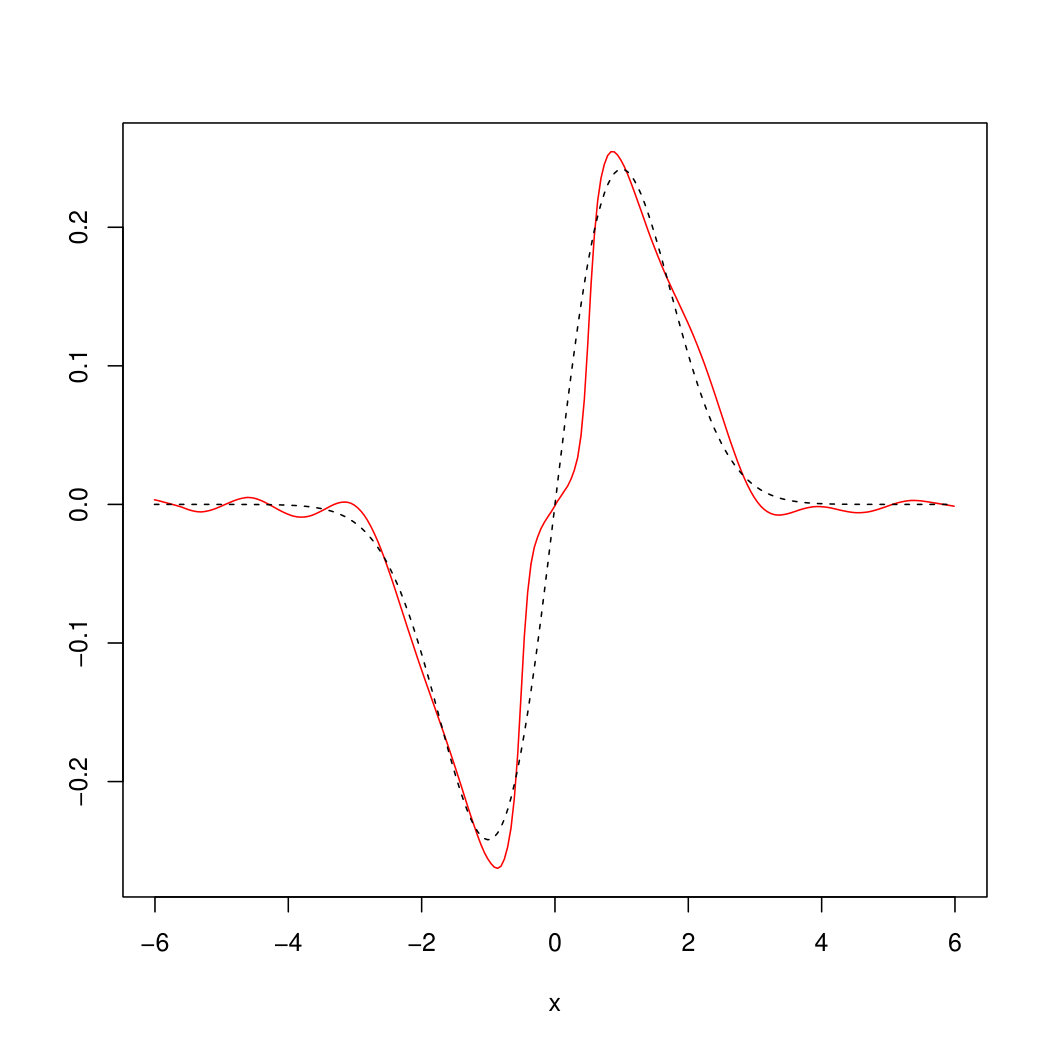 Figure 9
| Method of estimation | ||||
|---|---|---|---|---|
| plug-in | Fourier | OnB | ||
| mean | 0.005291606 | 0.0005609035 | 0.02257974 | |
| sd | 0.0004369446 | 0.0003471337 | 0.001865197 | |
| mean | 0.1240124 | 0.1306668 | 0.1446655 | |
| sd | 0.004051844 | 0.005115684 | 0.007453711 | |
| Method of estimation | ||||
|---|---|---|---|---|
| plug-in | Fourier | OnB | ||
| mean | 1031.18 | 74.95 | 2726.07 | |
| sd | 54.19 | 3.66 | 1120.59 | |
| mean | 1262.24 | 121.24 | 3165.08 | |
| sd | 13.93 | 18.14 | 721.25 | |
Peer Reviews
No public reviews on file for this paper yet. If you reviewed it on a platform where reviews are public (OpenReview, ICLR, NeurIPS, ICML), you can paste yours below so the community can read it here.
Videos
No videos yet. Explain this paper in a talk, walkthrough, or lecture? Add one.
An Inverse Problem for Infinitely Divisible Moving Average Random Fields
W. Karcher, S. Roth, E. Spodarev, C. Walk
Abstract
Given a low frequency sample of an infinitely divisible moving average random field with a known simple function , we study the problem of nonparametric estimation of the Lévy characteristics of the independently scattered random measure . We provide three methods, a simple plug-in approach, a method based on Fourier transforms and an approach involving decompositions with respect to -orthonormal bases, which allow to estimate the Lévy density of . For these methods, the bounds for the -error are given. Their numerical performance is compared in a simulation study.
Ulm University
Keywords: Infinitely divisible random measure; stationary random field; Lévy process, moving average; Lévy density; Fourier transform; Banach fixed–point theorem.
1 Introduction
Let be a stationary infinitely divisible independently scattered random measure with Lévy characteristics , where , and is a Lévy density. Let furthermore be a moving average infinitely divisible random field on defined by
[TABLE]
with Lévy characteristics , where is a simple function. Suppose a sample from is available. The problem studied in this paper is the nonparametric estimation of . For any simple function with congruent sets , in (1) has the same distribution as a linear combination of i.i.d. infinitely divisible random variables. Therefore, existence and uniqueness of a characteristic triplet with the property that a certain linear combination of independent random variables with the corresponding infinitely divisible distribution leading to a random variable with Lévy characteristics becomes a characterization problem for such distributions. For certain distributions, namely the Poisson and the Gaussian one as well as a mixture of both, all possible distributions for the summands in the linear combination can be described (see e.g. [1]). The disadvantage of those characterization theorems is that they do not give any information about the involved parameters (expectation and variance of each summand) and so it is not possible to derive sufficient conditions for the existence of a solution in terms of the kernel function . Therefore, to solve the inverse problem, we prefer to use concrete relations between the characteristic triplets of and (Section 3) given in terms of .
The recent preprint [2] covers the case estimating the Lévy density of the integrator Lévy process of a moving average process . It is assumed that . The estimate is based on the inversion of the Mellin transform of the second derivative of the cumulant of . A uniform error bound as well as the consistency of the estimate are given. It is not assumed that is simple, however, main results are subject to a number of quite restricting integrability assumptions onto and as well as mixing properties of that are tricky to check. Additionally, the logarithmic convergence rate shown there (cf. [2, Corollary 1]) is too slow.
In our approach, we develop the ideas of [3] and use Banach fixed–point theorem combined with a recursive iteration procedure (Theorem 4.1) to give sufficient conditions for the existence of a (unique) solution of our (generally speaking, ill–posed) inverse problem . We consider simple functions since
in applications, is mainly discretely sampled, 2. 2.
any can be approximated in the –norm by a sequence of simple (attaining a finite number of values) arbitrarily well, 3. 3.
this allows us to use relatively simple arguments in the proofs and to avoid complex assumptions that are not easy to verify, 4. 4.
the –convergence rate of our estimates of to its true value is , cf. Corollaries 5.2 and 5.3.
The case of arbitrary integrable is considered in our forthcoming paper [4].
This paper is organized as follows: Section 2 gives an introduction to the theory of infinitely divisible random measures and stochastic integrals as well as a short overview on -dependent and -mixing random fields together with some moment inequalities (cf. Section 2.3). In Section 3, we describe the inverse problem in detail and give formulas for the relationship between the characteristics and . In Section 4, we obtain sufficient conditions for the existence and uniqueness of the solution of the direct problem, i.e. we propose conditions under which the mapping is a bijection. It turns out that this holds true if either one of the coefficients dominates all the others or one of them repeats often enough in some sense.
Estimates for the characteristic Lévy triplet of are given in Section 5 for pure jump infinitely divisible random fields. Here we use the ideas of [5], [6] and [7] originally designed to estimate the Lévy density of Lévy processes. The main result of this section is the proof of the upper bound for the -error of the proposed estimator without the assumption of independence of observations . The estimation error remains of the same structure as in the Lévy process case if the random field is assumed to be -dependent or -mixing. For the ease of reading, long proofs of the results of this section are moved to Appendix. Section 6 provides three estimation approaches for the density of . The first method is a simple plug-in approach. The second one, the Fourier method, is based on the idea of estimating first the Fourier transform of followed by another plug-in procedure. The last method uses orthonormal bases in the Hilbert space , , for a representation of the solution of the inverse problem. After approximating by cutting off its expansion, the coefficients can be estimated by solving a system of linear equations. For all our methods, we propose upper bounds for the -estimation error. In the last section, the performance of the methods is compared by numerical simulations.
2 Preliminaries
Introduce some notation that will be used throughout this paper.
By we denote the Borel -field on the d-dimensional Euclidean space . The Lebesgue measure on is denoted by . We briefly write if we integrate w.r.t. on . The collection of all bounded Borel sets in will be denoted by . For any measurable space we denote by , , the space of all -mesurable functions with . Equipped with the norm , becomes a Banach space and even in the case a Hilbert space with scalar product , for any . With (i.e. if ) we denote the space of all real valued bounded functions on . In case we denote by
[TABLE]
the Sobolev space of order equipped with the Sobolev norm , where is the Fourier transform on . For , is defined by , . If or , , with being the counting measure, then we write as usual instead of and all integrals above become sums. Throughout the rest of this paper denotes a probability space. Note that in this case is the space of all random variables with finite -th moment as well as , if and if , for any . For an arbitrary set we introduce furthermore the notation for its cardinality. Let be the support set of a function . Denote by the diameter of a bounded set .
2.1 ID Random Measures and Fields
Recall some definitions and give a brief overview of infinitely divisible (ID) random measures and fields.
Let be an ID random measure on some probability space , i.e. a random measure such that
for each sequence of disjoint sets in it holds
- (a)
a.s., whenever , 2. (b)
is a sequence of independent random variables. 2. 2.
the random variable has an ID distribution for any choice of .
Due to the infinite divisibility of the random variable , its characteristic function, which will be denoted by , has a Lévy-Khintchin representation which will assumed to be of the form
[TABLE]
with
[TABLE]
where , and is a Lévy density, i.e. . The triplet will be referred to as Lévy characteristic of . It uniquely determines the distribution of the process . A general form for the characteristic function of any ID random measure can be found in [8, p. 456]. The particular structure of the characteristic function in (2) means that the random measure is stationary with control measure given by
[TABLE]
Now we can define the stochastic integral w.r.t. the ID random measure .
Let be a real simple function on , where are pairwise disjoint. Then for every we define
[TABLE] 2. 2.
A measurable function is said to be -integrable, if there exists a sequence of simple functions as in
-
such that
-
(a)
, -a.e. 2. (b)
for every , the sequence converges in probability as . In this case we set
[TABLE]
A useful characterization of -integrability is given in [8, Theorem 2.7]. Now let be a family of -integrable functions induced by the Borel measurable map . Then we define the ID moving average random field by
[TABLE]
A random field is called ID if its finite dimensional distributions are ID. The random field defined in (4) is stationary and ID and the characteristic function of of is given by
[TABLE]
with given in (3). It is easy to see that
[TABLE]
with
[TABLE]
where , , is the Lévy density of , denotes the support of and the function is defined via
[TABLE]
The triplet is again referred to as Lévy characteristic (of ) and determines the distribution of uniquely. Note that due to -integrability of all integrals above are finite. This immediately implies that .
For details on the theory of infinitely divisible measures and fields with spectral representation as well as proofs for the above stated facts we refer the interested reader to [8].
2.2 -Dependent and -Mixing Random Fields
A random field , defined on is called -dependent if for some and any finite subsets and of the random vectors and are independent, whenever
[TABLE]
for all and . Note that a random field as in (4) is -dependent, if the support of is bounded with .
Besides, we define the notion of -mixing random fields. The mixing coefficient is defined as follows. For any , let be the –field generated by random variables . Let furthermore and be two sub--fields of . Define
[TABLE]
and for
[TABLE]
where for . A random field on is called -mixing or uniform mixing if
[TABLE]
for any . Equation (11) is called -mixing condition, see e.g. [9] for more details on mixing.
2.3 Moment and Exponential Inequalities for Random Fields
In the literature, one can find many moment and exponential inequalities for sums of independent and identically distributed random variables, e.g., the classical* Rosenthal inequality* [10] or the Bernstein inequality [11].
Similar inequalities hold true for random fields. For define the set , where denotes the lexicographic order. Let for . For set for
[TABLE]
Figure 1 shows the sets and for some . The following two results can be found in [12, pp. 12-14].
Theorem 2.1**.**
Let be a centered and square-integrable random field. Let be a finite subset. Then for any it holds
[TABLE]
where , for and for any .
Theorem 2.2**.**
Let be a field of bounded and centered random variables. Set . Then for any positive and real it holds
[TABLE]
Note that Theorem 2.1 and Theorem 2.2 are extensions of Burkholder’s [13] and Azuma’s [14] inequality for martingales. The next theorem [9, p. 32] states a Rosenthal-type inequality for -mixing random fields.
Theorem 2.3**.**
Let be a random field. For let be the smallest even integer such that . Assume
[TABLE]
for all with , . Let be a finite subset of . If belongs to and is centered for all , then there exists a positive constant that depends on and on the mixing coefficient of such that
[TABLE]
Additionally, the following result can be found in [12, p. 15].
Theorem 2.4**.**
Let be a strictly stationary field of bounded and centered random variables. Take and set
[TABLE]
For any , set for . For any positive real we have
[TABLE]
3 Inverse Problem
In this section, we give a description of the inverse problem treated in this paper.
Let be a homogeneous ID random measure with Lévy characteristics . Consider to be a simple function, where and pairwise disjoint, . Assume furthermore to be an ID moving average random field of the form
[TABLE]
where for an arbitrary set .
The Inverse Problem**.**
Given observations at points of the random field , estimate the Lévy triplet of the ID random measure .
Formulas (6) and (7) then become
[TABLE]
with defined in (8). For known , the above equations are easily solvable w.r.t. and , thus providing an estimation approach for and . So, given , the main point is now to find a solution of the last equation. In the next section, we give some sufficient conditions under which a solution exists and is unique.
4 Existence and Uniqueness of a Solution for
In the following, we assume w.l.o.g. that for all . Typically it is common to estimate rather than itself, since many of the estimators for Lévy densities are based on derivatives of the Fourier transform (in the context of Lévy processes, see e.g. [5, 6, 7]). For this purpose let be a measurable function such that
[TABLE]
[TABLE]
A sufficient condition for (16) to hold is
[TABLE]
Indeed, the Cauchy-Schwarz inequality yields
[TABLE]
Examples of functions satisfying (16)–(18) are , , and , . Consider the modified equation
[TABLE]
It is understood in -sense, where it is assumed that and are both in . Let be the set of all indices of coefficients that coincide with . Denote by its cardinality. Define
[TABLE]
The following theorem states conditions, under which equation (19) has a unique solution for fixed .
Theorem 4.1**.**
Let a function be given as above. Then equation (19) has a unique solution for any if
[TABLE]
The solution is given by the formula
[TABLE]
Proof.
Let . Define the operator by
[TABLE]
Then formula (19) yields a fixed point of , i.e., is a solution of equation
[TABLE]
It is straight forward to see that for any functions it holds
[TABLE]
i.e. is a contraction. By Banach fixed-point theorem there exists a unique solution to the equation (23) which shows the first part of the theorem. Relation (22) can easily be obtained by iterating equation (23) w.r.t. . ∎
Remark 4.2**.**
Note that the choice of in this setting is arbitrary. The statement of Theorem 4.1 does not depend on a certain order of the coefficients . In particular, this means that in the definitions of and can be replaced by any other coefficient , . Consequently, substituting by in Theorem 4.1 leads to the same solution . Indeed, let , be any other coefficient that fulfills the conditions of Theorem 4.1, and let be the corresponding solution of (19). Then
[TABLE]
Due to Theorem 4.1, this equation has a unique solution. Since [math] is a solution it thus follows that (in -sense).
Remark 4.3**.**
Theorem 4.1 gives sufficient conditions for the existence and uniqueness of a solution (22) of equation (19). If condition (21) fails to hold, no solution as well as infinitely many solutions of (19) are possible. One can easily construct corresponding examples illustrating that. Consider e.g. , and . Now choose to be any odd function satisfying (16)-(18). Clearly condition (21) is not fulfilled. Then (19) becomes
[TABLE]
Let be any even function, a.e. Then (24) has no solution since its right–hand side is odd. 2. 2.
If, on the other hand, a.e. then any even -function is a solution of (24).
Note that condition (17) ensures that for any . This condition is necessary. Consider e.g. , , , as well as , . Then, except for (17), all conditions of Theorem 4.1 are fulfilled, but in this case. Thus (22) cannot be an -solution.
Remark 4.4**.**
Condition (21) is not necessary for the existence and uniqueness of a solution of equation (19). As a counterexample, consider , , , , and . If
[TABLE]
then none of the coefficients fulfills (21). In our paper [4] we prove necessary and sufficient conditions for existence and uniqueness of a solution of integral equation (7). It can be shown that satisfies those conditions and hence there is a unique solution of (19) for any .
Condition (21) means that one of the coefficients (here ) dominates all others either in its magnitude or in its frequency . To illustrate this, consider any power function with and . Then , and the equation is solvable w.r.t. if
[TABLE]
In particular, if this means that . If is strictly positive and super-homogeneous of degree , i.e.
[TABLE]
for all and some , then condition (17) is fulfilled if all the coefficients have the same sign. Then (21) holds if
[TABLE]
5 Estimation of for Pure Jump ID Random Fields
Modern statistical literature contains quite a number of methods to estimate the Lévy density of if , i.e., is a Lévy process, see [15, 7, 5, 16, 6, 17, 18], [19] and references therein. They range from moment fitting and maximum likelihood ratio to inverse Fourier methods based on the empirical characterstic function of . For simplicity, one often assumes that the drift and the Gaussian part of vanish, thus letting be a pure jump Lévy process.
In the recent preprint [19], the problem of estimation of the Lévy measure of was solved for compound Poisson Lévy processes using variational analysis on the cone of measures and the steepest descent method of minimizing of a certain risk functional implemented for the discrete (atomic) measures. The resulting estimate of can be obtained out of these measures by smoothing.
For all our estimation approaches in the next section, either estimators for or at least for its Fourier transform are required to proceed with the estimation of . Therefore we adopted an estimation procedure from [16, 5] for pure jump Lévy processes to estimate . The main difference to Lévy processes is in our case the assumption of independent increments which obviously is not given for random fields in arbitrary dimension . Nevertheless, assuming to be -dependent or -mixing allows us to use the same ideas for the estimation of .
Consider a stationary random field as in (14) with characteristic function given by
[TABLE]
Note that its logarithm coincides with formula (5) by taking and . Under the additional assumption it holds
[TABLE]
that is equivalent to
[TABLE]
where (taking ) and denotes the Fourier transform of . Now let be discretely observed on a regular grid with mesh size , i.e. we consider the random field where
[TABLE]
For a finite nonempty set with cardinality let be a sample from . By taking the empirical counterparts
[TABLE]
of and on the right–hand side of (25) an estimator for can be defined as
[TABLE]
where
[TABLE]
The indicator function on the right hand side of (29) ensures the stability of the estimator for small values of . Based on this idea Comte and Genon-Catalot [16] provided the estimator
[TABLE]
for . We make the following assumptions: for a
(H1)
(H3)
and such that for all
[TABLE]
(H4)
where is as in (H3).
Assumptions (H1)– are moment conditions for . Assumptions (H3)– (H4) are used to compute –error bounds and rates of convergence of Lévy density estimates, cf. [5]. For the random field we define
[TABLE]
where , . Under condition , it holds and hence \operatorname{\mathbb{E}}\big{(}\xi_{t}^{(i)}(u)\big{)}^{2}<\infty, \operatorname{\mathbb{E}}\big{(}\tilde{\xi}_{t}^{(i)}(u)\big{)}^{2}<\infty for , and . Introduce the notation for any random function s.t. .
The following -error bounds for will be proven in Appendix.
Theorem 5.1**.**
Assume that (H1), hold and that we observe the strictly stationary random field . Further assume that either
- (i)
the field is -dependent or
- (ii)
the random field is -mixing such that equations (12)–(13) hold.
Then for all
[TABLE]
where is a constant, is given by for , and is the sample size.
Notice that random fields (14) are –dependent with since a simple function has a compact support. Introduce the notation .
The following corollary is an immediate consequence of Theorem 5.1.
Corollary 5.2**.**
If additionally (H3) and (H4) hold then the bound in Theorem 5.1 can be improved to
[TABLE]
where is constant.
Corollary 5.3**.**
Under the assumptions of Corollary 5.2 it holds
[TABLE]
where .
The upper bound (31) allows to choose the cut–off parameter optimally by minimizing the right–hand side expression in (31) numerically. Choosing such that yields the –consistency of the estimate .
6 Estimation of the Lévy Density
In the following Section three different estimation approaches will be discussed. The plug-in and the Fourier method are both based on formula (22), whereas the third one, which uses orthonormal bases (OnB’s) in , is totally different from them. For this reason, the problem will be reformulated in terms of –OnB’s there. Nevertheless it turns out that the sufficient conditions for the existence of a solution do not change essentially.
6.1 Plug-In Estimator
Let be an estimator for . We now consider a simple plug-in estimator of defined by
[TABLE]
where denotes the sample size and is a certain cut-off parameter depending on . The following theorem gives a bound for the mean square error .
Theorem 6.1**.**
Consider and let be an estimator of . Let furthermore the conditions of Theorem 4.1 be fulfilled. Then with the notation given there it holds
[TABLE]
In particular, if is an -consistent estimator for (i.e., as ) then is as well an -consistent estimator for .
Proof.
First of all, we observe that for each and it holds
[TABLE]
By relation (19) and condition (17), as well, cf. Lemma 6.2. Using formula (22) it follows by triangle inequality and a simple integral substitution that
[TABLE]
Since the consistency result follows immediately from this approximation. ∎
Lemma 6.2**.**
Let , , and condition (17) hold. Then .
Proof.
Using relation (19), condition (17) and triangle inequality, we get
[TABLE]
∎
Using the estimator in practice reveals that
the choice suffcies completely to get good results due to fast convergence of the geometric series in (33), 2. 2.
oscillates much in a neighborhood of the origin.
Hence, one has to regularize it applying a usual smoothing procedure. Convolve with a smoothing kernel which depends on its bandwidth and satisfies the following assumptions:
(K1)
, for all
(K2)
where is a constant independent of
(K3)
for all , where is a constant.
For the resulting estimator
[TABLE]
we give an upper bound of its mean square error and prove its consistency as and .
Theorem 6.3**.**
Let for some , and let be an estimator of . For a kernel satisfying assumptions * (K1) –(K3), it holds*
[TABLE]
where
[TABLE]
Proof.
By triangle inequality, Plancherel identity and convolution property of we have
[TABLE]
since by relation (32). By assumption (K3) and Cauchy-Schwartz inequality, we have
[TABLE]
The rest of the proof follows by observing that for
[TABLE]
as . ∎
There are many examples of kernels satisfying assumptions (K1)–(K3), e.g., the Gaussian kernel . Since , (K1)–(K2) are trivial. Condition (K3) holds from the inequality
[TABLE]
Another class of examples is provided by , , where is a nonnegative function such that , and is a Lipschitz continuous function. While (K1)–(K2) trivially hold in this case, (K3) can be seen from the following lemma.
Lemma 6.4**.**
Let be as above. Then
[TABLE]
where with being the Lipschitz constant of .
Proof.
Because of and the Lipschitz continuity of it follows
[TABLE]
Thus . ∎
Corollary 6.5**.**
Choose , as in Section 5. Under the assumptions of Theorem 4.1, Corollary 5.2 and Theorem 6.3 the estimator is -consistent for as and .
Proof.
Applying Theorem 6.1 and Corollary 5.3 yields as for any sequence . Relation as finishes the proof. ∎
Remark 6.6**.**
The choice of bandwidth in (34) can be made by solving the following minimization problem numerically:
[TABLE]
which means that we are seeking for a sufficiently smooth estimate . Assuming that is a –smooth function of parameter and that the differentiation with respect to and the integral can be interchanged we get by Plancherel identity and convolution property of that
[TABLE]
For easy particular functions the Fourier transform of can be usually calculated explicitly. In contrast, has to be estimated from the data, compare Section 6.2 for . There, we use the estimate to assess .
6.2 Fourier Approach
A common strategy in the estimation of (e.g. in the case of Lévy processes) is first to estimate its Fourier transform and then to invert it. This causes an error in the estimation of the Fourier transform and additionally in the inversion procedure. Using plug-in estimators of Section 6.1, this may increase the estimation error for . For this reason, here we estimate directly to recover .
From now on, set for some . In other words, equation (22) is of the form
[TABLE]
where and . Suppose that and the conditions of Theorem 4.1 are fulfilled. Then as well by Lemma 6.2.
The following construction of and is motivated by estimation approaches for the characteristic triplet of Lévy processes (see e.g. [7]). Taking Fourier transforms on both sides of (37) yields
[TABLE]
for . Let be any estimator for the Fourier transform of . Then we define the estimator for via
[TABLE]
. If is locally square integrable, an estimator of is constructed for some as
[TABLE]
The last expression can be rewritten as
[TABLE]
with being an estimator of .
Remark 6.7**.**
The estimator (28) from Section 5 is locally square integrable. In this case an appropriate choice for the parameter can be achieved e.g. by minimizing the right-hand side of (31) for any fixed sample size (see also the discussion following Corollary 5.3).
Similar as in Theorem 6.1 one can obtain an upper bound for the -error. With the notation we get
[TABLE]
where , . Assume
[TABLE]
Choose the estimator of in an –consistent way. Then, as in an appropriate manner, the above upper bound (39) tends to zero, and is –consistent for . For instance, one can choose from Section 5, which is –consistent under assumptions of Corollary 5.2.
Assume, in addition to (40), that By (31), the upper bound of is monotonously non–decreasing in . Since
[TABLE]
[TABLE]
as such that .
6.3 Orthonormal Basis Approach
Since the series representation (22) is sensitive to noise and bad estimates for , the aim is to obtain an estimation approach that uses (local) orthonormal bases (e.g., Haar wavelets) of . Moreover, from the numerical point of view it is much more convenient to find a solution only on a finite interval. For this reason, the problem of Section 4 should be reformulated for functions on with support contained in a finite interval. For , consider
[TABLE]
to be the closed linear subspace of equipped with the usual scalar product on . Find a function that fulfills equation (19) for fixed . Because of the scalings on the right hand side of this equation, we have to extend the assumptions on and the coefficients a bit. Let be the largest coefficient and define . Then for it follows that . Since is the largest coefficient, it holds moreover that , for all , i.e. for all . For this reason the restriciton of the function from the proof of Theorem 4.1 is a map on . Then one can show the following theorem with the same arguments applied to .
Theorem 6.8**.**
Let , be as in Theorem 4.1, and let with defined as before. Assume furthermore that and relation (21) holds. Then there exists a unique function such that
[TABLE]
a.e. on . The solution can be expressed as in (22).
Note that the solution fulfills the equation a.e. on the whole interval , whereas (41) holds only on , which is merely the same if , i.e. in the case . Notice that means that the random field has a compound Poisson marginal distribution if .
The last theorem stated the existence of a solution of the fixpoint equation or equivalently for
[TABLE]
Now let be an orthonormal basis (OnB) of . Since it holds
[TABLE]
Note that because of the function is in for all . Set
[TABLE]
Then we can conclude that there exists a solution of (42) if and only if the function admits a representation with some -sequence . In this case, a solution is given by . It is unique if and only if the scalar sequence is unique. In other words, the problem is characterized by the operator ,
[TABLE]
If is surjective there exists a solution. If it is bijective the solution is unique. It is clear now that under the conditions of Theorem 6.8 the operator is a bijection. Nevertheless, let us reformulate this theorem in terms of the OnB and give another proof for it.
Theorem 6.9**.**
Let be an OnB of , and let the conditions of Theorem 6.8 be fulfilled. Then there exists a unique sequence such that the operator is one–to–one.
Proof.
We would like to show that the system is a basis for . First we show, by contradiction, that
[TABLE]
Therefore assume that . Since is a closed subspace of it follows by Riesz lemma (see e.g. [20]) that for any there exists a function with such that , for all . Now choose Then we can write . Define the sequence via , . Since it follows . Clearly, we have . By triangle inequality, a substitution in the integral and the definition of it can be observed that
[TABLE]
which is a contradiction to the fact that , i.e. .
In the second step of the proof, we use [21, Theorem 3.1.4] to show that is a basis for . Therefore we have to verify the assumptions there. First of all, we observe that are non-zero functions, since
[TABLE]
where the latter is strictly positive, i.e. is a sequence of non-zero functions in the Hilbert space . Now let be an arbitrary real valued sequence and with . Show that there exists a constant such that . If then this relation is obviously true for any choice of . Otherwise,
[TABLE]
Thus, we have
[TABLE]
This means is a basis for , i.e. for any function there is a unique scalar sequence with . Since
[TABLE]
the sequence is furthermore an element of . Choosing
[TABLE]
completes the proof. ∎
Note that the proof of the last theorem shows that the system is a basis for the -subspace . Therefore we can orthonormalize it by Gram–Schmidt method to an OnB of given by and succesively
[TABLE]
Now let be any estimator for and let be the orthogonal projection of onto the -dimensional subspace which is given by . Define the sequence by
[TABLE]
Then the orthogonal projection of onto is
[TABLE]
Now, an estimator for will be constructed as follows:
- 1.)
Let be the unique solution to
[TABLE]
Set
[TABLE] 2. 2.)
Then we define
[TABLE]
Equation (44) comes from the fact that for any , if and only if . Note that whenever since is a linear combination of . In particular, formula (44) stays true if . Due to that, the system of linear equations there becomes diagonal and can easily be solved by backward substitution.
Theorem 6.10**.**
Let and be an estimator of . Let furthermore be the orthogonal projection of onto . Then under the conditions of Theorem 6.9 it holds for as in (45) that
[TABLE]
where , .
Proof.
First of all, it holds
[TABLE]
and therefore
[TABLE]
with defined by , , compare (43). Then
[TABLE]
By (6.3) together with the triangle inequality we get
[TABLE]
Taking into account that \left\|\sum\limits_{i=m+1}^{\infty}x_{i}\eta_{i}\right\|_{2}\geq\frac{n_{1}}{|f_{1}|}\big{(}1-e(f,h)\big{)}\left\|\sum\limits_{j=m+1}^{\infty}x_{j}\psi_{j}\right\|_{2} the statement of the theorem follows by (48). ∎
Remark 6.11**.**
The term in (46) is the approximation error of by the first summands of its series. As , the upper bound (46) tends to \frac{|f_{1}|}{n_{1}\big{(}1-e(f,h)\big{)}}\|\bar{g}_{1}-\hat{\bar{g}}_{1}\|_{\cdot}. In order to estimate , the method of Section 5 can be used if the random field satisfies the assumptions given there. In this case, Corollaries 5.2 and 5.3 yield an upper bound for leading to –consistent estimates of .
Since the estimator in (45) is strongly oscillating, a smoothed version of is considered here, where is a smoothing kernel with properties (K1)-(K3) from Section 6.1. It is clear that , , because both are in by assumption. If additionally for some then it immediately follows from the proof of Theorem 6.3 that
[TABLE]
with given in (36). The bandwidth can be chosen as in Remark 6.6.
7 Numerical Performance of the Estimators
In order to compare the three approaches of Section 6, we consider to be a compound Poisson random variable
[TABLE]
where is a sequence of independent and identically distributed random variables, independent of . Then for any simple function with for all it holds
[TABLE]
where are i.i.d. with .
In the following examples, we assumed , , , , as well as . Then is the density of the random variable , and due to formula (15), is given by
[TABLE]
or, equivalently,
[TABLE]
where and , . Note that the coefficients fulfill conditions of Theorem 4.1, i.e. for given there exists a solution to the above equation. In our examples, we simulated the random field on an integer grid. The estimators for based on the corresponding sample with sample size were compared to the original for the following examples:
[TABLE]
For the estimators based on the Fourier method from Section 6.2, the parameter is chosen due to Corollary 5.3, cf. Section 5. For both the plug-in (Section 6.1) and the Fourier method, we used furthermore the cut-off parameter . For the smoothing procedure, the Epanechnikov kernel
[TABLE]
with bandwidths and was used in examples (49) and (50) respectively, chosen according to Remark 6.6. For the OnB method, Haar wavelets on for were used together with the cut–off parameter . The parameter and the bandwidth for the estimator in (45) (using Epanechnikov kernel ) were chosen based on a simulation study with different parameters. It turned out that visually the best choice for the example in (49) is , whereas for the example in (50) the parameters , turned out to be optimal. Figures 2 and 3 show realizations of the estimated (red) by our methods compared to the original (dashed) from examples (49) and (50).
The empirical mean and the standard deviation of the mean square errors of our estimation (assessed upon estimation results for out of simulations of ) are given in Table 1. It is seen there that plug-in and Fourier methods perform equally well whereas the mean error for the OnB method is significantly higher. Regarding their computation times (see Table 2), the Fourier approach outperforms the others since its algorithm is at least times faster. To summarize, we recommend the Fourier method for the estimation of unless the plug-in approach can be used under milder assumptions on and . This essentially depends on the estimator for which is chosen as a plug-in.
Appendix
Here we give a proof of Theorem 5.1 and its corollaries. Before doing so we prove auxiliary statements.
Lemma 7.1**.**
Let be a random field defined in (26) satisfying such that is either
- (i)
-dependent or
- (ii)
-mixing and condition (12) holds.
Furthermore, let be a finite subset, , and let and . Then
[TABLE]
where is a constant.
Proof.
It holds that
[TABLE]
- (i)
By Theorem 2.1 it holds for , and
[TABLE]
To determine expression it is useful to decompose it into two parts. The first part consists of all for which and the second part contains all other . Hence,
[TABLE]
For the first part it holds due to –dependence of that
[TABLE]
since is centered. Furthermore, for the second sum in expression it follows by Hölder inequality that
[TABLE]
Let and . This set is shown in Figure 4 for .
Note that for due to stationarity of
[TABLE]
Therefore, for all and it holds that \bigl{\|}\xi^{(i)}_{t}(u)\bigr{\|}_{2}\leq 2\|Y_{0}\|_{2}. Applying this to ((i)), we get \bigl{\|}\xi^{(i)}_{t}(u)\bigr{\|}_{2}\sum_{k\in\tilde{V}_{t}^{1}}\bigl{\|}\xi^{(i)}_{k}(u)\bigr{\|}_{2}\leq 4n_{t}\|Y_{0}\|_{2}^{2}. Moreover, it follows
[TABLE]
with . By Ljapunov inequality, it holds
[TABLE]
- (ii)
Using Theorem 2.3 with and applying the Ljapunov inequality we get
[TABLE]
for some constants , , where the last inequality follows by equation (52). Thus, we have
[TABLE]
where is constant.
∎
If assumption (i) holds then the constant is given by , where is the maximum over the cardinalities of the sets for every . Therefore, in the first case the constant depends on . In the second case the constant depends on the mixing coefficient by Theorem 2.3.
Lemma 7.2**.**
Let and where . Under the assumptions of Lemma 7.1 for there exists a constant such that
[TABLE]
Proof.
Since , is a convex function it holds
[TABLE]
- (i)
Applying Theorem 2.1 with we get for
[TABLE]
Since
[TABLE]
it follows \bigl{\|}\tilde{\xi}^{(i)}_{t}(u)\bigr{\|}_{2}^{2}\leq 4. Analogously to the calculations in the proof of Lemma 7.1 (i) we observe
[TABLE]
and hence
[TABLE]
So all in all we get from (54) that \operatorname{\mathbb{E}}\bigl{|}\hat{\psi}(u)-\psi(u)\bigr{|}^{p}\leq\frac{C_{p}}{N^{p/2}} for the constant and .
- (ii)
Using Theorem 2.3 and inequality (55) it follows for and that
[TABLE]
By equation (54) it finally follows \operatorname{\mathbb{E}}\bigl{|}\hat{\psi}(u)-\psi(u)\bigr{|}^{p}\leq\frac{C_{p}}{N^{p/2}}, where is a constant depending on and the mixing coefficient of , .
∎
The following lemma is a generalization of [22, Lemma 2.1] (proven there for independent random variables and ) to the case of weakly dependent random fields.
Lemma 7.3**.**
Under the assumptions of Lemma 7.1 together with condition (13) there exists a constant such that for
[TABLE]
Proof.
- 1.)
Let . Then it holds
[TABLE]
where the last inequality follows by Lemma 7.2 and the fact that an indicator is always smaller or equal than . In this case, we get for that
[TABLE]
- 2.)
Let . Then we get
[TABLE]
To calculate this probability, we consider assumptions (i) and (ii) separately.
- (i)
Here we can apply Theorem 2.2 and we get for
[TABLE]
where
[TABLE]
and for a random variable . By inequality (55) and -dependence
[TABLE]
Therefore, can be estimated as , with as in the proof of Lemma 7.1. For expression (57) we get
[TABLE]
- (ii)
Apply Theorem 2.4 to with for all and . Then, , and we have
[TABLE]
So we get in both cases
[TABLE]
It holds that
[TABLE]
Applying the binomial theorem and we get
[TABLE]
Therefore,
[TABLE]
So all in all, it holds
[TABLE]
that concludes the proof.
∎
Now we can finalize the proof of Theorem 5.1.
Proof of Theorem 5.1.
Note that is orthogonal to , since
[TABLE]
due to isometry property of in . By Pythagorean theorem we get
[TABLE]
and the second term can further be determined by
[TABLE]
Furthermore,
[TABLE]
First we calculate expression (I). Using the Cauchy-Schwarz inequality and applying Lemma 7.1 and Lemma 7.3 it holds
[TABLE]
where are some constants. Now we get
[TABLE]
For the second term (II) we use again Lemma 7.3. Then it holds
[TABLE]
for some . Using this, we get
[TABLE]
Part (III) can be estimated by Ljapunov inequality and Lemma 7.1 as
[TABLE]
So putting all these results together, it follows for some constant that
[TABLE]
that completes the proof. ∎
Proof of Corollary 5.2.
Consider expression (58) in the proof of Theorem 5.1. Using assumptions (H3)– (H4) there, it holds
[TABLE]
∎
Proof of Corollary 5.3.
Since is an isometry of one has
[TABLE]
by assumption (H4). Using (H3) one gets
[TABLE]
Plugging this into (30) yields the result. ∎
Acknowledgement
W. Karcher and E. Spodarev are grateful to E. V. Jensen for her hospitality during their stay at Aarhus University in February 2011 where this research was initiated. The authors thank M. Reiß for the fruitful discussions on the subject of the paper. They also acknowledge the valuable help of O. Moreva in implementing the algorithms of Section 7.
The reference list from the paper itself. Each links out to its DOI / PubMed record.
- 1[1] A.M. Kagan, Yu.V. Linnik, and R. C. Rao. Characterization Problems in Mathematical Statistics . John Wiley & Sons, New York, 1973.
- 2[2] D. Belomestny, V. Panov, and J. Woerner. Low frequency estimation of continuous–time moving average Lévy processes. ar Xiv: 1607.00896 v 1 , 2016.
- 3[3] W. Karcher. On Infinitely Divisible Random Fields with an Application in Insurance. Phd thesis, Ulm University, 2012.
- 4[4] J. Glück, S. Roth, and E. Spodarev. A solution of a linear integral equation with the application to statistics of infinitely divisible moving averages. Preprint , 2017.
- 5[5] M. H. Neumann and M. Reiß. Nonparametric estimation for Lévy processes from low-frequency observations. Bernoulli , 15(1):223–248, 2009.
- 6[6] S. Gugushvili. Nonparametric inference for discretely sampled Lévy processes. In Ann. Inst. H. Poincaré, Probab. Statist. , volume 48, pages 282–307, 2012.
- 7[7] F. Comte and V. Genon-Catalot. Nonparametric estimation for pure jump Lévy processes based on high frequency data. Stochastic Processes and their Applications , 119(12):4088–4123, 2009.
- 8[8] B. S. Rajput and J. Rosinski. Spectral representations of infinitely divisible processes. Probab. Th. Rel. Fields , (82):451–487, 1989.