On infinite divisibility of a class of two-dimensional vectors in the second Wiener chaos
Andreas Basse-O'Connor, Jan Pedersen, and Victor Rohde
TL;DR
This paper investigates the conditions under which certain two-dimensional vectors in the second Wiener chaos are infinitely divisible, providing necessary and sufficient criteria and exploring specific cases involving Gaussian squares.
Contribution
It offers new necessary and sufficient conditions for infinite divisibility of vectors in the second Wiener chaos, including detailed analysis of Gaussian square sums.
Findings
Necessary and sufficient conditions for infinite divisibility.
Easier verifiable sufficient conditions provided.
Conjecture that vectors with Gaussian square sums are infinitely divisible.
Abstract
Infinite divisibility of a class of two-dimensional vectors with components in the second Wiener chaos is studied. Necessary and sufficient conditions for infinite divisibility is presented as well as more easily verifiable sufficient conditions. The case where both components consist of a sum of two Gaussian squares is treated in more depth, and it is conjectured that such vectors are infinitely divisible.
Click any figure to enlarge with its caption.
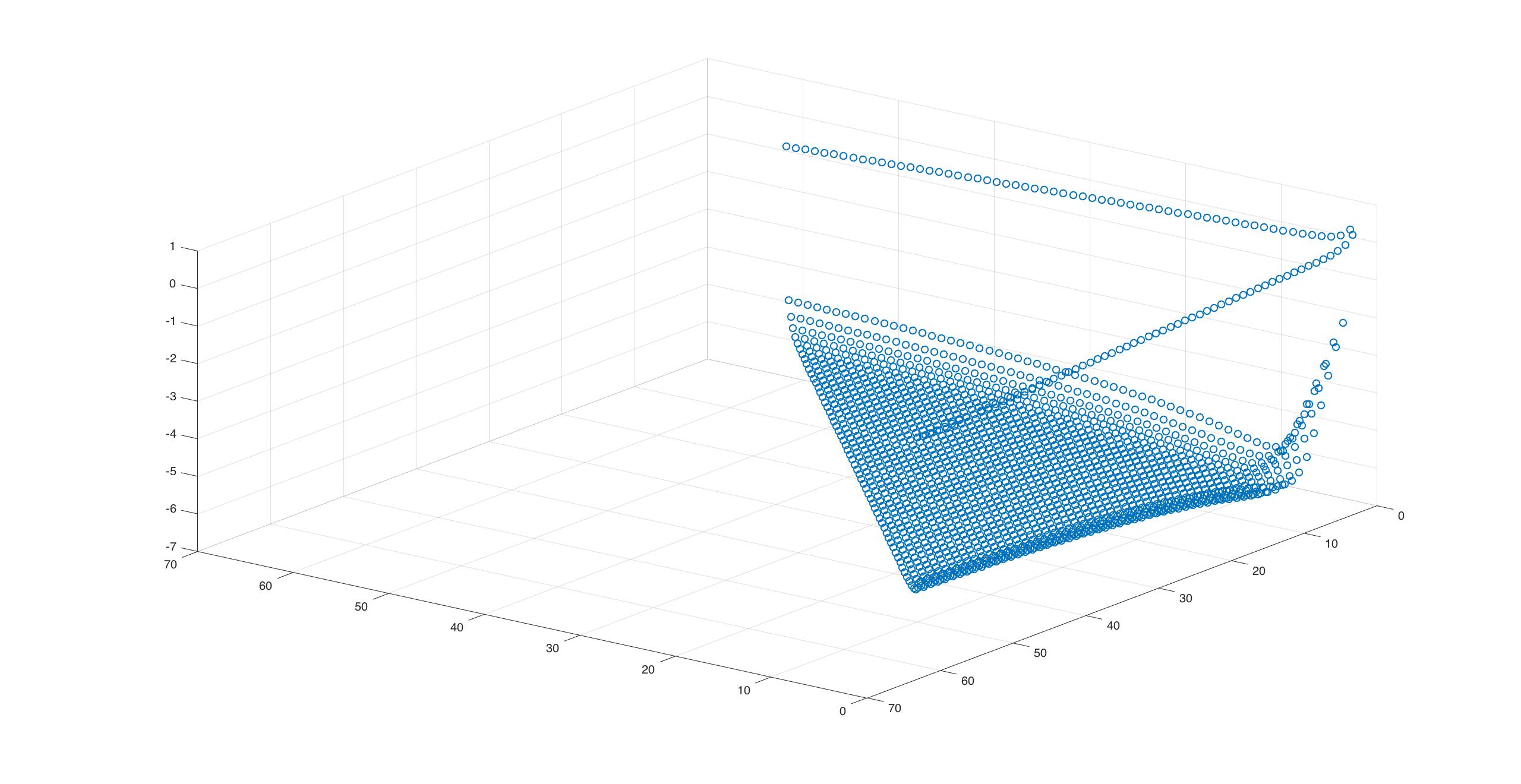 Figure 3
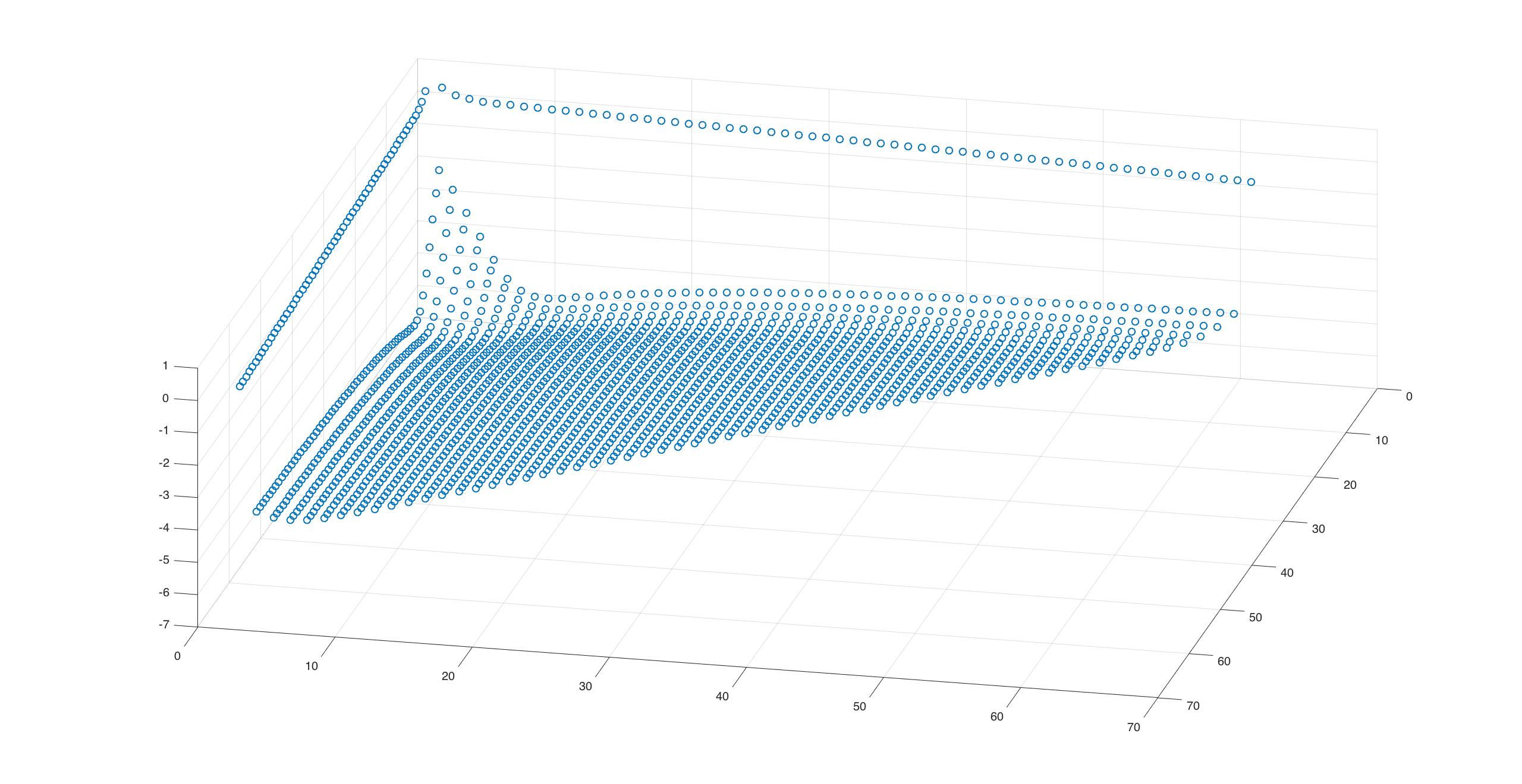 Figure 3
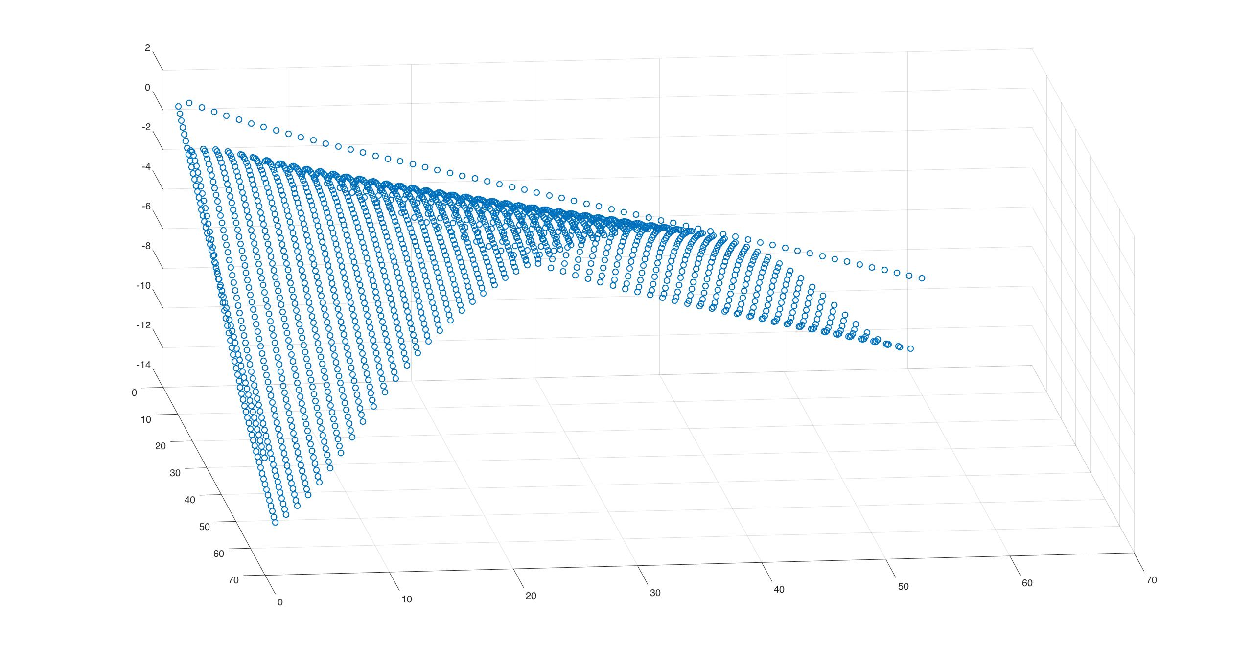 Figure 3
Peer Reviews
No public reviews on file for this paper yet. If you reviewed it on a platform where reviews are public (OpenReview, ICLR, NeurIPS, ICML), you can paste yours below so the community can read it here.
Videos
No videos yet. Explain this paper in a talk, walkthrough, or lecture? Add one.
Taxonomy
TopicsComplex Systems and Time Series Analysis · Nonlinear Dynamics and Pattern Formation · Mathematical Dynamics and Fractals
On infinite divisibility of a class of two-dimensional vectors in the second Wiener chaos
Andreas Basse-O’Connor, Jan Pedersen, Mikkel Slot Nielsen,
and Victor Rohde
Department of Mathematics
Aarhus University
{basse, jan, mikkel, victor}@math.au.dk
Andreas Basse-O’Connor, Jan Pedersen, and Victor Rohde
Abstract
Infinite divisibility of a class of two-dimensional vectors with components in the second Wiener chaos is studied. Necessary and sufficient conditions for infinite divisibility is presented as well as more easily verifiable sufficient conditions. The case where both components consist of a sum of two Gaussian squares is treated in more depth, and it is conjectured that such vectors are infinitely divisible.
Department of Mathematics, Aarhus University, E-mail adresses: [email protected] (A. Basse-O’Connor), [email protected] (J. Pedersen), [email protected] (V. Rohde)
Keywords: Sums of Gaussian squares; infinite divisibility; second Wiener chaos
MSC 2010: 60E07; 60G15; 62H05; 62H10
1 Introduction
Paul Lévy [11] raised the question of infinite divisibility of Gaussian squares, that is, for a centered Gaussian vector when can be written as a sum of independent identical distributed random vectors for any ? Several authors have studied this problem. We refer to [4, 5, 6, 7, 8, 13] and reference therein. These works include several novel approaches and gives a great understanding of when Gaussian squares are infinitely divisible. In this paper we will provide a characterization of infinite divisibility of sums of Gaussian squares which to the best of our knowledge has not been studied in the literature except in special cases. This problem is highly motivated by the fact that sums of Gaussian squares are the usual limits in many limit theorems in the presence of either long range dependence, see [2] or [16], or degenerate U-statistics, see [9]. In the following we will go in more details.
Let be random variable in the second (Gaussian) Wiener chaos, that is, the closed linear span in of for a real separable Hilbert space and an isonormal Gaussian process . For convenience, we assume is infinite-dimensional. Then there exists a sequence of independent standard Gaussian variables and a sequence of real numbers such that
[TABLE]
where the sum converges in (see for example [9, Theorem 6.1]). Since the ’s are independent, is infinitely divisible for any and therefore, is infinitely divisible. Such a sum of Gaussian squares appears as the limit of U-statistics in the degenerate case (see [9, Corollary 11.5]). In this case the are certain binomial coefficients times the eigenvalues of operators associated to the U-statistics. We note that the sequence depends heavily on , so one can not deduce joint infinite divisibility of random vectors with components in the second Wiener chaos. In particular, for a vector with dimension greater than or equal to three and components in the second Wiener chaos it is well known (cf. Theorem 1.1 below) that it need not be infinite divisibility. In between these two cases is the open question of infinite divisibility of a two-dimensional vector with components in the second Wiener chaos. Let be a mean zero Gaussian vector for . That any two-dimensional vector in the second Wiener chaos is infinitely divisible is equivalent to
[TABLE]
being infinitely divisible for any , any covariance structure of , and any (something that follows by the definition of the second Wiener chaos).
The following theorem, which is due to Griffiths [8] and Bapat [1], is an important first result related to infinite divisibility in the second Wiener chaos. We refer to Marcus and Rosen [12, Theorem 13.2.1 and Lemma 14.9.4] for a proof.
Theorem 1.1** (Griffiths and Bapat).**
Let be a mean zero Gaussian vector with positive definite covariance matrix . Then is infinitely divisible if and only if there exists an matrix on the form such that has non-positive off-diagonal elements.
This theorem resolved the question of infinite divisibility of Gaussian squares. For there is an positive definite matrix where there does not exist an matrix on the form such that has non-positive off-diagonal elements. Consequently, there are mean zero Gaussian vectors such that is not infinite divisible whenever .
Eisenbaum [3] and Eisenbaum and Kapsi [5] found a connection between the condition of Griffiths and Bapat and the Green function of a Markov process. In particular, a Gaussian process has infinite divisible squares if and only if its covariance function (up to a constant function) can be associated with the Green function of a strongly symmetric transient Borel right Markov process.
When discussing the infinite divisibility of the Wishart distribution Shanbhag [15] showed that for any covariance structure of a mean zero Gaussian vector ,
[TABLE]
is infinitely divisible. Furthermore, it was found that infinite divisibility of any bivariate marginals of a centered Wishart distribution can be reduced to infinite divisibility of . By the polarization identity,
[TABLE]
Consequently, infinite divisibility of any bivariate marginals of a centered Wishart distribution is again related to the question of infinite divisibility of a two-dimensional vector from the second Wiener chaos.
We will be interested in the infinite divisibility of
[TABLE]
i.e., the case in (1.1). The general case, where for at least one , seems to require new ideas going beyond the present paper. We will have a special interest in the case .
Despite the simplicity of the question, it has proven rather subtle, and a definite answer is not presented. Instead, we give easily verifiable conditions for infinite divisible in the case as well as more complicated necessary and sufficient conditions in the general case that may or may not always hold. We will, in addition, investigate the infinite divisibility of numerically which, together with Theorem 2.4 (ii), leads us to conjecture that infinite divisibility of this vector always holds.
The main results without proofs are presented in Section 2. Section 3 contains two examples and a small numerical discussion. We end with Section 4 where the proofs of the results stated in Section 2 are given.
2 Main Results
We begin with a definition which is a natural extension to the present setup (see the proof of Corollary 2.7) of the terminology used by Bapat [1].
Definition 2.1**.**
Let . An orthogonal matrix is said to be an -signature matrix if
[TABLE]
where is an matrix and is an matrix, both orthogonal, and for [math]’s of suitable dimensions.
Let and consider a mean zero Gaussian vector with positive definite covariance matrix . Now we present a necessary and sufficient condition for infinite divisibility of
[TABLE]
For , let and write
[TABLE]
where is an matrix, is an matrix, and (where is the transpose of ) is an matrix. Note that if is an eigenvalue of , is an eigenvalue of . Since is symmetric and has positive eigenvalues, it is positive definite.
Theorem 2.2**.**
The vector in (2.1) is infinitely divisible if and only if for all and for all sufficiently large,
[TABLE]
where the first sum is over all and such that
[TABLE]
and the second sum is over all and such that
[TABLE]
Remark 2.3*.*
By applying Theorem 2.2 we can give a new and simple proof of Shanbhag’s [15] result that is infinite divisible. To see this, consider the case and . Then is a positive number and is a non-negative number for any . In particular, we have
[TABLE]
for any . Consequently, the first sum in (2.2) is a sum of non-negative numbers. A similar argument gives that the other sum is non-negative too. We conclude that is infinite divisible.
In order to get a concise formulation of the following results we will need some terminology and conventions. To this end, consider a symmetric matrix . Let and be the eigenvectors of , and and be the corresponding eigenvalues. We say that is associated with the largest eigenvalue if for . Furthermore, whenever is a multiple of the identity matrix, we fix to be the eigenvector associated with the largest eigenvalue.
Now consider the special case , i.e., the vector
[TABLE]
where is a mean zero Gaussian vector with a positive definite covariance matrix . We still let and write
[TABLE]
where is a matrix for . Let be a -signature matrix such that
[TABLE]
where and which exists by Lemma 4.1. Note that is not the -th entry of but of . Let be the eigenvector of associated with the largest eigenvalue. If or , any orthogonal or gives the desired form. In this case, we may always choose or such that (see the proof of Lemma 4.2, (ii) (iii)), and it is such a choice we fix. The following theorem addresses the non-negativity of the sums in (2.2) when ,.
Theorem 2.4**.**
Let . Then, in the notation above, we have the following.
- (i)
For all and ,
[TABLE]
if and only if . In particular, (2.3) is infinitely divisible if the latter inequality is satisfied for all sufficiently large . 2. (ii)
For any such that at least one of the following inequalities is satisfied: (i) , (ii) , or (iii) , the sum in (2.2) is non-negative.
Remark 2.5*.*
When , we know that there are such that (2.2) with contains negative terms cf. Theorem 2.4 (i). If or then Theorem 2.4 (ii) gives that the sum in (2.2) is non-negative. If , the sum in (2.2) always contains terms on the form
[TABLE]
Since is positive definite and for any matrices and such that both sides make sense,
[TABLE]
Using we conclude that (2.4) is equal to the trace of a positive semi-definite matrix and therefore non-negative. Consequently, there are always non-negative terms in (2.2).
It is an open problem if there exists a positive definite matrix with eigenvalues less than and such that (2.2) is negative, which would be an example of (2.3) not being infinite divisible, or if the non-negative terms always compensate for possible negative terms, which is equivalent to (2.3) always being infinitely divisible.
Continue to consider the case and write
[TABLE]
where is a matrix for . Let be a -signature matrix such that
[TABLE]
where and which exists by Lemma 4.1. Note that is not the -th entry of but of . Let be the eigenvector of associated with the largest eigenvalue. If or , any orthogonal or gives the desired form. In this case, we may chose or such that , and it is such a choice we fix. Then we have the following theorem.
Theorem 2.6**.**
The vector is infinitely divisible if one of the following equivalent conditions is satisfied.
- (i)
There exists a -signature matrix such that has non-positive off-diagonal elements. 2. (ii)
The inequality holds.
Example 3.2 builds intuition about condition (ii) above, in particular that the condition holds in cases where is not infinitely divisible, but also that it is not always satisfied.
Theorem 2.6 (i) holds for general as the following result shows. We give the proof below since it is short and makes the need for signature matrices clear. The proof of the more applicable condition (ii) in Theorem 2.6 is postponed to Section 4 since it relies on results that will be establish in that section.
Corollary 2.7** (to Theorem 1.1).**
Let be a mean zero Gaussian vector with positive definite covariance matrix . Then
[TABLE]
is infinitely divisible if there exists an -signature matrix such that has non-positive off-diagonal elements.
Proof.
Write and , and note that
[TABLE]
for any orthogonal matrix and orthogonal matrix . Consequently, any property of the distribution of (2.5) is invariant under transformations of the form
[TABLE]
of the covariance matrix . Therefore, when there exists an -signature matrix such that has non-positive off-diagonal elements, Theorem 1.1 ensures infinite divisibility of (2.6). ∎
3 Examples and numerics
We begin this section by presenting two examples treating the inequalities in Theorem 2.2 (ii) and Theorem 2.6 (ii) in special cases. Then we calculate the sums in Theorem 2.2 numerically with for a specific value of for and less than .
Example 3.1**.**
Fix and assume that is on the form
[TABLE]
where , , and . Let be the eigenvector of
[TABLE]
associated with the largest eigenvalue . We will argue that the inequality in Theorem 2.4 (i), which reads
[TABLE]
in this case, holds if and only if . Then the same theorem will imply that
[TABLE]
for all and if and only if , and therefore also that the sum in (2.2) is non-negative whenever this is the case.
Since also is an eigenvector of associated with the largest eigenvalue, we assume without loss of generality. Assume . If , and the inequality in (3.1) holds. Assume . Since is the largest eigenvalue,
[TABLE]
which implies that
[TABLE]
Since is an eigenvector, and we therefore have that
[TABLE]
We conclude that (3.1) holds.
On the other hand, assume and . Since is the largest eigenvalue, and therefore,
[TABLE]
Note that can not be zero since the off-diagonal element in is non-zero. We conclude that
[TABLE]
This implies that (3.1) does not hold.
Example 3.2**.**
Assume is on the form
[TABLE]
where , , and . Let be the eigenvector of associated with the largest eigenvalue. We will argue that the inequality in Theorem 2.6 (ii) holds if and only if . Then the same theorem implies that is infinitely divisible whenever . On the other hand, Theorem 1.1 implies that is never infinite divisible under (3.2) since there does not exists a matrix on the form such that has non-positive off-diagonal elements. Indeed, for any two matrices and on the form , has either three negative and one positive or one negative and three positive entrances.
To see that if and only if , let
[TABLE]
and be given as in Example 3.1. Then , implying that is the eigenvector associated with the largest eigenvalue of . We have argued in Example 3.1 that holds if and only if which is the desired conclusion.
Now we investigate infinite divisibility of numerically. More specifically, we consider the sums in (2.2) with for a specific choice of positive definite matrix and different values of and . We will scale to have its largest eigenvalue equal to one to avoid getting too close to zero. Due to Theorem 2.4 the case where (in the notation from Theorem 2.4) is the only case where the infinite divisibility of is open.
Let
[TABLE]
where is chosen such that has its largest eigenvalue equal to . Note that by Example 3.1, . In Figure 1 the logarithm of the sums in (2.2) for and between [math] and is plotted. It is seen that the logarithm seems stable and therefore, that the sums in (2.2) remain positive in this case. A similar analysis have been done for other positive definite matrices, and we have not encountered any such that (2.2) is negative. This, together with Theorem 2.4 (ii), leads us to conjecture that is infinite divisible for any covariance structure of .
4 Proofs
We start this section with two lemmas on linear algebra. Lemma 4.2 will be very useful in the proofs that make up the rest of this section.
Lemma 4.1**.**
Let be a positive definite matrix. Let be such that and write
[TABLE]
where is an matrix, is an matrix, and is an matrix. Then there exists an -signature matrix such that has the form
[TABLE]
where and with for , and where . Furthermore, we may choose such that and .
Proof.
Since is positive definite, and are positive definite. Consequently, by the spectral theorem (see for example [10, Corollary 6.4.7]), there exists an matrix and an matrix , both orthogonal, such that and are diagonal with positive diagonal entries. Since permutation matrices are orthogonal matrices, we may assume the diagonal is ordered by size in both and . Consequently, letting
[TABLE]
implies that has the right form. ∎
For a fixed eigenvector we call the system , the system of eigenequations. The ’th equation in this system will be called the ’th eigenequation associated with .
Let be a positive definite matrix, and let be a -signature such that
[TABLE]
where and which exists by Lemma 4.1. Note that is not the -th entry of but of . Let be the eigenvector associated with the largest eigenvalue of . If or , any orthogonal or give the desired form. In this case, we may chose or such that , and it is such a choice we fix. Then the lemma below will play a central role in the proofs of the previously stated results.
Lemma 4.2**.**
In the notation above, the following are equivalent.
- (i)
There exists a -signature matrix such that has all entries non-negative. 2. (ii)
For any and ,
[TABLE] 3. (iii)
The inequality holds.
Proof.
(i) (ii). Let
[TABLE]
be such that has non-negative entries for . Then
[TABLE]
This trace is non-negative since all matrices in the product only contain non-negative entries.
(ii) (iii). By the spectral theorem, we may write where is a orthogonal matrix and with . Note that , the eigenvector associated with largest eigenvalue of , is the first column of . If , and the inequality holds. If or , or , and choosing or such that then ensures the inequality in (iii) holds.
Assume now that , , and . It follows by assumption that
[TABLE]
as . This gives the inequality in (iii) since
[TABLE]
(iii) (i). To ease the notation and without loss of generality assume that . We are then pursuing two orthogonal matrices and such that , and all have non-negative entrances. Initially consider and on the form . Then clearly, and since and are diagonal matrices. Next, note that either it is possible to find and such that has all entrances non-negative or such that
[TABLE]
where . Consequently, we will assume is on the form in (4.1) since otherwise choosing and would be sufficient.
As one of two cases, assume , and define
[TABLE]
where are chosen such that each column in has norm one. Then is orthogonal,
[TABLE]
and
[TABLE]
Since , all entries in and are non-negative. Choosing then gives a pair of orthogonal matrices with the desired property.
Now assume . Note that on the form (4.1) can not be singular and consequently, there exists and an orthogonal matrix such that , where . Furthermore, since contains the eigenvectors of we may assume and have the same sign where is the -th component of . Define
[TABLE]
and note that this is an orthogonal matrix which, together with , decomposes into its singular value decomposition, that is, . Then
[TABLE]
All entries in are non-negative since we chose and to have the same sign, and since .
To see that also have all entries non-negative, consider the first line in the eigenequations for associated with the eigenvector , the eigenvector associated with the smallest eigenvalue ,
[TABLE]
Since is the smallest eigenvalue of ,
[TABLE]
and since the off-diagonal elements in are non-zero, and cannot be eigenvectors. Consequently, is strictly smaller than any diagonal element of , and in particular . Since we also have , (4.3) gives that and need to have the same sign for the sum to equal zero. Let be the -th component of and note that by (4.2),
[TABLE]
The assumption implies that and have the same sign. Since and were chosen to have the same sign, and and have the same sign, we conclude that is non-negative and therefore, is non-negative too. Then writing
[TABLE]
makes it clear that has non-negative elements. Thus, letting and completes the proof. ∎
Corollary 4.3**.**
Let and be given as in Lemma 4.2. Then there exists a -signature matrix such that has non-positive off-diagonal elements if and only if
[TABLE]
Proof.
Let be defined as in Lemma 4.2. Define
[TABLE]
Then is the eigenvector of associated with the largest eigenvalue. Let
[TABLE]
By Lemma 4.2, there exists a -signature matrix
[TABLE]
such that has non-negative entries if and only if . Define now the -signature matrix as
[TABLE]
Let be the -th component of . Since is orthogonal, implying that
[TABLE]
and
[TABLE]
Consequently has non-negative elements if and only if has non-positive off-diagonal elements. Similarly, has non-negative elements if and only if has non-positive off-diagonal elements by a similar argument. Finally we note that
[TABLE]
and it follows that has non-positive off-diagonal elements if and only if
[TABLE]
have all entries non-negative. We conclude that we can find a -signature matrix such that has non-positive off-diagonal element if and only if (4.4) holds. ∎
The following lemma will be useful in the proof of Theorem 2.2. A proof can be found in [12, Lemma 13.2.2].
Lemma 4.4**.**
Let be a continuous function. Suppose that, for all sufficiently large, has a power series expansion for around with all its coefficients non-negative, except for the constant term. Then is the Laplace transform of an infinitely divisible random variable in .
We now give the proof of Theorem 2.2, where all the main steps follow similar as in [12, Proof of Theorem 13.2.1], but with several modifications to adjust to a different setting. E.g. there is a difference in the matrix appearing in the proof.
Proof of Theorem 2.2.
By [12, Lemma 5.2.1],
[TABLE]
where is the diagonal matrix with on the first diagonal entries and on the remaining diagonal entries. Recall that . Then
[TABLE]
from which it follows that
[TABLE]
where the last equality follows from [12, p. 562]. Now assume that the vector is infinitely divisible, and write
[TABLE]
where are -dimensional independent identically distributed stochastic vectors. Let be the -th component of and note that a.s. for all . Then
[TABLE]
That has a power series expansion with all coefficient non-negative follows from writing
[TABLE]
We have that
[TABLE]
Note that and all its derivatives converge uniformly on by a Weierstrass M-test (see for example [14, Theorem 7.10]). Consequently, we may use [14, Theorem 7.17] to conclude that
[TABLE]
for any . Thus, that all the terms in the power series expansion of are non-negative implies that all the terms in the power series representation of except the constant term are non-negative by (4.6). By (4.5) we conclude that any coefficient in front of in has to be non-negative for all and . Expanding out the trace then gives that this is equivalent to non-negativity of the sum in (2.2) for all .
On the other hand, if the sum in (2.2) is non-negative for all and sufficiently large, (4.5) and Lemma 4.4 imply that
[TABLE]
is infinitely divisible. ∎
Proof of Theorem 2.4.
Lemma 4.2 implies the equivalence in (i). Now we set out to show (ii), i.e., to show that the sum in Theorem 2.2 is non-negative for such that , , or in the special case . To this end, consider a positive definite matrix and write
[TABLE]
where is a matrix for . Let and be two orthogonal matrices and define . Then
[TABLE]
Consequently (see Lemma 4.1), we may assume, without loss of generality, that and are diagonal with the first diagonal element greater than or equal the other and all entries non-negative.
Either there exists and on the form such that has all entries non-negative or such that
[TABLE]
where . If has all entries non-negative, writing as in (4.7) with replaced by implies non-negativity of each individual trace. We conclude that we may assume
[TABLE]
where and and , without loss of generality.
We now write out the traces in (2.2) for specific values of and and show non-negativity in each case.
or
Assume and fix some . Then the terms in the sum in Theorem 2.2 reduce to . Since is positive definite, is positive definite. Consequently, . Similarly, when and , the terms in the sum in Theorem 2.2 reduce to , which again is positive since is positive definite.
or
Assume and fix some . Then (2.2) reduces to
[TABLE]
which equals
[TABLE]
Since and is positive definite, is positive semi-definite. We conclude that .
Assume and fix some . Similar to above, (2.2) reduces to
[TABLE]
That this trace is non-negative follows by arguments similar to those above.
or
Assume that and let . The case is discussed above. Assume . Then (2.2) reduces to
[TABLE]
All the traces above are non-negative. To see this, consider for example
[TABLE]
for some . Since is positive definite it has a unique positive definite square root . We conclude that
[TABLE]
Note that
[TABLE]
which implies that (4) is the trace of positive semi-definite matrix and therefore non-negative.
Non-negativity of the traces when and follows by symmetry.
and
In the following we will need to expand traces, and we therefore note that
[TABLE]
for any , and
[TABLE]
for any .
Assume now and and consider the sum in Theorem 2.2. The sum contains all terms on the form
[TABLE]
where and
[TABLE]
where . All these traces equal
[TABLE]
and there are all together 6 of these terms. Next, the sum in Theorem 2.2 also contains all terms on the form
[TABLE]
where and , and
[TABLE]
where and . Using both that and for any two square matrices and of the same dimensions we get that all these traces share the common trace
[TABLE]
All together there are 12 of these terms. Finally, the sum in Theorem 2.2 contains the two terms
[TABLE]
which share a common trace. We conclude that the sum in Theorem 2.2 reads
[TABLE]
Since , is positive semi-definite and consequently, . Furthermore, we have
[TABLE]
Contrarily, there exists a positive definite matrix such that
[TABLE]
(To see this, consider on the form in Example 3.1 with small and large relative to .) We will now argue that despite this,(4.11) remains non-negative. Initially we note that
[TABLE]
and
[TABLE]
Since and , we see that if or , then one of two matrices above have only non-negative entrances for any . Consequently,
[TABLE]
would be non-negative if this was the case. Especially, we would have
[TABLE]
Assume now that and . By (4.9) and (4.10),
[TABLE]
We are going to bound the term by the positive terms to show non-negative of this trace. We recall that and . Initially, note that
[TABLE]
This leaves only to be bounded. If , we have a bounding term in (4.12). Therefore, assume . Since was assumed positive definite, . Consequently,
[TABLE]
We conclude that (4.12) and hence (4.11) is non-negative.
Now consider such that . Whenever , we already know that the sum in Theorem 2.2 is non-negative. Let and . Then the sum in Theorem 2.2 reads
[TABLE]
Initially we note that
[TABLE]
since they both can be written as the trace of positive semi-definite matrices (see above for more details). Next, by (4.9) and (4.10),
[TABLE]
Again we bound the negative term by positive terms. Recall that and , and that we may assume and without loss of generality. Consequently,
[TABLE]
leaving to be bounded. First note that
[TABLE]
so that non-negativity holds if . Assume and recall that since is positive definite. Then
[TABLE]
so we have found bounding terms for the last expression. We conclude that (4.14) is non-negative and therefore, (4.13) is non-negative too. The case and follows by symmetry. It follows that the sum in Theorem 2.2 is non-negative for . ∎
Proof of Theorem 2.6.
Corollary 4.3 gives that (i) and (ii) are equivalent and Corollary 2.7 gives that (i) implies infinite divisibility. ∎
Acknowledgments. This research was supported by the Danish Council for Independent Research (Grant DFF - 4002-00003).
The reference list from the paper itself. Each links out to its DOI / PubMed record.
- 1[1] R. B. Bapat. Infinite divisibility of multivariate gamma distributions and M 𝑀 M -matrices. Sankhyā Ser. A , 51(1):73–78, 1989.
- 2[2] R. L. Dobrushin and P. Major. Non-central limit theorems for nonlinear functionals of Gaussian fields. Z. Wahrsch. Verw. Gebiete , 50(1):27–52, 1979.
- 3[3] N. Eisenbaum. On the infinite divisibility of squared Gaussian processes. Probab. Theory Related Fields , 125(3):381–392, 2003.
- 4[4] N. Eisenbaum. Characterization of positively correlated squared Gaussian processes. Ann. Probab. , 42(2):559–575, 2014.
- 5[5] N. Eisenbaum and H. Kaspi. A characterization of the infinitely divisible squared Gaussian processes. Ann. Probab. , 34(2):728–742, 2006.
- 6[6] S. N. Evans. Association and infinite divisibility for the Wishart distribution and its diagonal marginals. J. Multivariate Anal. , 36(2):199–203, 1991.
- 7[7] R. C. Griffiths. Infinitely divisible multivariate gamma distributions. Sankhyā Ser. A , 32:393–404, 1970.
- 8[8] R. C. Griffiths. Characterization of infinitely divisible multivariate gamma distributions. J. Multivariate Anal. , 15(1):13–20, 1984.