BP-LED decoding algorithm for LDPC codes over AWGN channels
Irina E. Bocharova, Boris D. Kudryashov, Vitaly Skachek, Yauhen, Yakimenka

TL;DR
This paper introduces BP-LED, a low-complexity decoding algorithm for LDPC codes over AWGN channels that combines belief propagation with list erasure decoding to approach ML decoding performance.
Contribution
The paper proposes a novel BP-LED decoding method that integrates erasure strategies and list decoding to improve LDPC decoding near ML performance.
Findings
BP-LED outperforms standard BP decoding on various LDPC codes.
The algorithm approaches the performance of ML decoding with lower complexity.
Simulation results validate the effectiveness of BP-LED across different code types.
Abstract
A new method for low-complexity near-maximum-likelihood (ML) decoding of low-density parity-check (LDPC) codes over the additive white Gaussian noise channel is presented. The proposed method termed belief-propagation--list erasure decoding (BP-LED) is based on erasing carefully chosen unreliable bits performed in case of BP decoding failure. A strategy of introducing erasures into the received vector and a new erasure decoding algorithm are proposed. The new erasure decoding algorithm, called list erasure decoding, combines ML decoding over the BEC with list decoding applied if the ML decoder fails to find a unique solution. The asymptotic exponent of the average list size for random regular LDPC codes from the Gallager ensemble is analyzed. Furthermore, a few examples of regular and irregular quasi-cyclic LDPC codes of short and moderate lengths are studied by simulations and their…
Click any figure to enlarge with its caption.
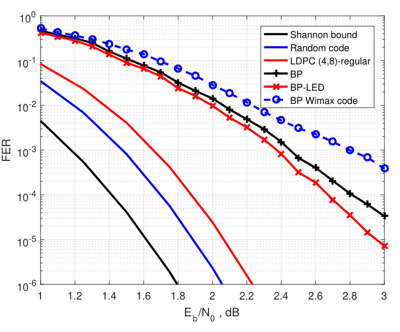 Figure 1
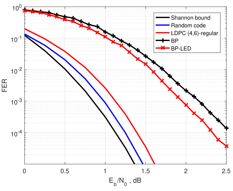 Figure 2
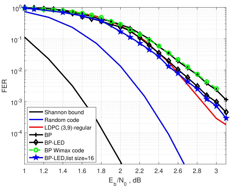 Figure 3
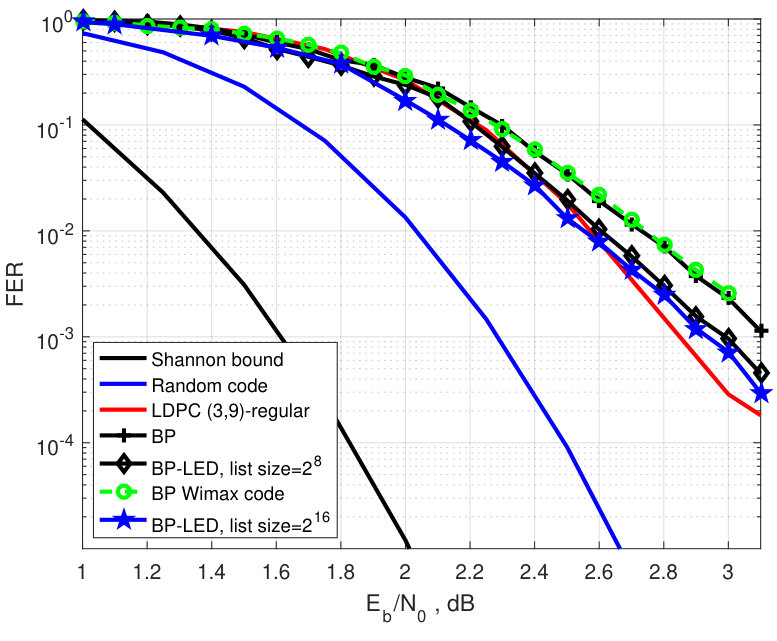 Figure 4
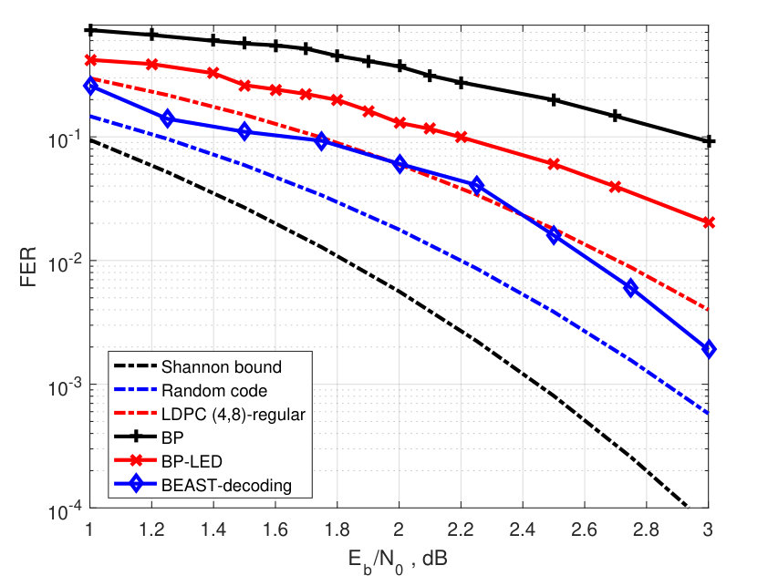 Figure 5
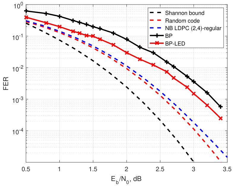 Figure 6
| Rate | 1/5 | 1/4 | 1/2 | 5/8 | 3/4 | |
|---|---|---|---|---|---|---|
| (4,5) | (3,4) | (4,8) | (3,8) | (3,12) | (4,16) | |
| 0.9995 | 0.994 | 0.994 | 0.975 | 0.944 | 0.984 | |
Peer Reviews
No public reviews on file for this paper yet. If you reviewed it on a platform where reviews are public (OpenReview, ICLR, NeurIPS, ICML), you can paste yours below so the community can read it here.
Videos
No videos yet. Explain this paper in a talk, walkthrough, or lecture? Add one.
BP-LED decoding algorithm for LDPC codes over AWGN channels
**Irina E. Bocharova1,2, Boris D. Kudryashov1, Vitaly Skachek2,
and Yauhen Yakimenka2**
1 Department of Information Systems 2 Institute of Computer Science
St. Petersburg University of Information Technologies, University of Tartu
Mechanics and Optics Tartu 50409, Estonia
St. Petersburg 197101, Russia Email: { vitaly, yauhen } @ut.ee
Email: [email protected], [email protected]
Abstract
A new method for low-complexity near-maximum-likelihood (ML) decoding of low-density parity-check (LDPC) codes over the additive white Gaussian noise channel is presented. The proposed method termed belief-propagation–list erasure decoding (BP-LED) is based on erasing carefully chosen unreliable bits performed in case of BP decoding failure. A strategy of introducing erasures into the received vector and a new erasure decoding algorithm are proposed. The new erasure decoding algorithm, called list erasure decoding, combines ML decoding over the BEC with list decoding applied if the ML decoder fails to find a unique solution. The asymptotic exponent of the average list size for random regular LDPC codes from the Gallager ensemble is analyzed. Furthermore, a few examples of regular and irregular quasi-cyclic LDPC codes of short and moderate lengths are studied by simulations and their performance is compared with the upper bound on the LDPC ensemble-average performance and the upper bound on the average performance of random linear codes under ML decoding. A comparison with the BP decoding performance of the WiMAX standard codes and performance of the near-ML BEAST decoding are presented. The new algorithm is applied to decoding a short nonbinary LDPC code over the extension of the binary Galois field. The obtained simulation results are compared to the upper bound on the ensemble-average performance of the binary image of regular nonbinary LDPC codes.111Results of this work were partly published in[1]. This work is supported by the Norwegian-Estonian Research Cooperation Programme through the grant EMP133.
I Introduction
Since their rediscovery in 1995, low-density parity-check (LDPC) codes in conjunction with iterative decoding continue to attract attention of both researches and companies developing communication standards. The main reason for this popularity of LDPC codes is their near-Shannon limit performance. Although there exist asymptotic ensembles of LDPC codes approaching capacity under belief propagation (BP) decoding, performance of finite length LDPC codes under BP decoding is inferior to their performance under maximum-likelihood (ML) decoding. Moreover, the performance gap between ML and BP decoding increases when signal-to-noise ratio (SNR) grows. Typically, LDPC codes under BP decoding suffer from the so-called error floor phenomen, which is caused by both sub-optimality of the decoding algorithm and by structural properties of the codes.
There exists a variety of techniques for lowering the error floors, and they are usually based on identifying and removing specific structural configurations of the code Tanner graph called trapping sets [2]. This can be done by modifying both the code parity-check matrix (without changing the code) and the iterative decoding algorithm. For example, in [3], a list of trapping sets is computed and stored in a look-up table. If the BP decoder fails, then a post-processing based on the list of known trapping sets is performed. Techniques combining the trapping set detection with code shortening or bit-pinning are presented in [4] and [5]. A technique based on eliminating small trapping sets by adding extra checks to the code parity-check matrix is studied in [6]. A method for eliminating small trapping sets when constructing an LDPC code is considered in [7]. The proposed method is applicable to both regular and irregular LDPC codes.
Another approach for improving the performance of BP decoding stems from the information set decoding. The most efficient methods for near-optimal decoding of linear codes are based on multiple attempts for finding an error-free information set and subsequent reconstruction of a codeword by re-encoding [8, 9, 10]. In [11] and [12], a post-processing in the form of bit-guessing is applied to the output of the BP decoder in case of its failure. In particular, in [11], the bits that participate in the largest number of unsatisfied checks are guessed, and BP decoding is repeated for each guessing attempt. An improved algorithm for selecting the bits to be guessed is suggested in [12]. There, the post-processing step is performed in stages. That technique leads to better than in [11] performance of near-ML decoding at the cost of higher computational complexity. A method for decoding of nonbinary LDPC codes over extensions of the binary Galois field based on the ordered statistics approach [10] is studied in [13].
Reconstruction of a codeword from a susbet of its symbols is equivalent to decoding over a binary erasure channel (BEC). It was shown in [14] that ML decoding of an LDPC code (where is the code length and is the number of the information symbols) with erasures is equivalent to solving a system of linear equations of order , that is, it can be performed via the Gaussian elimination with time complexity at most . By taking into account the sparsity of the parity-check matrix of the codes, the complexity can be lowered to approximately (see overview and analysis in [15] and the references therein). Practically feasible algorithms with thorough complexity analysis can be found in [16].
Low-complexity suboptimal decoding techniques for LDPC codes over a BEC are often based on the following two approaches. In the first approach, redundant rows and columns are added to the original code parity-check matrix (see, for example, [17],[18]). In the second approach, a post-processing is used in case BP decoding fails [19, 20, 21].
The idea to reduce the problem of the decoding of an LDPC code over the AWGN channel to the decoding of erasures has first appeared in [22]. In that work, BP decoding is followed by introducing artificial erasures and their subsequent decoding over the BEC, thus yielding a near-ML decoding algorithm. The performance of the decoding algorithm in [22] strongly depends on the efficiency of the procedure that converts the AWGN channel into the BEC or, in other words, the procedure for selecting the bits, which are to be erased. The channel transformation can be considered successful only if non-erased bits of the input vector are error-free.
In this paper, we propose a new decoding algorithm, which uses the ideas similar to [22] and [11], but differs significantly both in a strategy for introducing erasures and in an erasure decoding algorithm. A new list erasure decoding (LED) algorithm, which is applied to the result of the BP decoding in case of its failure can, in principle, be combined with any type of soft decoding on the AWGN channel. A distinguishing feature of the LED algorithm is an additional search step over a fixed size list of unresolved bit positions which is applied if the ML decoder over the BEC fails to find a unique solution. The proposed algorithm which we call BP-LED decoding is tested on the regular quasi-cyclic (QC) LDPC code with optimized girth of the code Tanner graph [23] and on the irregular QC LDPC codes optimized by using the technique in [24]. Both binary LDPC codes and binary images of nonbinary LDPC codes are studied. Simulation results are presented. The comparison with the theoretical bounds on the ML decoding performance is performed.
The rest of the paper is organized as follows. Some necessary definitions are given in Section II and known bounds on the error probability of ML decoding are revisited in Section III. List-decoding algorithm over the BEC is described in Section IV and its analysis for the Gallager ensemble of regular LDPC codes is presented in Section V. Techniques for selecting bit positions to be erased are discussed in Section VI. The near ML decoding procedure using LED is described in Section VII. The paper is concluded by the discussion of the simulation results and their comparison with the bounds on the error probability of ML decoding in Section VIII.
II Preliminaries
Consider the Gallager ensemble of -regular LDPC codes of length and dimension [25]. In this ensemble, an random parity-check matrix that consists of strips {\mbox{\boldmathH}}_{i} of width rows each, , where . All strips are random column permutations of the strip where the th row contains ones in positions , for .
Rate QC LDPC codes are determined by a polynomial parity-check matrix of their parent convolutional code [26]
[TABLE]
where is either zero or a monomial entry, that is, with being a nonnegative integer, , and is the syndrome memory. The polynomial matrix (5) can be represented via the degree matrix
[TABLE]
with entries at the positions of the monomials . We write for the positions where . By tailbiting the parent convolutional code to length , we obtain the binary parity-check matrix (see [26, Chapter 2])
[TABLE]
of the QC LDPC block code of length and dimension , where {\mbox{\boldmathH}}_{i}, , are binary matrices in the series expansion
[TABLE]
and is the all-zero matrix of size . Further by we denote the all-zero matrix of an appropriate size. If each column of {\mbox{\boldmathH}}(D) contains nonzero elements, and each row contains nonzero elements the QC LDPC block code is -regular. It is irregular otherwise.
Another form of the equivalent binary QC LDPC block code can be obtained by replacing the nonzero monomial elements of {\mbox{\boldmathH}}(D) in (5) by the powers of the circulant permutation matrix , whose rows are cyclic shifts by one position to the right of the rows of the identity matrix.
The polynomial parity-check matrix {\mbox{\boldmathH}}(D) (5) can be interpreted as a binary base matrix labeled by monomials, where the entry in is one if and only if the corresponding entry of {\mbox{\boldmathH}}(D) is nonzero, i.e.
[TABLE]
By viewing as a biadjacency matrix [27], we obtain a corresponding bipartite Tanner graph. The girth is the length of the shortest cycle in the Tanner graph.
III Tightened Bounds on the ML decoding error probability
In what follows, we compare the performance of the new decoding algorithm with the performance of ML decoding over an AWGN channel. While keeping that in mind, in this section we revisit known bounds on the error probability of ML decoding over the AWGN channel.
By using technique in [28] we compute the exact spectrum coefficients for the Gallager ensembles of binary regular LDPC codes and binary images of nonbinary regular LDPC codes. By substituting the computed coefficients into the existing bounds on the error probability of ML decoding, we obtain new bounds, which are tighter than the previously known counterparts.
III-1 Lower bound
Since 1959, the Shannon bound [29] is still the best known lower bound on the ML decoding error probability for codes used over the AWGN channel in a wide range of rates and lengths [30]. Computational aspects of this bound are studied in [31] (see also [30] for overview of the results in this area). In the sequel, we use approximation in [32] of the Shannon bound [29] which gives values indistinguishable from the values of the bound in [29] for the frame error rate (FER) performance below 0.1 over the AWGN channel.
Let , , and denote the code length, code rate and standard noise deviation for an AWGN channel, respectively. We use notations and formulas in [29] for the cone half-angle , which corresponds to the solid angle of an -dimensional circular cone, and for the solid angle of the whole space
[TABLE]
respectively. For a given code of length and cardinality , the parameter is selected as a solution of the equation
[TABLE]
Then, for the FER , we use approximation in [32]
[TABLE]
where .
III-2 Upper bound
The tangential sphere bound (TSB) (also known as the Poltyrev upper bound [33]) is based on Gallager’s bounding technique. Given a transmitted vector, the decoding FER is represented in the form
[TABLE]
where is a decoding error event, is the received vector and denotes the region, whose choice significantly influences the tightness of the bound (9). The tightest bound in [33] uses a conical region . It combines the ideas of spherical approach [34], which considers a spherical regions , and the tangential bound [35], which decomposes the noise vector into the radial and tangential components. We present here the Poltyrev bound [33] for completeness:
[TABLE]
Here is the Gaussian probability density function, ,
[TABLE]
is the -th spectrum coefficient of the code weight spectrum, is the code length, and denotes the probability density function of chi-squared distribution with degrees of freedom.
Parameter is a solution with respect to of the equation
[TABLE]
[TABLE]
We note that in order to use the Poltyrev bound (10), one has to know the weight spectrum of the code.
In what follows, we use the exact coefficients of the average spectrum of the Gallager ensemble of LDPC codes computed by the recurrent procedure presented in [28]. Let
[TABLE]
be a parity-check matrix of an LDPC code randomly chosen from the Gallager ensemble. In our derivations we use the generating function of a sequence of code weight enumerators. In a general case, the generating function for a sequence of numbers is defined as follows:
[TABLE]
where is a formal variable.
The generating function of the number of binary sequences of weight and length satisfying the equality
[TABLE]
where , is given by
[TABLE]
where , if is even, and otherwise.
From (13), we obtain the recurrent relation
[TABLE]
The probability that (12) is valid for a random of length and weight is equal to
[TABLE]
for each of the matrices {\mbox{\boldmathH}}_{i}. The average number of codewords of length and weight is given by
[TABLE]
where \big{(}p(w)\big{)}^{J} is the probability that satisfies (12) for all simultaneously, and E{ } denotes the expected value of a random variable.
Similarly, average spectra for binary images of nonbinary LDPC codes over , can also be computed via the generating function
[TABLE]
where (see [25, Chapter 5]) and
[TABLE]
(see [28] for details).
IV List Decoding over a BEC
Let {\mbox{\boldmathH}}=\left(\boldsymbol{h}_{1},\boldsymbol{h}_{2},\dots,\boldsymbol{h}_{n}\right) be an parity-check matrix of a binary linear block code, , where denotes the -th column of . We use notation {\mbox{\boldmathH}}_{I} for the submatrix of , whose columns are indexed by the set .
Consider a BEC with erasure probability . The ML decoder corrects any pattern of erasures if . If then the ML decoder can correct some erasure patterns. The number of such correctable patterns depends on the code structure.
Let be a received vector, where , and the symbol represents erasures. We denote by a binary vector, such that
[TABLE]
for all . Let be a set of nonzero coordinates of , , and be a vector of unknowns located in positions indexed by the set . Let be the vector with unknowns in positions .
Consider a system of linear equations \tilde{\boldsymbol{y}}{\mbox{\boldmathH}}^{\rm T}=\boldsymbol{0} which can be reduced to
[TABLE]
where \boldsymbol{s}(\boldsymbol{e})=\boldsymbol{y}_{I^{\rm c}(\boldsymbol{e})}{\mbox{\boldmathH}}^{\rm T}_{I^{\rm c}(\boldsymbol{e})} is a syndrome vector computed using non-erased positions of and
[TABLE]
The solution of (22) is unique if \rho\triangleq{\rm rank}{\mbox{\boldmathH}}_{I(\boldsymbol{e})}{=\nu}, otherwise the full list of candidate solutions contains elements, where
If the code rate approaches the BEC capacity , the typical number of erasures . In that case, with high probability, the dimension of the linear space of solutions of (22) is positive.
If , by using Guassian elimination and column and row permutations, the submatrix {\mbox{\boldmathH}}_{I(\boldsymbol{e})} can be represented in the form shown in Fig. 1. Here, by we denote the rank of the system of linear equations left after Gaussian elimination. It is easy to see that the first positions are uniquely determined and the other positions satisfy equations and cannot be determined uniquely. By assigning arbitrarily values to of these positions, we uniquely determine the remaining positions. A set of the corresponding columns of the submatrix is called arbitrarily assigned (AA) positions.
Definition 1**.**
*List erasure decoder (LED) is a decoder for the BEC, which for a given input with erased positions, outputs a list of codewords coinciding with the input word on all non-erased coordinates. *
A possible implementation of the LED is presented as Algorithm 1. In this algorithm, a row is called a pivot if it is chosen to eliminate nonzero elements in other rows in a position which we call a leader.
The algorithm combines BP decoding over the erasure channel and the Gaussian elimination steps. While there exists a row with one erasure, the BP decoding step is performed. If there are no rows with one erasure, and there is a row which was not used as a pivot yet, the Gaussian elimination step with respect to the leader is performed. Then, the algorithm switches back to the BP decoding step. These alternating steps are performed until neither rows with one erasure nor unused pivots are left.
V Analysis of the LED algorithm
As it is mentioned in Section II, we consider the Gallager ensemble of random -regular LDPC codes. A random parity-check matrix which determines an -regular LDPC code from this ensemble can be represented in the following form:
[TABLE]
where
[TABLE]
is of size , , and all the matrices {\mbox{\boldmathH}}_{i}, , are random permutations of the columns of {\mbox{\boldmathH}}_{1}.
In this section, we estimate the average size of the list of candidate solutions in the system (22). Denote by a random variable, which represents this number of solutions. A set of solutions of
[TABLE]
represents a coset of solutions of (22). Next we analyze (33) instead of (22) since all cosets have the same number of solutions. Denote by {\mbox{\boldmathH}}_{I(\boldsymbol{e}),1} a submatrix of {\mbox{\boldmathH}}_{I(\boldsymbol{e})} of size consisting of its first rows. Next, we state the following lemma.
Lemma 1:
Consider the Gallager ensemble of -regular binary LDPC codes of length and redundancy over the BEC with erasure probability . Then, the conditional probability that a row in {\mbox{\boldmathH}}_{I(\boldsymbol{e}),1} has zero weight given that there are erasures and rows have zero weight does not grow with and is upper-bounded by .
Proof.
Let denote the weight of the -th row of {\mbox{\boldmathH}}_{I(\boldsymbol{e}),1}, where . Then, the probability that the -th row has zero weight given that erasures occurred can be estimated as
[TABLE]
The conditional probability that rows of {\mbox{\boldmathH}}_{I(\boldsymbol{e}),1} have weight zero is given by:
[TABLE]
where .
It is easy to see that
[TABLE]
where the last transition is due to
[TABLE]
We conclude that the probability in (36) does not grow when the number of conditions increases, that is the following chain of inequalities holds
[TABLE]
[TABLE]
In what follows, we present the main theoretical result of this work.
Theorem 1:
Consider the Gallager ensemble of -regular binary LDPC codes of length and redundancy over the BEC with the erasure probability . If there are erasures, then the ensemble average list size in LED, , is upper-bounded by
[TABLE]
Proof.
Consider a random vector
[TABLE]
Let , , be an arbitrary set of indices. Denote by a subvector of components of the vector indexed by .
If erasures occurred, then the probability that the random vector is a solution of the system \boldsymbol{z}{\mbox{\boldmathH}}_{I(\boldsymbol{e}),1}^{\rm T}=\boldsymbol{0} can be represented in the following form
[TABLE]
where .
For the choice of a random vector and a random parity-check matrix from the Gallager ensemble, the probability of a zero syndrome component is
[TABLE]
where . It follows from (39) that
[TABLE]
[TABLE]
By substituting (39) into (40), and by applying Lemma 1, we obtain
[TABLE]
In what follows, we show that
[TABLE]
Consider the probability , , . By using the arguments similar to those in (41), it is easy to obtain
[TABLE]
The conditional probability in the RHS of (42) can be represented as
[TABLE]
[TABLE]
Substitution of (39) into (43) yields
[TABLE]
In (44), we took into account that .
Since does not depend on , from (44), by using Lemma 1 and (41), we obtain
[TABLE]
[TABLE]
From the last inequality and (42), we conclude that
[TABLE]
By using similar arguments it is easy to show that
[TABLE]
Then, from (38) we obtain
[TABLE]
Next, consider the submatrices {\mbox{\boldmathH}}_{I(\boldsymbol{e}),i}, , consisting of rows , respectively. Recall that the strips are obtained by the independent random permutations. If erasures occurred then the probability that a random vector is a solution of the system \boldsymbol{z}{\mbox{\boldmathH}}_{I(\boldsymbol{e})}^{\rm T}=\boldsymbol{0} is upper-bounded as
[TABLE]
Notice that analogous to the derivations in [25] we ignore the fact that parity-checks of {\mbox{\boldmathH}}_{I(\boldsymbol{e})} are linearly dependent. If is large enough (i.e. grows linearly with ) then a number of linearly dependent rows in {\mbox{\boldmathH}}_{I(\boldsymbol{e})} is of order and can be neglected.
Given that erasures occurred, we introduce a random variable which is equal to 1 if is a solution of \boldsymbol{z}{\mbox{\boldmathH}}_{I(\boldsymbol{e})}^{\rm T}=\boldsymbol{0}, and is equal to 0 otherwise. More formally,
[TABLE]
Then, the average list size (given that there are erasures) is equal to the average number of vectors which are solutions of \boldsymbol{z}{\mbox{\boldmathH}}_{I(\boldsymbol{e})}^{\rm T}=\boldsymbol{0}, namely
[TABLE]
Corollary 1:
Denote by the normalized number of erasures. The asymptotic exponent of the list size is determined by
[TABLE]
It is interesting to find a critical (largest) value of , such that or, in other words, to find the relative number of erasures such that the average list size does not exceed 1.
We expect that for sparse matrices it holds . Examples of critical values of for some code rates and for some values of are shown in Table I. We can see that is close to 1 even for rather sparse parity-check matrices. This suggests that the allowable fraction of erasures can be chosen close to .
VI Conversion of decoding over an AWGN channel into decoding over a BEC
In [22], the main criteria for bits to be erased is the number of unsatisfied parity checks and low bit reliability values. The authors present therein a set of thresholds which depend both on the code structure and on the channel signal-to-noise ratio (SNR). The corresponding bit is erased if the number of unsatisfied checks and the reliability value exceed the chosen thresholds.
We use a different strategy to transform the original problem of decoding over an AWGN channel into a decoding problem over a BEC. By taking into account that only iterations of BP decoding can be considered independent, we analyze bit reliability values obtained after iterations. This allows us to avoid overestimating the reliability values. An overview of various techniques for processing BP reliability values for their further use in the near-ML decoding can be found in [13]. In our approach, first we calculate the minimum absolute values of bit reliability values (over iterations). Next, we sort them in the increasing order. The least reliable bits are erased.
After erasing the least reliable bits, we introduce additional erasures by using a set of masks , where , and for . We use pseudo-random pre-selected binary sequences of length and weight as masks. In our simulations we used codewords of the first order Reed-Muller code , , as such masks. The masks are applied to the next least reliable entries (after positions have already been erased). This step in the algorithm is similar to the bit flipping step in the decoding algorithms such as [9, 10]. The choice of the parameters and depends on the code length and the code rate. In our simulations, we have chosen the total number of erasures to be:
[TABLE]
where . We found empirically that for the rate , for any code length, we can choose and .
The BP-LED decoding can also be applied to decoding of nonbinary LDPC codes over extensions of the Galois fields. It was found experimentally that for the -regular LDPC code of length 16 over (128 bits) constructed in [36], the choice gives the best FER performance. In our experiments, was chosen to be .
VII LED-based algorithm for an AWGN channel
In this section, we show how the LED can be used for decoding of LDPC codes on an AWGN channel with binary phase shift keying (BPSK) signaling. Let {\mathcal{C}}=\{{\mbox{\boldmathc}}_{j}\}_{j=0,1,\cdots,2^{k}-1} be a binary LDPC code. Assume that is used with BPSK and coherent detection to communicate over an AWGN channel. The binary code symbol is mapped onto the signal , , where is the signal energy. In the sequel we assume that . Thus the codewords , , are mapped onto bipolar sequences . Assume that is transmitted. Then the discrete-time received signal is , where the noise vector consists of independent zero-mean Gaussian random variables with variance . The SNR per information bit is denoted by = , where is the code rate.
Assume that and are the transmitted and the received vectors, respectively. Let be the maximal number of allowed candidate solutions, and be a decoding metric. We use the Euclidean distance between the channel output and as the decoding metric , where is a candidate codeword. Alternatively, we can maximize the scalar product of and .
The new BP-LED decoding algorithm is presented as Algorithm 2.
In Algorithm 2, first, input symbols are erased (see below). Then LED is used for correcting of erasures and for making a list of the AA positions.
The high-level idea of the proposed decoding algorithm is as follows. The algorithm consists of the three main steps:
BP decoding. 2. 2.
In case of BP decoding failure, the unreliable positions are erased and LED is applied. 3. 3.
In case of the LED failure to find a unique solution, exhaustive search over a list of candidate codewords is carried out.
These three steps are implemented as the following three subroutines in Algorithm 2.
- •
, where and are vectors of hard decisions and of symbol reliabilities, respectively, produced by the BP decoder. As it is mentioned above, in order to avoid overestimates due to cycles in the Tanner graph, is computed as the minimum of the absolute values of the symbol reliabilities in the first iterations.
- •
, where is a vector with zeros on erased positions, and is a vector of hard decisions with erasures in AA positions. Function LED is as discussed in Section IV.
- •
. This subroutine generates the -th candidate codeword from the full list of solutions of (22). This is done by constructing a list of binary words of length ordered according to the ascending order of their weights. Then, the -th candidate is obtained by flipping AA bits in positions determined by the ones of the -th element in .
VIII Discussion and Simulation results
In this section, we compare experimentally the FER performance of BP decoding (with 50 decoding iterations) with that of the BP-LED decoding. We also compare the experimental results with the tightened theoretical upper bounds for binary random linear codes and for the Gallager ensembles of binary reqular LDPC codes and binary images of nonbinary regular LDPC codes under ML decoding. Specifically, we simulate the rate binary irregular LDPC codes of length and the rate binary -regular LDPC code of length . We also simulate the LED-based decoding for the rate nonbinary LDPC code of length over [36] and compare its performance with the FER performance of the generalized BP decoding [37] of the same code, and with the corresponding theoretical upper and lower bounds.
The experimental results are shown in Fig. 6. While simulating the BP- LED decoding for nonbinary codes over extensions of the binary field we recomputed probabilities of bit values via probabilities of symbol values of , , as follows
[TABLE]
where is the probability of the -ary symbol to be equal , , , is the probability that the -th bit in the binary representation of is equal to , and
is the binary representation of .
All parity-check matrices of the simulated binary irregular LDPC codes were constructed by using the optimization technique in [24]. The parity-check matrix of the -binary regular code was obtained by reducing modulo 6 the degree matrix of the double Hamming LDPC code in [23]. In order to show that the chosen codes are on a par with the best LDPC codes used in communication standards, the FER performance of BP decoding for the standard WiMAX codes of rates and is presented in Figs. 2 and 3. To facilitate the low complexity encoding, the degree matrices of all simulated codes of length have the so-called bi-diagonal form. The FER performance of the LDPC code was compared with the FER performance of near-ML BEAST-decoding [38].
In the simulations of the binary LDPC codes, the parameters and were optimized over the range and , respectively. Among the erased positions, positions were selected according to the reliabilities, estimated by the BP decoding, and positions were selected pseudo-randomly from the next less reliable positions. Two values of the sizes of the pseudo-random sets, and , as well as two values of the list sizes, and , were simulated. All the simulations were run until at least 100 LED-decoding block errors occurred. It turns out that for all codes, except for the rate irregular LDPC code, two sets of parameters: and the list size ; and the list size ,— provide approximately the same coding gain of the LED-based algorithm with respect to the BP decoding. For the rate code, the LED-based algorithm with a larger list size yields a slightly lower FER. In nonbinary case, the parameter is selected, the number of trials is and the list size is .
In order to compare the FER performance of the BP-LED decoding of both regular and irregular LDPC codes with the FER performance of ML decoding, in Figs. 2–5 we present an upper bound (10) computed for both the random linear codes and for the -regular LDPC codes from the Gallager ensemble. In case of irregular LDPC codes, the upper bound is computed for the parameters and chosen to be equal to the average number of ones in columns and rows of the parity-check matrix, respectively. The Shannon lower bound (8) is presented in the same figures as well. From the presented results, we conclude that the coding gain is higher for the regular code than for the optimized irregular LDPC codes. We also observe that for binary codes the coding gain grows with . For higher rates, the FER performance of the LED-based algorithm is closer to the corresponding upper bound on ML decoding performance than for lower rates. It is easy to see that the coding gain compared to the FER performance of BP decoding for the rate WiMAX code is significant. However, the rate WiMAX code has the same FER performance as the optimized LDPC code. For the -regular LDPC code of length , the coding gain of the new algorithm with respect to the BP decoding is approximately two times smaller than the coding gain obtained by the near-ML BEAST decoding. In nonbinary case, the coding gain does not grow with . Such behavior of the FER performance can be explained by using LED in combination with generalized BP decoding which is superior to conventional BP decoding. Higher efficiency of generalized BP decoding reduces the gap in the FER performance of ML and BP decoding. As a result near-ML decoding provides a smaller coding gain than that for the binary LDPC codes.
The analysis of computational complexity of Steps 4 and 5 of Algorithm 2 is presented in [1]. Although for a general linear code, the computational complexity of Step 4 would be a cubic function of the code length , the empirically observed average decoding time for LDPC codes grows near-linearly with the code length. The computational complexity of Step 5 is proportional to the list dimension , that is, it grows linearly with the code length as well.
Although complexity grows near-linearly, the algorithm loses efficiency for large since a typical number of AA positions grows as well. To maintain the decoding efficiency, parameters and should also be increased, which leads to impractically high computational time for lengths above 2000.
IX Conclusion
A new algorithm for near-ML decoding of LDPC codes over the AWGN channel is proposed and analyzed. The new algorithm as well as BP decoding are simulated for both the regular and irregular binary QC LDPC codes of several rates and for the binary image of a short nonbinary LDPC code over the extension of the binary Galois field. The FER performance for binary and nonbinary LDPC codes is compared to the improved union-type upper bound on the error probability based on precise coefficients of the average spectra for the Gallager ensembles of binary regular LDPC codes and binary images of nonbinary regular LDPC codes, respectively. The coding gain of the new decoding algorithm strongly depends on the communication scenario. Decoding performance close to the performance of ML decoding is demonstrated for the high rate LDPC codes as well as for the short length LDPC codes.
The reference list from the paper itself. Each links out to its DOI / PubMed record.
- 1[1] I. E. Bocharova, B. D. Kudryashov, V. Skachek, and Y. Yakimenka, “Low complexity algorithm approaching the ML decoding of binary LDPC codes,” in IEEE Int. Symp. on Inform. Theory (ISIT) , 2016, pp. 2704–2708.
- 2[2] T. Richardson, “Error floors of LDPC codes,” in 41st Allerton Conf. on Communication, Control and Computing , 2003.
- 3[3] E. Cavus and B. Daneshrad, “A performance improvement and error floor avoidance technique for belief propagation decoding of LDPC codes,” in IEEE 16th Int. Symp. on Personal, Indoor and Mobile Radio Commun. (PIMRC) , vol. 4, 2005, pp. 2386–2390.
- 4[4] Y. Han and W. E. Ryan, “Low-floor decoders for LDPC codes,” IEEE Trans. Commun. , vol. 57, no. 6, pp. 1663–1673, 2009.
- 5[5] Y. Zhang and W. E. Ryan, “Toward low LDPC-code floors: a case study,” IEEE Trans. Commun. , vol. 57, no. 6, pp. 1566–1573, 2009.
- 6[6] M. Jianjun, J. Xiaopeng, L. Jianguang, and S. Rong, “Parity-check matrix extension to lower the error floors of irregular LDPC codes,” IEICE Trans. on Commun. , vol. 94, no. 6, pp. 1725–1727, 2011.
- 7[7] R. Asvadi, A. H. Banihashemi, and M. Ahmadian-Attari, “Lowering the error floor of LDPC codes using cyclic liftings,” IEEE Trans. Inform. Theory , vol. 57, no. 4, pp. 2213–2224, 2011.
- 8[8] E. Prange, “The use of information sets in decoding cyclic codes,” IRE Trans. Inform. Theory , vol. 8, no. 5, pp. 5–9, 1962.