Fundamental precision limit of a Mach-Zehnder interferometric sensor when one of the inputs is the vacuum
Masahiro Takeoka, Kaushik P. Seshadreesan, Chenglong You, Shuro Izumi,, Jonathan P. Dowling

TL;DR
This paper clarifies the conditions under which a Mach-Zehnder interferometer with vacuum input can surpass the shot noise limit, revealing that the no-go theorem does not apply when only one arm contains the unknown phase shift.
Contribution
The paper rigorously analyzes the no-go theorem in quantum metrology, showing it does not hold when the phase shift is localized in a single arm of the interferometer.
Findings
The no-go theorem applies only when the phase shift is split between both arms.
An explicit measurement strategy is provided that beats the shot noise limit.
The two sensing scenarios are physically distinct and have different implications.
Abstract
In the lore of quantum metrology, one often hears (or reads) the following no-go theorem: If you put vacuum into one input port of a balanced Mach-Zehnder Interferometer, then no matter what you put into the other input port, and no matter what your detection scheme, the sensitivity can never be better than the shot noise limit (SNL). Often the proof of this theorem is cited to be in Ref. [C. Caves, Phys. Rev. D 23, 1693 (1981)], but upon further inspection, no such claim is made there. A quantum-Fisher-information-based argument suggestive of this no-go theorem appears in Ref. [M. Lang and C. Caves, Phys. Rev. Lett. 111, 173601 (2013)], but is not stated in its full generality. Here we thoroughly explore this no-go theorem and give the rigorous statement: the no-go theorem holds whenever the unknown phase shift is split between both arms of the interferometer, but remarkably does not…
Click any figure to enlarge with its caption.
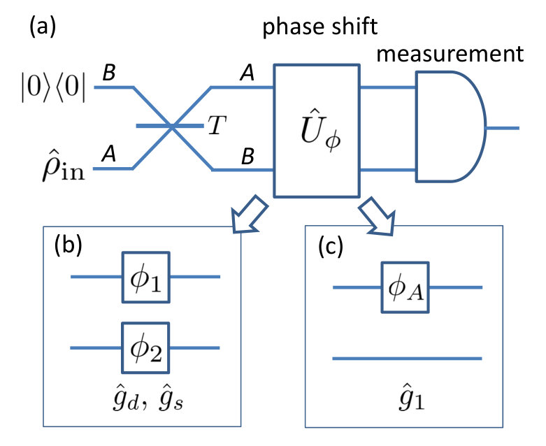 Figure 1
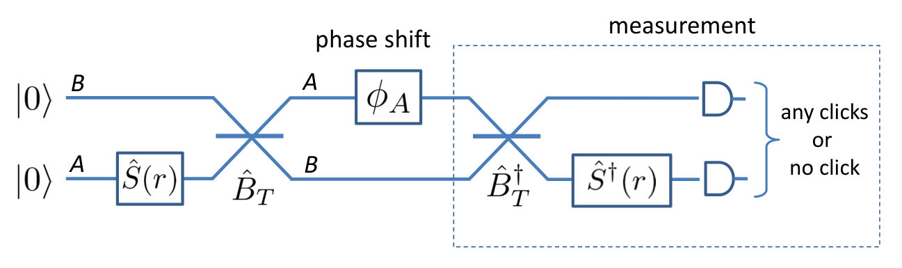 Figure 2
Peer Reviews
No public reviews on file for this paper yet. If you reviewed it on a platform where reviews are public (OpenReview, ICLR, NeurIPS, ICML), you can paste yours below so the community can read it here.
Videos
No videos yet. Explain this paper in a talk, walkthrough, or lecture? Add one.
Fundamental precision limit of a Mach-Zehnder interferometric sensor when one of the inputs is the vacuum
Masahiro Takeoka
National Institute of Information and Communications Technology, Koganei, Tokyo 184-8795, Japan
Kaushik P. Seshadreesan
Max Planck Institute for the Science of Light, 91058 Erlangen, Germany
Hearne Institute for Theoretical Physics and Department of Physics and Astronomy, Louisiana State University, Baton Rouge, Louisiana 70803, USA
National Institute of Information and Communications Technology, Koganei, Tokyo 184-8795, Japan
Chenglong You
Hearne Institute for Theoretical Physics and Department of Physics and Astronomy, Louisiana State University, Baton Rouge, Louisiana 70803, USA
Shuro Izumi
National Institute of Information and Communications Technology, Koganei, Tokyo 184-8795, Japan
Sophia University, 7-1 Kioicho, Chiyoda-ku, Tokyo 102-8554, Japan
Jonathan P. Dowling
Hearne Institute for Theoretical Physics and Department of Physics and Astronomy, Louisiana State University, Baton Rouge, Louisiana 70803, USA
Abstract
In the lore of quantum metrology, one often hears (or reads) the following no-go theorem: If you put vacuum into one input port of a balanced Mach-Zehnder Interferometer, then no matter what you put into the other input port, and no matter what your detection scheme, the sensitivity can never be better than the shot noise limit (SNL). Often the proof of this theorem is cited to be in Ref. [C. Caves, Phys. Rev. D 23, 1693 (1981)], but upon further inspection, no such claim is made there. A quantum-Fisher-information-based argument suggestive of this no-go theorem appears in Ref. [M. Lang and C. Caves, Phys. Rev. Lett. 111, 173601 (2013)], but is not stated in its full generality. Here we thoroughly explore this no-go theorem and give the rigorous statement: the no-go theorem holds whenever the unknown phase shift is split between both arms of the interferometer, but remarkably does not hold when only one arm has the unknown phase shift. In the latter scenario, we provide an explicit measurement strategy that beats the SNL. We also point out that these two scenarios are physically different and correspond to different types of sensing applications.
Introduction.— In the field of quantum metrologyGiovannetti et al. (2011); Demkowicz-Dobrzaǹski et al. (2015); Dowling and Seshadreesan (2015), a Mach-Zehnder interferometer (MZI) is a tried and true workhorse that has the additional advantage that any result obtained for it also applies to a Michelson interferometer (MI) and hence has a potential application to gravitational wave detection. In most current implementations of gravitational wave detectors, the MI is fed with a strong coherent state of light in one input port and vacuum in the other (Fig. 1). It was in this context that Caves in 1981 Caves (1981) showed that such a design would always only ever achieve the shotnoise limit (SNL). Then he showed if you put squeezed vacuum into the unused port, you could beat the SNL. Several implementations of this squeezed vacuum scheme have already been demonstrated in the GEO 600 gravitational detector, and plans are underway to utilize this approach in the LIGO and VIRGO detectors in the future Grote et al. (2013); Lugiato et al. (2002).
It then appeared, that in the lore of quantum metrology, this result was extended — without proof — to the following no-go theorem: If you put quantum vacuum into one input port of a balanced MZI, then no matter what quantum state of light you put into the other input port, and no matter what your detection scheme, the sensitivity can never be better than the SNL. Often the proof of this theorem is cited to be the original 1981 paper by Caves Caves (1981), but upon further inspection, no such general claim is made there. A quantum-Fisher-information-based argument suggestive of this no-go theorem appeared in Ref. Lang and Caves (2013) by Lang and Caves, but it does not explore the statement in adequate generality.
In this work, we give a full statement of the no-go theorem. The statement proved here is the following: if the unknown phase shifts are in both of the two arms of the MZI, then the no-go theorem holds no matter whether the MZI is balanced or not. However, in the case where the unknown phase shift is in only one arm of the MZI, then the no-go theorem does not necessarily hold. The former is a multiparameter measurement and the latter is a single parameter. For the latter, we show an explicit scheme with a probe and measurement that can beat the SNL in the sense that its classical Fisher information (CFI) is proportional to the square of the total photon number used at the input and the measurement. The underlying issue is that two different models for the unknown phase shift unitary operation in the MZI can give different values of the QFI Jarzyna and Demkowicz-Dobrzański (2012); Pezzè et al. (2015). Since only the phase difference is utilized in both models, it has been thought that this discrepancy is a flaw in the interpretation of the QFI Jarzyna and Demkowicz-Dobrzański (2012) or is related to the assumptions of the input states and the measurements Pezzè et al. (2015). By contrast, here we point out that the different unitaries correspond to physically different types of sensors, and their choice should depend on the concrete application scenarios. Also for the former scenario (i.e. unknown phase shifts in two arms), we show that one has to carefully consider the phase sum (often regarded as the “global phase” though) whereas only phase difference is the quantity of interest. In other words, it is intrinsically a two-parameter estimation problem.
Related to the above, we also point out the pitfalls of using only the quantum Fisher information (QFI), or the closely related quantum Cramér-Rao (QCRB) bound Helstrom (1976), to make claims of a quantum metrological advantage, without explicitly providing a detection scheme that would actually achieve that advantage Jarzyna and Demkowicz-Dobrzański (2012). Before the QFI approach came into vogue in recent years, often theorists would try to optimize the input state and the detection scheme simultaneously. This often led to input states and detection schemes difficult to implement. The QFI approach freed us from having to optimized over all detection schemes, more accurately over all Positive Operate Valued Measures (POVM), but that freedom, carried a very high cost. The issue is that the optimal POVM that achieves the QFI may be difficult to implement or contain hidden resources, such as a strong local oscillator, that are not fairly counted as far as a quantum advantage is concerned Jarzyna and Demkowicz-Dobrzański (2012).
Quantum Fisher information approach to phase sensing— A schematic of the Mach-Zehnder (MZ) interferometer-type sensing we consider here is illustrated in Fig. 1(a). Two input modes A and B are interfered via a beam splitter with transmittance , and then put into the phase shift unitary operation followed by some measurement. In addition to this standard setting, we restrict one of the input states to always be the quantum vacuum state, whereas the other input can be an arbitrary quantum state (possibly mixed).
A similar setup to the one we consider here has recently used by Lang and Caves Lang and Caves (2013), where the two input ports are assumed to be in an arbitrary pure state and a coherent state , and the beam splitter transmittance is chosen to be 50/50 (i.e. ). The phase shift unitary operator is , where and are the phase sum and difference of the two modes, respectively, , . These two phase shift parameters reflect the unknown phase shifts in the two arms of the MZI, and , as , (see Fig. 1(b)). () and () are creation and annihilation operators in mode (), respectively.
Then the authors showed that for a coherent state input with , i.e. for the vacuum input, the quantum Fisher information (QFI) for the phase difference turns out to be the average photon number of the input:
[TABLE]
where . This result suggests that the precision of the phase sensing is shot-noise limited, when one of the input ports contains only vacuum (and the other mode contains any pure state), since the QCRB is .
However, the above result does not answer questions such as whether the no-go theorem still holds when the interferometer is not balanced, or when the phase shift unitary operator is chosen differently. Firstly, for the phase shift unitary operator , when deviates from , the QCRB already appears to beat the SNL. Keeping as a free parameter, and using the fact that the QFI of a pure state in estimating a phase shift generated by a generator is given by , we arrive at
[TABLE]
(See Supplemental Material 1 for the derivation.) This beats the SNL for any non-50/50 beam splitter quite spectacularly. For example, with , the QCRB approaches for some inputs such as squeezed vacuum Anisimov et al. (2010).
Secondly, as pointed out and rigorously discussed in Ref. Jarzyna and Demkowicz-Dobrzański (2012), a different choice of the phase shift unitary can give a different value for the QFI. For example, in lieu of the phase shift operator , one can instead choose , where , such that phase shift is generated only in one arm. The QFI for the phase shift unitary operator is found to be
[TABLE]
where is the photon number variance of . (See Supplemental Material 1 for the derivation.) This is obviously different from Eq. (1), and again implies a sub-SNL result, since is possible for some inputs, as mentioned above.
These results extrapolated from Ref. Lang and Caves (2013) are thus perplexing, since seemingly, both Eqs. (2) and (3) suggest the possibility of sub-SNL precision phase sensing even with the vacuum input into one of the input ports.
Phase shift in both arms vs. in one arm in the MZI sensing— We point out that the above phase-shift unitary operators (Figs. 1(b) and (c)) have different physical meanings and their choice should depend on what type of application scenario is in your mind. For the gravitational wave detection application, and should be chosen since the two arms of the (Michelson) interferometer both have unknown phase shifts induced by the gravitational waves (Fig. 1(b)). Also some commonly used sensing devices such as a differential interference contrast microscope Nomarski (1955) should be modeled in the same way. (See also its quantum version Ono et al. (2013).)
On the other hand, the most primitive use of the Mach-Zehnder interferometer is to put a sample in one of the two arms to measure the corresponding phase shift. This configuration is also widely used as a simple and low-cost technology to measure the sample’s density distribution, pressure, temperature, etc. This type of sensor should be modeled by (Fig. 1(c)). Since these two models are physically different, they may lead to different outcomes in our problem; the MZI with vacuum in one input port. That is, they could have different fundamental precision limits with vacuum in one input port. We will rigorously analyze each model in the following.
Remedy: Full quantum Fisher information matrix treatment— The MZI sensing with the - model in its full generality is a two-parameter estimation problem since there are two unknown parameters, and , in the system (although usually only the phase difference is an interesting quantity to measure). Therefore, a two-by-two quantum Fisher information matrix (QFIM) is considered. The problem in Eq. (2) is in fact due to the ignorance of the phase sum 111In Ref. Lang and Caves (2013), the QFIM of the system considered was calculated. However, they reduce it to the single-parameter estimation (i.e. drop off the terms for ) which looses the tightness of the bound. Note that this problem does not appear in Eq. (1) since with , the non-diagonal term of the QFIM goes to zero and thus the problem reduces to two independent single-parameter estimations. Nevertheless, in Ref. Lang and Caves (2013), they also consider the non-vacuum input case where the bound may have some looseness. . In multi-parameter estimation, the QCRB is given by
[TABLE]
where is the covariance matrix of the estimator including both and , is the number of trials, and is the two-by-two QFIM:
[TABLE]
where and correspond to and . The first diagonal element of in Eq. (4) corresponds to the estimation limit of , which is explicitly given by
[TABLE]
For an arbitrary mixed quantum state, the QFIM is in general not easy to calculate. However, the optimal input state that maximizes is always given by a pure-state input. This is the consequence of the convexity of the QFIM: for ,
[TABLE]
holds. This can be proved by using the monotonicity of the QFIM under the completely positive trace preserving (CPTP) map Petz (1996); Petz and Ghinea (2010) and extending the proof of the convexity for the QFI Fujiwara (2001). (See Supplementary Material 2.) The statement basically says that a statistical mixture of the input states will never increase the QFIM and thus implies that the QFIM is maximized with a pure state input. The optimal pure state for the QFIM is also optimal for the multi-parameter QCRB (4) since the QFIM is a positive matrix and for positive matrices and , holds if and only if . That is, a statistical mixture of the input states will never increase the sensitivity for both single- and multiple-parameter estimation.
Therefore, by considering a pure input state , the elements of the QFIM are given by
[TABLE]
where takes and . These are explicitly given by
[TABLE]
where note that corresponds to Eq. (2). Inserting these into (6), we get
[TABLE]
where the minimum of the right hand side is obtained with as , which is the SNL, as it should be. That is, no matter how highly nonclassical the input state is, and no matter what POVM you deploy, the SNL cannot be surpasses for so long as the other input to the interferometer is the vacuum state. Thus, this result establishes the no-go theorem in a most general form, which includes the beam splitter transmissivity as a free parameter.
Phase shift in one arm ()— The model is a single-parameter estimation problem and thus (3) is directly applied to the QCRB, which suggests the sub-SNL sensitivity with high , that is, input states with high photon number fluctuation such as squeezed vacuum. Then as mentioned at the introduction, the QFI-only approach may have the pitfall that the optimal POVM attaining the QCRB could contain huge amount of hidden resources as pointed out by Jarzyna and Demkowicz-Dobrzański Jarzyna and Demkowicz-Dobrzański (2012). In other words one can fool oneself into thinking, via the QFI-only approach, that there is some quantum metrological advantage, where none actually exists.
There are two remedies. The first, and the one we recommend, is that if authors wish to claim a quantum metrological advantage from a QFI-only calculation, they then must provide a detection scheme that actually hits the related QCRB, so all resources hidden in the associated POVM may be then laid bare for all to see. (We should note that in Ref. Anisimov et al. (2010), the authors were careful to back up the QFI calculation by providing a detection scheme — the parity operator — that actually hits the QCRB.)
The second remedy, besides producing the POVM that hits the limit, is to rule out any external resource that might give some phase information to the measurement device. Such a “rule-out” protocol was introduced by Jarzyna and Demkowicz-Dobrzański Jarzyna and Demkowicz-Dobrzański (2012). They resolved this issue by introducing the idea of a phase-averaged input state, where the two-mode input state from the two input ports is averaged by a common phase shift, which preserves the relative phase between two modes, but does not allow any phase information to be brought in from the outside of the interferometer, e.g. from the measurement devices themselves (a similar discussion appeared in the context of superselection rule Pezzè et al. (2015)). Therefore, the QFI of the phase-averaged input gives the proper phase-sensing limit without any external phase reference. A simple way to understand the phase averaging is to think of it as a type of phase randomization akin to preparing a thermal state. A thermal state can be used in an MZI for SNL interferometry, even though it contains no coherence, because each photon — as in Dirac’s dictum — only ever interferes with itself. In this way the advantage of any hidden resource in the POVM is mitigated.
Here we apply these two remedies separately. First, we employ the phase-averaging approach to eliminate any hidden resource in the POVM. For the two input states, we consider a vacuum and an arbitrary quantum state with the density matrix of
[TABLE]
where is the -photon number state. Then the phase-averaged input is given by
[TABLE]
where , , and is a real positive number satisfying .
The state after the first beamsplitter of the MZI and the phase shifting is given by
[TABLE]
where
[TABLE]
By using the convexity of the QFI and noticing that and are orthogonal for , we have
[TABLE]
where
[TABLE]
(See Supplementary Material 3 for the detailed derivation.) The maximum in Eq. (18) is attained at , and is equal to , as it should be.
Consequently, the QFI for is given as
[TABLE]
where is the average photon number of , and thus we find that the phase sensitivity is lower bounded as
[TABLE]
That is, if the optimal POVM is not allowed to have external phase information, the estimation precision is limited by the shot-noise limit.
There is, however, one question remaining: if one is allowed to use some additional resource at the measurement, is it possible to surpass the SNL with respect to the total number of resources used at the input and the detection process? As our last result, we prove that the answer is affirmative by showing a concrete measurement scheme.
Figure 2 illustrates the concrete input state and the measurement. The input state is a single-mode squeezed vacuum, which is generated from vacuum by applying the squeezing operation , where is the squeezing parameter. The measurement is a time-reversed process, that is, it consists of the complex-conjugate beam splitter , anti-squeezing operation , and photon detectors that discriminate zero and non-zero photons (so-called on-off detectors). For simplicity of the analysis, we consider only two outcomes: zero photons in both detectors or other events, {} (photon number discrimination may further improve the performance but to simplify the discussion here, we leave it for a future work). Note that this mirror-image like detection strategy has been considered in the context of state discrimination Takeoka et al. (2003); Takeoka and Sasaki (2008) and also the phase estimation via coherent-state input Izumi et al. (2016). Since we need the phase information of the input state at the anti-squeezing process, this is a phase-sensitive measurement, and so the POVM has access to external phase information and the phase of the squeezer . The input average photon number is given by . Since the measurement device also uses the same amount of squeezing, the average photon number of the all resources are counted as (to consider the fundamental limitation, here we assume a unit efficiency parametric downconverter where is directly a function of the pump energy used for the converter).
The attainable precision limit (in the asymptotic limit, ) is specified by calculating its CFI Helstrom (1976); Hayashi (2006):
[TABLE]
where is the conditional probability of obtaining the measurement outcome for given and represent the photon detection outcome and , respectively.
is calculated by the characteristic function approach (e.g. Ref. Takeoka et al. (2015)), and the derived analytical expression of is complicated (see Supplementary Material 4). Taking the limit of , we get
[TABLE]
where we remind the reader that is the total resource used for the input state and the detection process. Thus we get the (classical) CRB around as
[TABLE]
which surpasses the SNL of the total resource for any . This example shows how a QFI-only calculation could contain hidden resources in the unknown optimal POVM, that are unfairly not counted. Here, by taking all resources into account, we conclude that it is possible to beat the SNL for the estimation if one uses an additional energy and phase resources at the detection.
Conclusions.— In this paper, we revisit the ultimate limit of the MZI sensing precision when an input into one port is vacuum. We show a full statement of the problem with a rigorous proof: the statement depends on your choice of the phase shift unitary operator— in other words, on the physical setup of your sensing application.
First, if both two arms of the MZI have different unknown phase shifts in your application (e.g. gravitational wave detection) and input vacuum in one port, then no matter what you put in the other port, and no matter what your detection scheme you deploy, you can never do better than the SNL in phase sensitivity. The statement holds even if the first beamsplitter of the MZI is non-50:50. The proof is based on the fact that it is intrinsically a two-parameter estimation problem although the phase sum is often treated as a “global phase” and ignored in real experiments. Intuitively, we see that the state after the phase shift is (where is a probe state before the phase shift) which clearly contains . This implies if one knows nothing about , the effective state should be randomized over which might give a different conclusion than that from the analysis considering only as a single-parameter estimation. This is why we need to take into account both and even for deriving the precision bound of only . This type of sensing includes the gravitational wave detection Grote et al. (2013); Lugiato et al. (2002), long-baseline interferometry Parazzoli et al. (2016), and differential interference contrast microscopy Nomarski (1955); Ono et al. (2013), for example. In these applications, if one input is vacuum, our result rules out the possibility of doing something “quantum” at the detector (such as putting in a squeezer or doing photon addition or subtraction) to beat the SNL.
Second, if only one of the MZI arms has an unknown phase shift in your application (sensing a sample placed at one arm of the MZI), the ultimate precision limit depends on the detector restriction. If you do not allow the detector to use any external phase reference and power resource, then the precision is limited by the SNL. However, if you allow the detector to use such resources, you can beat the SNL in terms of the total resource used at the input and detector. The explicit sensing scheme which uses squeezers for both input and detector is given. This type of sensing includes simple MZI devices measuring sample’s density, pressure, temperature, etc, and also LIDAR-type sensing Gard et al. (2016). In these applications, only if you put nonclassical light into at least one input port, is there a hope to beat the SNL by doing something quantum at the detector, even if the other port is vacuum.
I Acknowledgements
MT would like to acknowledge suport from the Open Partnership Joint Projects of JSPS Bilateral Joint Research Projects and the ImPACT Program of Council for Science, Technology and Innovation, Japan. KPS, and JPD would like to acknowledge support from the Air Force Office of Scientific Research, the Army Research Office, the National Science Foundation, and the Northrop Grumman Corporation. CY would like to acknowledge support from an Economic Development Assistantship from the the Louisiana State University System Board of Regents.
Appendix A Supplemental Material 1: Quantum Fisher information
for the Mach-Zehnder interferometer phase sensing with a vacuum input
Here we derive Eqs. (3), (2), and (9)–(11) in the main text. Consider as an input to the MZ interferometer. For the calculation, it is useful to expand in a coherent state basis:
[TABLE]
where is a coherent state with complex quadrature amplitude . Then the average photon number and the variance of the state are given by
[TABLE]
and
[TABLE]
where we use the fact that .
The state after the beam splitter with transmittance is given by
[TABLE]
where .
A.1 QFI with (Eq. (3))
The quantum Fisher information (QFI) is calculated from
[TABLE]
We have
[TABLE]
and
[TABLE]
In total, we have
[TABLE]
For , it is and thus we get Eq. (3).
A.2 QFIM for and [Eq. (2), (9)–(11)]
For pure states, the elements of the QFIM are given by
[TABLE]
where takes and .
Recall that and . Then we have
[TABLE]
Similarly, we have
[TABLE]
Also
[TABLE]
and similarly,
[TABLE]
By using the above results, we have
[TABLE]
[TABLE]
Appendix B Supplemental Material 2: Convexity of quantum Fisher
information matrix
Here we prove the convexity of the quantum Fisher information matrix (QFIM):
[TABLE]
for . Here , , and are (maybe mixed) quantum states where is a set of unknown parameters.
To begin with, we briefly review the definition and the structure of the QFIM that we will use in the proof. Detailed review on the QFI and QFIM can be found for example in Ref. Demkowicz-Dobrzaǹski et al. (2015); Helstrom (1976); Petz and Ghinea (2010). The QFIM for is given by an matrix () where each entry is defined as
[TABLE]
and , called the symmetrized logarithmic derivative, is a Hermitian operator satisfying
[TABLE]
Let be the spectral decomposition of . Then we can explicitly describe as
[TABLE]
where . Combining it with Eq. (42), the QFIM is expressed as
[TABLE]
We also use an important property of the QFIM: monotonicity under completely positive trace preserving (CPTP) map Petz (1996); Petz and Ghinea (2010),
[TABLE]
The proof of the convexity of the QFIM is basically given by extending the proof for the QFI (i.e. single-parameter case) in Ref. Fujiwara (2001). Consider the bipartite state , where is an orthonormal basis in . Note that . Then we have
[TABLE]
This is justified by the following observation. Since is independent of the unknown parameters , , for any . Also the spectral decomposition of is described as , where and are the spectral decompositions of and , respectively. Plugging them into the expression of QFI in Eq. (45), we get
[TABLE]
Since this holds for all and , we get Eq. (47).
By using Eq. (47), the monotonicity (46), and the fact that partial trace is a CPTP map, we have
[TABLE]
which completes the proof of the convexity of the QFIM.
Appendix C Supplemental Material 3: Quantum Fisher information
for with phase randomizing
Here we calculate the QFI for with the generator and see that it coincides with that of . The state past the beam splitter and the phase-shift transformation is given by
[TABLE]
For , we find
[TABLE]
and the QFI evaluated as is found to be
[TABLE]
The maximum is attained at and is equal to .
Appendix D Supplemental Material 4: Derivation of
The calculation of Fisher information can be performed by the characteristic function approach. For the details of the characteristic function formalism in quantum optics, see Ref. Weedbrook et al. (2012) for example. Here we follow the definition and the methodology developed in Ref. Takeoka et al. (2015). Then the covariance matrix of the two-mode vacuum is given by
[TABLE]
where is the four-by-four identity matrix. The beam splitter unitary transformation is represented by the symplectic transformation:
[TABLE]
Similarly, the unknown phase shift is given by
[TABLE]
and the squeezing in the first arm is given by
[TABLE]
where and (remember ).
Then the covariance matrix of the state before the photo detectors is calculated to be
[TABLE]
where the superscript denotes the matrix transpose.
The probability of having no-clicks at both detector (i.e. the projection onto ) is given by Takeoka et al. (2015),
[TABLE]
Then the Fisher information for is calculated by
[TABLE]
The calculation is performed by Mathematica. Since the expression of is quite complicated, we consider the limit of small . Then we get
[TABLE]
Replacing with , we get
[TABLE]
which implies that in the limit of small phase shifts, the Fisher information of our protocol can surpass the SNL in terms of the total resource for any , and particularly for .
The reference list from the paper itself. Each links out to its DOI / PubMed record.
- 1Giovannetti et al. (2011) V. Giovannetti, S. Lloyd, and L. Maccone, Nat. Photon. 5 , 222 (2011) . · doi ↗
- 2Demkowicz-Dobrzaǹski et al. (2015) R. Demkowicz-Dobrzaǹski, M. Jarzyna, and J. Kołodyǹski, Quantum Limits in Optical Interferometry , edited by E. Wolf, Progress in Optics, Vol. 60 (Elsevier, 2015) pp. 345 – 435. · doi ↗
- 3Dowling and Seshadreesan (2015) J. P. Dowling and K. P. Seshadreesan, J. Lightwave Technol. 33 , 2359 (2015) . · doi ↗
- 4Caves (1981) C. M. Caves, Phys. Rev. D 23 , 1693 (1981) . · doi ↗
- 5Grote et al. (2013) H. Grote, K. Danzmann, K. L. Dooley, R. Schnabel, J. Slutsky, and H. Vahlbruch, Phys. Rev. Lett. 110 , 181101 (2013) . · doi ↗
- 6Lugiato et al. (2002) L. A. Lugiato, A. Gatti, and E. Brambilla, J. Opt. B: Quantum Semiclass. Opt. 4 , S 176 (2002) .
- 7Lang and Caves (2013) M. D. Lang and C. M. Caves, Phys. Rev. Lett. 111 , 173601 (2013) . · doi ↗
- 8Jarzyna and Demkowicz-Dobrzański (2012) M. Jarzyna and R. Demkowicz-Dobrzański, Phys. Rev. A 85 , 011801 (2012) . · doi ↗