Quantile function expansion using regularly varying functions
Thomas Fung, Eugene Seneta

TL;DR
This paper develops a method to evaluate the asymptotic behavior of quantile functions for distributions lacking closed-form expressions, aiding in understanding tail dependence in bivariate copulas.
Contribution
It introduces a simple approach to assess the asymptotic order of quantile function remainders using regularly varying functions, especially for complex univariate distributions.
Findings
Provides asymptotic order evaluation for quantile function remainders.
Applies method to Normal, Skew-Normal, and Gamma distributions.
Discusses approximation techniques for Variance-Gamma and Skew-Slash distributions.
Abstract
We present a simple result that allows us to evaluate the asymptotic order of the remainder of a partial asymptotic expansion of the quantile function as or . This is focussed on important univariate distributions when has no simple closed form, with a view to assessing asymptotic rate of decay to zero of tail dependence in the context of bivariate copulas. The Introduction motivates the study in terms of the standard Normal. The Normal, Skew-Normal and Gamma are used as initial examples. Finally, we discuss approximation to the lower quantile of the Variance-Gamma and Skew-Slash distributions.
Click any figure to enlarge with its caption.
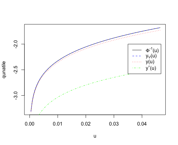 Figure 1
Peer Reviews
No public reviews on file for this paper yet. If you reviewed it on a platform where reviews are public (OpenReview, ICLR, NeurIPS, ICML), you can paste yours below so the community can read it here.
Videos
No videos yet. Explain this paper in a talk, walkthrough, or lecture? Add one.
Taxonomy
TopicsFinancial Risk and Volatility Modeling · Statistical Distribution Estimation and Applications · Probability and Risk Models
Quantile function expansion using regularly varying functions
Thomas Funga,111Corresponding Author. Honorary Associate, University of Sydney. Email address: [email protected] (Thomas Fung). and Eugene Senetab
a Department of Statistics, Macquarie University, NSW 2109, Australia
b School of Mathematics and Statistics, University of Sydney, NSW 2006, Australia
Abstract
We present a simple result that allows us to evaluate the asymptotic order of the remainder of a partial asymptotic expansion of the quantile function as or . This is focussed on important univariate distributions when has no simple closed form, with a view to assessing asymptotic rate of decay to zero of tail dependence in the context of bivariate copulas. The Introduction motivates the study in terms of the standard Normal. The Normal, Skew-Normal and Gamma are used as initial examples. Finally, we discuss approximation to the lower quantile of the Variance-Gamma and Skew-Slash distributions.
Keywords: Asymptotic expansion; asymptotic tail dependence; Quantile function; Regularly varying functions; Skew-Slash distribution; Variance-Gamma distribution.
1 Introduction
This paper is motivated by the need for a generally applicable procedure to study the asymptotic behaviour as of , and where the ’s are the inverse of continuous and strictly increasing cdf’s , , and a bivariate copula function respectively.
A random vector with marginal inverse distribution function , has coefficient of lower tail dependence if the limit exists, where
[TABLE]
If then X is said to be asymptotically independent in the lower tail. In this situation in particular the asymptotic rate of approach to the limit 0 of is an indication of the strength of asymptotic independence.
The classical case is the bivariate Normal with correlation coefficient as discussed in Embrechts, McNeil and Straumann (2011). It was shown in Fung and Seneta (2011) that if
[TABLE]
where , is the cdf of the standard Normal, and is a slowly varying function as , then
[TABLE]
Fung and Seneta (2011) also showed in their Theorem 3 that
[TABLE]
The proof within their Theorem 2 depended heavily on the very specific asymptotic relation as between the cdf and the corresponding standard Normal pdf .
We were unable to use in that paper, for this purpose, the expression for the quantile function of the standard Normal distribution
[TABLE]
given for example by Ledford and Tawn (1997) from a truncated expansion of , since we did not know the asymptotic order of the reminder . We were able to prove that as , but inasmuch as this asserts only that
[TABLE]
we can only be sure of the dominant term of a truncated asymptotic expansion, and this was inadequate to proceed from (1).
However our general result below, when applied to the standard Normal, gives
[TABLE]
Since
[TABLE]
as , from (1)
[TABLE]
where ;
[TABLE]
as , since , since as . Thus
[TABLE]
and the right hand side simplifies to the right hand side of (2).
In this note we present a simple result that allows us to evaluate the asymptotic order of the difference between and as or , where is the quantile function corresponding to a cumulative distribution function for important distributions where has no closed form, and is an asymptotic closed form expression. This is the general result which we discuss in Section 2. In Section 3, we will illustrate our results by considering the quantile function for the Generalised Gamma-type tail which has various commonly used distributions such as Normal, Skew-Normal, Gamma, Variance-Gamma and a Skew-Slash as special cases. Detailed extreme value structure of such distributions is important in a financial mathematics context. These individual examples will be discussed in Section 4.
2 Main Result
Our main result is summarised into the following Theorem.
Theorem 1**.**
Suppose that is a strictly positive continuous and strictly increasing cumulative distribution function (cdf) on , . Suppose further that some function as satisfies
[TABLE]
as , such that Suppose finally that with
[TABLE]
for some constant and function , , slowly varying at 0. If , is the inverse function of , then
[TABLE]
Proof.
We begin with the fact that
[TABLE]
Thus as and hence
[TABLE]
by the Uniform Convergence Theorem of slowly varying function of Seneta (1976, Theorem 1.1).
From (5), as . Finally,
[TABLE]
∎
Note that the formulation of the theorem requires, in the case only, that the function
The condition required in Theorem 1 is simply that the correction term in (4) is related to a regular varying function which is quite general and should apply to a wide range of distributions. The result in Theorem 1 not only ensures and will be asymptotically equivalent, it will also stipulate how accurate will be for .
We express as a corollary to Theorem 1 the corresponding result for the upper tail quantiles.
Corollary 1**.**
Suppose that is a strictly positive continuous and strictly increasing cumulative distribution function (cdf) on , . Suppose further that some function as satisfies
[TABLE]
as , such that If with
[TABLE]
for some constant and function , , slowly varying at 0. If is the inverse function of i.e. the upper tail quantile function then
[TABLE]
In the next section, we will illustrate our results by considering the quantile function corresponding to a cdf that has a Generalised Gamma-type tail behaviour.
3 Quantile for Generalised Gamma-type tail behaviour
3.1 Lower Tail
We are interested in approximation to the quantile function for the Generalised Gamma-type tail. We consider a cdf to have a Generalised Gamma-type (lower) tail behaviour if can be expressed as
[TABLE]
for some constants , , , and . Several distributions of current interest have such tails, and we discuss them as special cases in the next section.
Suppose that an approximation to the quantile function to be
[TABLE]
This can be obtained via the recursive method for an inverse function (see Chapter 2.4 of De Bruijn (1961) for instance) on . Then
[TABLE]
As , the behaviour of the quantile function is
[TABLE]
by Theorem 1.
We next expand to obtain an expansion for with an error term of appropriate lower order. After some algebra,
[TABLE]
As a result, when , becomes
[TABLE]
On the other hand, when , becomes
[TABLE]
3.2 Upper Tail
Similarly, a cdf is said to have a Generalised Gamma-type (upper) tail behaviour if can be expressed as
[TABLE]
for some constants , , , and , which would suggest the following approximation to the upper tail quantile function:
[TABLE]
Then by Corollary 1, the upper tail quantile function can be expressed as
[TABLE]
as .
4 Applications
In this section, we will illustrate our results with application to the Normal, Skew-Normal, Gamma, Variance-Gamma and Skew-Slash distributions.
4.1 Standard Normal
From Feller (1968) Chapter VII Lemma 2, the form of is
[TABLE]
If we compare this with (6), we have , , and . This means that the approximation becomes:
[TABLE]
and is the same as (3). As in this case we have , we can obtain the behaviour of the quantile function by using using (8) and (9) and get
[TABLE]
If we use only the dominating term of in (13) and so put
[TABLE]
then after some algebra we have
[TABLE]
As a result,
[TABLE]
by using Theorem 1. We can see that is a less accurate approximation to than and the expression for that it gives only improves on by giving the correct order of the difference .
We are aware that there exists a whole field of literature on finding an efficient and accurate approximation in the numerical sense for the Normal quantile functions, such as Abramowitz and Stegun (1964), Beasley and Springer (1977) to the more recent Voutier (2010). Soranzo and Epure (2014) provide a substantial bibliography on this subject. But that is not our focus and so our methodology will most likely be outperformed by the more sophisticated approximation in the literature. Take the approximation to the Normal quantile in Section 2.2.1 in Voutier (2010) for example which gives
[TABLE]
for where
[TABLE]
To see how the expansions perform against the approximations, we plot the standard Normal quantile function, denoted as , in R against , and and the results are shown in Fig. 1.
From Fig. 1, we can see that gives almost identical result to the built-in Normal quantile function in R and is better than our expansion . We also see that is an “order” worse than the other methods.
4.2 Skew-Normal
The quantile function of the Skew-Normal distribution is another example that is covered by our result. The distribution was first introduced by Azzalini (1985) and has developed into an extensive theory presented in a recent monograph by Azzalini and Capitanio (2014). A random variable is said to have a standard Skew-Normal distribution if its density function is
[TABLE]
where controls the skewness of the distribution. When , it reduces to the standard Normal as special case so we shall exclude the case of from our subsequent discussion. Using Lemma 2 of Capitanio (2010) or Azzalini and Capitanio (2014, pp. 52–53), we have
[TABLE]
This means if we compare (14) with (6), we have , , and when ; , , , when . This means that the approximation becomes:
[TABLE]
As in this case we have , we can obtain the behaviour of the quantile function by using (8) and (9) to get
[TABLE]
The expression (16) justifies the use of expression (15) above in Theorem 2 of Fung and Seneta (2016).
4.3 Gamma
Using (12), one can also determine the accuracy of the gamma-like upper tail. Suppose that and let its pdf be
[TABLE]
Then
[TABLE]
as . This means that if we compare (17) with (10), we have , , and . By using (11) an approximation to the upper quantile function when would be
[TABLE]
As in this case we have again, we have for the upper quantile function
[TABLE]
as by using (12).
In Section 4 of Fung and Seneta (2011), via their Theorem 1, the authors obtained with
4.4 Variance-Gamma and Skew-Slash
Finally, we propose an approximation to the lower tail quantile function of the Variance-Gamma (VG) and a Skew-Slash distribution, as they can have similar tail structure. A random variable is said to have a skew VG distribution introduced in Madan, Carr and Chang (1998) and further studied in Schoutens (2003), Seneta (2004) and Tjetjep and Seneta (2006), if X is defined by a Normal variance-mean mixture as , where and . The distribution of is with such that . When and , from Schoutens (2003), we have
[TABLE]
as , where is defined by the above.. By comparing with (6), is defined as above, , and which in turn would suggest the following approximation to the lower quantile function:
[TABLE]
as by using (7). We can then obtain the behaviour of the quantile function as
[TABLE]
A Skew-Slash distribution on the other hand was first proposed in multivariate form in Arslan (2008) and further studied in Ling and Peng (2015). A random variable is said to have a Skew-Slash distribution if is defined by a Normal variance-mean mixture as , where , and . The distribution of is Beta); that is, its pdf is: Here we only consider the case of so that the tail behaviour is similar to that of the Variance-Gamma in (18). When , and , from Ling and Peng (2015, Lemma 2.1 and equation (11)), we have
[TABLE]
as . By comparing this with (6), we have , , , and , which in turn suggests the following approximation to the lower quantile function:
[TABLE]
as by using (7). Ling and Peng (2015, Lemma 3.1, equation (3)) use the fact that , with . We can obtain the behaviour of the quantile function as
[TABLE]
as by using (8) and (9) once again.
Acknowledgements
The authors thank the referee for a careful reading of the original version, and a list of suggestions which have resulted in a much improved paper.
The reference list from the paper itself. Each links out to its DOI / PubMed record.
- 1Abramowitz and Stegun (1964) Abramowitz, M. and Stegun, I.E. (ed.), Handbook of Mathematical Functions With Formulas, Graphs and Mathematical Tables. National Bureau of Standards, Washington.
- 2Arslan (2008) Arslan, O. (2008) An alternative multivariate skew-slash distribution. Statistics and Probability Letters 78:2756–2761.
- 3Azzalini (1985) Azzalini, A. (1985) A class of distributions which includes the normal ones. Scand. J. Statist. 12:171–178.
- 4Azzalini and Capitanio (2014) Azzalini, A. and Capitanio, A. (2014) The Skew-Normal and Related Families. IMS Monographs. Cambridge University Press, Cambridge.
- 5Beasley and Springer (1977) Beasley, J. D. and Springer S. G. (1977). The percentage points of the Normal Distribution, Applied Statistics 26, 118–121.
- 6Capitanio (2010) Capitanio, A. (2010) On the approximation of the tail probability of the scalar skew-normal distribution. Metron 68:299–308.
- 7De Bruijn (1961) De Bruijn, N.G. (1961) Asymptotic Methods in Analysis. 2nd Ed. North-Holland Publishing Co., Amsterdam.
- 8Embrechts, Mc Neil and Straumann (2011) Embrechts, P., Mc Neil, A. and Straumann, D. (2001). Correlation and dependency in risk management: properties and pitfalls. In, Dempster, M. and Moffatt, H., eds. Risk Management: Value at Risk and Beyond . Cambridge University Press, Cambridge, pp.176-223.