Discovery of statistical equivalence classes using computer algebra
Christiane G\"orgen, Anna Bigatti, Eva Riccomagno, Jim Q. Smith

TL;DR
This paper introduces a novel algorithm leveraging computer algebra to identify all nested representations of interpolating polynomials in discrete statistical models, enabling efficient discovery of equivalence classes of event trees.
Contribution
It presents a new method using primary decomposition of monomial ideals to compute all nested representations of interpolating polynomials in statistical models.
Findings
Identifies all nested representations of a polynomial in polynomial time.
Analyzes the equivalence class of a real-world staged tree model.
Demonstrates the method on a dataset fitting scenario.
Abstract
Discrete statistical models supported on labelled event trees can be specified using so-called interpolating polynomials which are generalizations of generating functions. These admit a nested representation. A new algorithm exploits the primary decomposition of monomial ideals associated with an interpolating polynomial to quickly compute all nested representations of that polynomial. It hereby determines an important subclass of all trees representing the same statistical model. To illustrate this method we analyze the full polynomial equivalence class of a staged tree representing the best fitting model inferred from a real-world dataset.
Click any figure to enlarge with its caption.
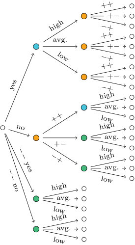 Figure 1
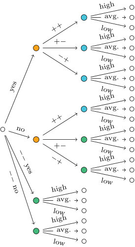 Figure 2
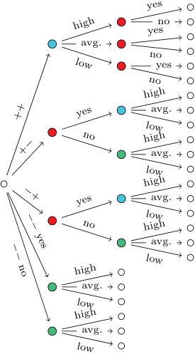 Figure 3
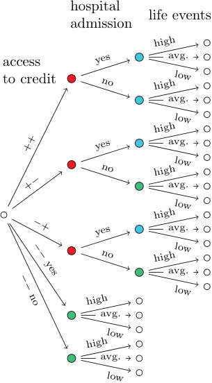 Figure 4
 Figure 5
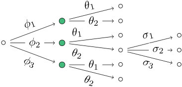 Figure 6
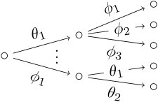 Figure 7
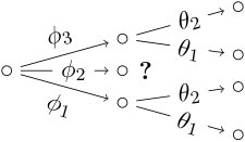 Figure 8
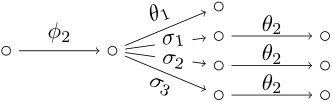 Figure 9
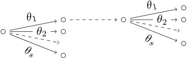 Figure 10
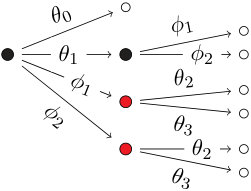 Figure 11
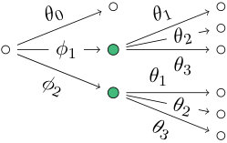 Figure 12
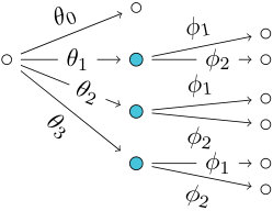 Figure 13
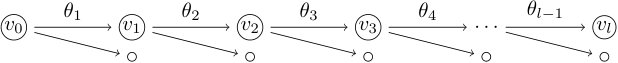 Figure 14
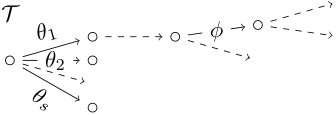 Figure 15
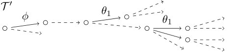 Figure 16
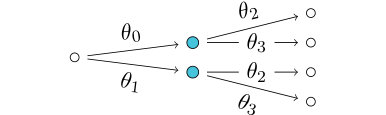 Figure 17
 Figure 18
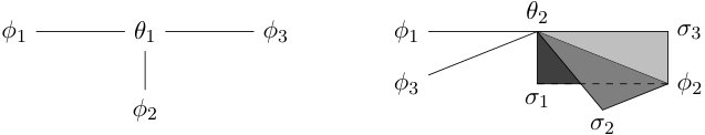 Figure 19
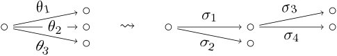 Figure 20
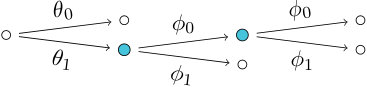 Figure 21
| stage colour | label | interpretation |
|---|---|---|
| access to credit: | ||
| hospital admission: yes or no | ||
| number of life events: high, average or low | ||
| number of life events: high, average or low | ||
| access to credit: |
Peer Reviews
No public reviews on file for this paper yet. If you reviewed it on a platform where reviews are public (OpenReview, ICLR, NeurIPS, ICML), you can paste yours below so the community can read it here.
Videos
No videos yet. Explain this paper in a talk, walkthrough, or lecture? Add one.
Taxonomy
TopicsTopological and Geometric Data Analysis · Gene Regulatory Network Analysis · Bayesian Modeling and Causal Inference
Discovery of statistical equivalence classes using computer algebra
Christiane Görgen, Anna Bigatti, Eva Riccomagno and Jim Q. Smith
Abstract
Discrete statistical models supported on labelled event trees can be specified using so-called interpolating polynomials which are generalizations of generating functions. These admit a nested representation. A new algorithm exploits the primary decomposition of monomial ideals associated with an interpolating polynomial to quickly compute all nested representations of that polynomial. It hereby determines an important subclass of all trees representing the same statistical model. To illustrate this method we analyze the full polynomial equivalence class of a staged tree representing the best fitting model inferred from a real-world dataset.
Keywords Graphical Models; Staged Tree Models; Computer Algebra; Ideal Decomposition; Algebraic Statistics.
1 Introduction
Families of finite and discrete multivariate models have been extensively studied, including many different classes of graphical models [19, 2]. Because these families of probability distributions can often be expressed as polynomials – or collections of vectors of polynomials – this has spawned a deep study of their algebraic properties [23, 21, 10]. These can then be further exploited using the discipline of computational commutative algebra and computer algebra software such as CoCoA [1] which has proved to be a powerful though somewhat neglected tool of analysis.
In this paper, we demonstrate how certain computer algebra techniques – especially the primary decomposition of ideals – can be routinely applied to the study of various finite discrete models. Throughout we pay particular attention to an important class of graphical models based on probability trees and called staged trees or chain event graph models [27]. These contain the familiar class of discrete (and context-specific) Bayesian networks as a special case. In particular, [16] gave a mathematical way of determining the statistical equivalence classes of staged tree models but did not give algorithms to actually find these. Here we use computer algebra in a novel way to systematically find a staged tree representation of a given family – if it indeed exists – and to uncover statistically equivalent staged trees in an elegant, systematic and useful way. This is an extensions of the techniques developed by [2] and others to determine Markov-equivalence classes of Bayesian networks where, instead of algebra, graph theory was used as a main tool.
So our methodology supports a new analysis of a very general but fairly recent statistical model class in a novel algebraic way and serves as an illustration of how more generally computer algebra can be a useful tool not only to the study of conventional classes of graphical model but other families of statistical model as well.
2 Staged trees and interpolating polynomials
2.1 Labeled event trees and staged trees
In this work we will exclusively consider graphs which are trees, so those which are connected and without cycles. We first review the theory of staged trees which represent interesting and very general discrete models in statistics [27].
Definition 1** (Labeled event trees).**
Let be a finite directed rooted tree with vertex set and edge set . We denote the root vertex of by .
The tree is called an event tree if every vertex has either no, two or more than two emanating edges. For , let denote the set of the edges emanating from . The pair is called a floret.
Let be a non-empty set of symbol/labels and let a function be such that for any floret the labels in are all distinct. We call the floret labels of and denote this set by . The pair of graph and function is called a labeled event tree. When takes values in and , is called a probability tree111We should say more precisely: when the symbols are evaluated in for all . .
For , the labeled subtree rooted in is , where is the largest subtree of rooted in , and is the restriction of to the edges in .
For any leaf , so for any vertex with no emanating edges, we trivially have that , and hence .
labeled event trees are well-known objects in probability theory and decision theory where they are used to depict discrete unfoldings of events. The labels on edges of a probability tree then correspond to transition probabilities from one vertex to the next and all edge probabilities belonging to the same floret sum to unity. See [25] for the use of probability trees in probability theory and causal inference, and see for instance [24] for how such a tree representation can be used in computational statistics.
In this paper, we generally do not require the labels on a labeled event tree to be probabilities.
Definition 2** (Staged trees).**
A labeled event tree , with , is called a staged tree if for every pair of vertices their floret labels are either equal or disjoint, or . A stage is a set of vertices with the same floret labels.
In illustrations of staged trees, all vertices in the same stage are usually assigned a common color: compare Fig. 1. Staged trees were first defined as an intermediate step to building chain event graphs as graphical representations for certain discrete statistical models [26]. Every chain event graph is uniquely associated to a staged tree and vice versa. In this way, the graphical redundancy of staged trees can be avoided, and elegant conjugate analyzes can be applied to staged tree models [28, 12, 3, 6]. In particular, every discrete and context-specific Bayesian network can alternatively be represented by a staged tree where stages indicate equalities of conditional probability vectors. We give examples of this later in the text.
For the development in this paper it is important to observe that staged trees with labels evaluated as probabilities are always also probability trees. This is however not the case for all labeled event trees because sum-to- conditions imposed on florets can be contradictory. See also Examples 2 and 9 below.
Example 1** (Saturated trees).**
A saturated tree is a labeled event tree where all edges have distinct labels. So this is a staged tree where all floret labels are disjoint, or alternatively with every stage containing exactly one vertex. In the development below, saturated trees are graphical representations of saturated statistical models.
Example 2**.**
Figure 1a shows a staged tree where all blue-coloured vertices are in the same stage. Figure 1b depicts a staged tree where the two green vertices are in the same stage. Figure 1c show a labeled event tree which is not staged because the floret labels of the two black vertices are neither equal nor disjoint.
2.2 Network polynomials and interpolating polynomials
We next define a polynomial associated to a labeled event tree which is the key tool used in this paper: see also [16].
Definition 3** (Network and interpolating polynomials).**
Let be a labeled event tree and let denote the set of root-to-leaf paths in . For let be the set of edges of . We call the products of the labels along a root-to-leaf path, , atomic monomials.
Given a real-valued function , we define the network polynomial of and , the linear combination of the atomic monomials with coefficients given by , as:
[TABLE]
with the particular case if has no edges. The interpolating polynomial is the network polynomial with all equal to one, and we write .
Remark 1*.*
A network polynomial is a polynomial in the ring of polynomials with real coefficients and whose indeterminates are the labels in . An interpolating polynomial is a polynomial with positive integer coefficients by construction. For these we write .
Example 3**.**
When is a probability tree, every atomic monomial is the product of transition probabilities along a root-to-leaf path and thus the probability of an atomic event (or atom). Often the function is an indicator function of an event . In this case, Eq. 1 is a polynomial representation of the finite-additivity property of probabilities for , so .
Interpolating polynomials have been used successfully to classify equivalence classes of staged trees which make the same distributional assumptions [16], as outlined in Section 3 below. They have further been used as a tool for calculating marginal and conditional probabilities in Bayesian networks and staged trees, using differentiation operations [8, 15].
In Theorem 1 and Proposition 1 for the purposes of this paper we now present two central results on interpolating polynomials. These results are given here in a reformulated, recursive form and very different from their original development [16, Proposition 1]. This refinement is necessary because the new proofs we give are constructive and, most importantly, transparently illustrate the mechanisms needed for our later algorithmic implementation.
Theorem 1**.**
Let be an event tree and for define
[TABLE]
Then the interpolating polynomial of is equal to where is the root of .
Proof.
We prove the claim by induction on the depth of the tree, i.e. the number of edges in the longest root-to-leaf path. If has depth then and . If has depth then
[TABLE]
Furthermore,
[TABLE]
and by the inductive hypothesis because the subtrees all have lower depths than . ∎
Example 4**.**
The two staged trees and in Fig. 2 have the same interpolating polynomial, so the same sum of atomic monomials:
[TABLE]
Here, the functions and assign the same labels to different edges in the graphs and . Following the recursive construction in Theorem 1, we can then write this polynomial in terms of the interpolating polynomials of subtrees:
[TABLE]
where and ; or alternatively
[TABLE]
where , and .
Example 4 shows that the distributive property of multiplication over addition is at the core of our work. The following corollary will be useful for studying staged trees with square-free atomic monomials: compare also Proposition 3 below.
Corollary 1**.**
Let be a labeled event tree and let be its interpolating polynomial. Then we can write
[TABLE]
Moreover, if the root labels are not repeated, i.e. for all , then no label in appears in any subtree-interpolating polynomial .
Proof.
The proof is a trivial consequence of the construction of the polynomial in Theorem 1 above. ∎
Example 5**.**
Consider again the two staged trees in Example 4. Their interpolating polynomial admits two different representations in terms of a linear combination as in Corollary 1, namely the ones in Eq. 6 and Eq. 7. We can see here explicitly how the polynomials above depend on the variables in subtrees of and . In particular, both sets and provide potential root-floret labels of a corresponding tree representation.
2.3 Polynomials with a nested representation
We know now that we can straightforwardly read an interpolating polynomial, and in particular a recursive representation of that polynomial, from a labeled event tree. In this section and in Section 5 we consider the inverse problem: given a polynomial in distributed form can we tell whether it is the interpolating polynomial of a labeled event tree? In order to answer this question first observe that the polynomials defined below admit a special structured representation and can be used as a surrogate for a labeled event tree as shown in Proposition 1.
Definition 4** (Nested representation).**
Let be a polynomial with positive integer coefficients. We say that admits a nested representation if or if it can be written as where is such that and, for each , the polynomial admits a nested representation.
Remark 2*.*
The recursion in Definition 4 is finite because , for by construction polynomials with nested representations have positive coefficients.
The polynomial in Theorem 1 is written in nested representation by construction. In this sense Proposition 1 below is the inverse result of Theorem 1, and a polynomial admits a nested representation if and only if it is the interpolating polynomial of a labeled event tree.
Proposition 1**.**
If admits a nested representation then there exists a labeled event tree such that .
Proof.
We prove the claim by induction on the degree of . If then and therefore where is formed by a single vertex with no edges and no labels.
If then and therefore by Remark 2 and by induction for some tree labeled over . For all let be the root of . Then a tree with interpolating polynomial can be constructed by taking a new vertex assigned as the root of and defining the edges of the root floret to be . Then . ∎
The result above implies in particular that if is a polynomial with nested representation then the root labels of a tree with interpolating polynomial are given by .
Example 6**.**
The nested representations of the two event trees and in Fig. 2 are
[TABLE]
as in Examples 4 and 5. These nestings are in one-to-one correspondence with the depicted trees, just as stated in Proposition 1.
Example 7**.**
Let and consider the polynomial . Then has nested representation corresponding to a labeled event tree which is not staged.
Example 8**.**
Let and consider the polynomial
[TABLE]
Then admits three different nested representations:
[TABLE]
In particular, Eq. 11a corresponds to the staged tree in Fig. 1a and Eq. 11b to the staged tree in Fig. 1b. In Section 4 we show that there are no other staged trees with interpolating polynomial . The third nested representation Eq. 11c corresponds to the labeled event tree in Fig. 1c which is not staged.
In the above examples, a given polynomial can admit several different nested representations. By the result below, this is not always the case.
Proposition 2** (Saturated trees).**
For a saturated tree , the interpolating polynomial has a unique nested representation.
Proof.
Let be a labeled event tree, not necessarily saturated nor staged, with interpolating polynomial . We prove that , i.e. is indeed the saturated tree .
Let be the set of power-products (or monomials) in , and for a label indicate the set of all multiples of that label with .
Let and , respectively, be the set of root-floret labels of and , so in Definition 1 w.r.t. and . We first prove that . For any the power-products in , corresponding to the root-to-leaf paths originating from the root-edge in which is labeled , are not multiples of any for because is saturated. Thus, if and then the power-products in could not correspond to root-to-leaf paths in .
It follows that if then there must be a label with . Since is saturated, is the label of only one edge in , and this edge is, say, in the subtree starting from the root edge labeled . In terms of the power-products, this implies that . Hence, in all root-to-leaf paths originating from the root edge labeled by must have an edge labeled : see the figure below.
Now consider the root-to-leaf path in where appears at greatest depth, i.e. with the longest path from the root vertex. The floret containing must have at least another edge so the paths through this other edge have at greater depth. But this is a contradiction. Hence .
The subtrees of rooted in the children of its root are again saturated trees, and their interpolating polynomials are for and have disjoint sets of labels because is saturated. Therefore we can repeat the reasoning above on these subtrees and their interpolating polynomials. We conclude in a finite number of steps that . ∎
Thus when reading an interpolating polynomial from a tree, instead of summing atomic monomials as in Definition 3 we can directly use the tree graph to infer a bracketed, nested representation of that polynomial. This representation is in one-to-one correspondence with the labeled graph itself, so the original representation can be easily recovered. Similarly, once we are given any polynomial in distributed form and this polynomial admits such a nested bracketing then we can always find a corresponding tree representation. These insights open the door to replace graphical representations of statistical models by polynomial representations, and hence enable us to employ computer algebra in their study. We will show how this can be done in the next section.
3 Polynomial and statistical equivalence
Computer algebra is often used to study polynomials that arise naturally in statistical inference. For instance, context-specific Bayesian networks, staged trees and chain event graphs are all parametric statistical models whose probability mass function is of monomial form: for every atom in an underlying sample space where . This monomial can then be thought of as for instance a product of potentials [19] or simply a product of edge probabilities in a staged tree with root-to-leaf paths as atoms. So the network and interpolating polynomials as in Definition 3 can be defined for all parametric models admitting a general monomial parametrization as given above [20]. We can then apply the theory above to these models and employ computer algebra techniques in their study. In particular, often very different parametrizations can give rise to the same model and the interpolating polynomial can help to determine these.
Definition 5** (Polynomial and statistical equivalence).**
Two staged trees and with the same label set are called polynomially equivalent if their interpolating polynomials are equal.
Two staged trees and with possibly different label sets, say and , are called statistically equivalent if there is a bijection which identifies their root-to-leaf paths and for any evaluation function on , namely extended to as , there exists an evaluation on , , such that for all .
By definition, two staged trees whose labels are evaluated as probabilities are statistically equivalent if and only if they represent the same statistical model.
Since the interpolating polynomials of polynomially equivalent trees are equal, they are the sum of the same atomic monomials. Therefore there is a bijection between the root-to-leaf paths of polynomially equivalent trees. This implies that polynomially equivalent trees are also statistically equivalent. For instance, the trees from Examples 5 and 6 are polynomially, and so statistically equivalent. In particular, the interpolating polynomial is sufficient to determine a probability distribution up to a permutation of the values it takes across an underlying sample space.
From Proposition 1, the class of polynomially equivalent trees is fully described by all nested representations of the interpolating polynomial. Indeed, when reordering the terms of a nested representation as in Fig. 2, the atomic monomials of the underlying tree do not change. So if we are given the interpolating polynomial of a staged tree and we can find all its possible nested representations then we have automatically found all of its polynomially equivalent tree representations – and often a large subclass of the whole statistical equivalence class. For example, in the case of decomposable Bayesian networks the equivalence class of a polynomial given in clique parametrization contains the Markov-equivalence class [14].
Polynomially equivalent trees can be thought of as those having the same parametrization. However this parametrization is often read in a different non-commutative way for different graphical representation in that class. For instance, the staged trees in Examples 5 and 6 have the same atomic monomials belonging to identified atoms but in and in for identified atoms and . Analogous instances of this phenomenon occur in the class of decomposable Bayesian networks where a model parametrization can be given by potentials on cliques which are renormalized across different graphical representations of the same model.
Statistically equivalent trees however can be thought of as reparametrizations of each other, very much like in Bayesian networks where a parametrization can either be based on parent relations between single nodes in a graph or alternatively on clique margins. See also Example 12.
Example 9**.**
Polynomially equivalent trees can often be described by a variety of different graphs. For instance, the polynomial has at least three different labeled trees associated: see Fig. 1 and Example 8.
The two trees in Figs. 1a and 1b are polynomially equivalent representations of the same model on seven atoms. The tree in Fig. 1c is not because it is not a staged tree. In particular, this tree is not a probability tree because sum-to- conditions imposed on its florets would be contradictory.
Example 10** (Maximal representations).**
For any labeled event tree there exists a statistical equivalent binary labeled event tree whose graph is such that for all . This can be thought of as a maximal representation within the class of statistically equivalent trees. We can easily obtain a binary tree by splitting up each floret with strictly more than two edges as shown in Fig. 3.
In particular, for a floret in a probability tree labeled by , we would obtain new labels which are renormalizations of the original parameters such that sum-to- conditions hold, and , while retaining the distribution over the three depicted atoms, so , , and .
Example 11** (Minimal representations).**
In the polynomial equivalence class of a saturated tree there is exactly one member, namely the tree itself. This is because, by Proposition 2, for saturated trees the nested representation of an interpolating polynomial is unique. The statistical equivalence class of a saturated tree however is much bigger. This is a consequence of Example 10 above. In particular, for every saturated tree there is a unique minimal graphical representation given by a single floret whose labels are the atomic monomials (or joint probabilities) and whose number of edges coincides with the number of root-to-leaf paths in any equivalent representation.
In the development in this paper we mainly focus on a parametric characterization of staged tree and other statistical models. This naturally links in with an alternative implicit characterization which is well known in algebraic statistics. For instance, a polynomial representation of a Bayesian network involving exclusively the joint probabilities – i.e. the values of the associated probability mass function as varies in the sample space – can be derived from the equalities using ring operations. The algebraic theory behind this is called elimination theory [18] of which Gaussian elimination for solving systems of linear equations is a simple example. The representation of a Bayesian network as such a set of polynomials is an algebraic structure called a toric ideal and has great importance in algebraic statistics: see e.g. [23, 13, 10].
Notably, this alternative characterization can also be used to describe statistical equivalence – though in a less constructive way than the method we present here and without immediate links to a graphical representation of a model.
Example 12**.**
The labeled event tree in Fig. 4a is a staged tree on four atoms with labels . The equalities holding for the four atomic monomials
[TABLE]
imply the equality . This parametrization of the model in Fig. 4a is not to be confused with the minimal representation of the saturated model on four atoms in Fig. 4b.
An interpretation of this equation is as follows. Assume two binary random variables are such that
[TABLE]
Then is an instance of a fundamental relationship in algebraic statistics for representing conditional independence of discrete random variables: see e.g. [23, Section 6.10] and [10, Proposition 3.1.4]. In this specific case the equality implies that and are independent.
4 From polynomials to trees: finding the nested
representations
4.1 Potential root-floret labels and square-free monomials
Building on the results above we can now use methods from commutative algebra to compute all the staged trees with a given interpolating polynomial and so to compute a complete polynomial equivalence class. The two key notions we use to build an algorithm which determines these classes are those of a monomial ideal and of its primary decomposition which, for square-free monomials, coincides with the prime decomposition. These notions are recalled in the appendix.
The key of the proposed algorithm is Theorem 2 below. This states in algebraic terms that for any tree each monomial in is divisible by some label in the set of the floret labels belonging to the root of , and that is minimal (with respect to inclusion) with this property.
Theorem 2**.**
Let be a staged tree. The monomial ideal generated by the root-floret labels is a minimal prime of the ideal generated by the support of .
Proof.
Let be the set of root-floret labels. Then each power-product in is a multiple of some label in . Because it is generated by indeterminates, is a prime ideal containing all power-products in . Suppose, by contradiction, that is not minimal. Then there exists with containing all power-products in . Without loss of generality let . Now, each root-to-leaf path starting with the root edge labeled has an associated atomic monomial , . Therefore for some . As is staged, this implies that the whole root floret must appear again in the subtree: see the illustration below.
Next consider the subtree containing the repeated root-floret labels at a minimum depth and repeat the reasoning above: each root-to-leaf path containing the two edges labeled corresponds to an atom and is therefore a multiple of some label in . Then the whole root floret is repeated again deeper in the subtree, producing some atom divisible by . Since this reasoning can be repeated a finite number of times, we have the contradiction that there is an atomic monomial divisible by a power of and by no label in . Therefore is minimal. ∎
Example 13**.**
The interpolating polynomial in Example 4 has support
[TABLE]
The primary decomposition of the corresponding square-free monomial ideal is
[TABLE]
Therefore, by Theorem 2, there are three different sets of possible root labels for a staged tree with interpolating polynomial . We show in Example 15 below that the polynomial equivalence class of is given by just two trees.
Example 14**.**
Consider the interpolating polynomial . The minimal prime decomposition of is given by two sets, namely and . The first one leads to the tree in Fig. 5. It can be shown by exhaustive search that the second does not give the labels of a root floret in a labeled event tree.
The key assumption in Theorem 2 is that the input tree is staged, otherwise the result need not be true.
This theorem is central to the algorithm we present in the following section because it shows that instead of searching for root-floret labels among all subsets of labels , the search can be limited to those subsets which are the generators of the minimal primes of . If has elements, their number is bounded above by whereas the number of the subsets of is . So considering all possible subsets of , and having to repeat this recursively, may lead to a combinatorial explosion of cases to analyze. As a consequence, Theorem 2 gives a drastic reduction of the set of candidate root-floret labels.
Staged trees whose interpolating polynomials are sums of square-free power-products are interesting cases both from an algebraic viewpoint and for their interpretation in statistical inference. For instance, if all power-products in are square-free then the proof of Theorem 2 can be shortened obtaining the contradiction by Proposition 3 directly. In terms of staged tree models, this condition implies that if a unit passes through a vertex in a given stage it cannot subsequently pass through another vertex in the same stage. By making this requirement we can avoid various complex ambiguities associated with exactly how we relate a sample distribution to a polynomial family. Although less useful in modeling time series, in most cross-sectional statistical models this constraint will almost always apply.
The restriction to polynomials with square-free support enables us to prove the second and third central result for our algorithmic implementation.
Proposition 3** (Root-floret labels).**
Let be a staged tree whose interpolating polynomial is a sum of square-free power-products. Then no label in appears in any subtree-polynomial .
Proof.
Because is a staged tree we have or for all by Definition 3. By contradiction, suppose there is a subtree containing a floret with labels . Let be the label of the edge for some . Then there is a root-to-leaf path with at least two edges labeled : see also the illustration in the proof of Theorem 2. Hence there is a multiple of in . This is a contradiction because is a sum of square-free power-products. So there is no subtree containing a floret with labels . The claim follows from Corollary 1. ∎
Corollary 2**.**
Let be a staged tree whose interpolating polynomial is a sum of square-free power-products. Then all coefficients in are equal to 1.
Proof.
The claim follows from Proposition 3 and its recursive application to subtrees of . ∎
So when searching for staged trees using square-free interpolating polynomials, coefficients might be ignored. This is not true for labeled event trees by Example 7. In Section 4.3 we will see that this result will allow the application of the algorithm in Section 4.2 to network polynomials of staged trees.
4.2 The algorithm StagedTrees
Given a polynomial whose power-products are square-free and with coefficients all equal to one, there is an obvious algorithm which determines all its nested representations, and in particular all staged trees for which is the interpolating polynomial. This algorithm is here called StagedTrees and is given in pseudo-code in Algorithm 1. Following the notation in Definition 4, the proposed algorithm searches over subsets of the indeterminates appearing in and recursively checks whether it is possible to construct the polynomials for . The choices of are hereby constrained to the minimal primes of the monomial ideal associated to as determined by Theorem 2. This algorithm works even when it is not known a priori whether or not is the interpolating polynomial of a staged tree. Since the support of is finite it is clear that the recursion terminates. The function StagedTrees is part of the CoCoA distribution from version 5.1.6 (http://cocoa.dima.unige.it/download/CoCoAManual/html/cmdStagedTrees.html).
The base steps of the recursion in Algorithm 1 are given by the simplest trees: a single vertex tree for (Step 2), or a floret without subtrees for (Step 4) with at least two edges (Step 3). Compare also the recursive description in Theorem 1. In Step 5, Theorem 2 is applied to determine the candidate root-florets . The main loop in Step 6 considers each one at a time, and determines all the staged trees having root floret , .
In the main loop, Step 6.2 checks if the subsets defined in Step 6.1 give a partition for which is a necessary condition from Proposition 3: since is a minimal prime for it follows that . Therefore only disjointness needs to be verified. Then the inner loop in Step 6.3, with its sub-steps, considers one at a time each , and determines (if possible) all the subtrees emanating from the second vertex of the edge labeled . In particular, Step 6.3.1 stops the search for if there is a single emanating edge and therefore by definition not an event tree. Step 6.3.3 makes the recursive call on (defined in Step 6.3.2) to determine the set of all possible subtrees from . If is empty then Step 6.3.4 stops the search for .
Concluding the main loop, Step 6.4 is reached if for each edge having a label in there is at least one subtree. Then the floret labeled by together with all combinations of its subtrees make a set of event trees, with root-floret labels , whose interpolating polynomial is the sum of the monomials in . At this point Step 6.5 discards those which are not staged. In particular the subtrees are staged, and compatibility of stages across the subtrees is checked here, in the obvious way. Finally, Step 6.6 stores them in .
Example 15**.**
We illustrate the working of the StagedTrees algorithm on Example 4. From Example 13 we can consider only three sets of potential root-floret labels of staged trees with interpolating polynomial given in Eq. 5. These are:
[TABLE]
The first set cannot be a floret-label set because , see Step 6.2 in the algorithm. Indeed the two sets
[TABLE]
show that, if were a floret-label set, then the tree would include a structure such as in Fig. 6a which cannot be part of a staged tree: see also Corollary 1 and Proposition 3. Above we have used the convention that the product of a single label with a set of labels is defined as the set of all elementwise products.
With in the first step of the algorithm we have
[TABLE]
The algorithm calls recursively on the sets and but stops immediately (Step 4 in the algorithm) as summarized in Fig. 6b. For the middle branch we need to continue the recursion by working on . The monomial ideal generated by has the following primary decomposition
[TABLE]
Taking gives the tree in Fig. 2b while leads to the situation in Fig. 6c which does not correspond to an event tree. In conclusion, gives the tree in Fig. 2b only. The result of the algorithm starting from is analogous and leads to the tree in Fig. 2a.
4.3 Discussion of the algorithm
It was shown in [16] that the application of two graphical operators called the “swap” and “resize” on a staged tree could be used to traverse a statistical equivalence class. However these authors did not provide an implementation of their graphical methods in algebraic or computational terms. So Algorithm 1 fills that gap and enables us to determine the full polynomial equivalence class of a given staged tree. We hereby focus on staged as opposed to labeled event trees because these can always be interpreted as representations of statistical models as in Sections 2 and 3. Of course our new algorithm can be easily adapted to discover more general representations. We will now discuss some of the properties of this algorithm.
First, the StagedTrees algorithm can be modified to work on non-square-free power-products. For this purpose Step 6.2 must be disabled and all the possible partitions of need to be checked, making the algorithm more expensive. For example, the only minimal prime for the ideal is which leads to two partitions , and . Calling the algorithm on the first partition gives no answer because it leads to a tree which is not an event tree, whereas the second gives the original nested representation. Moreover, in this partitioning one also needs to keep track of the coefficients: as illustrated by the nested representation .
Second, so far we often emphasized the use of the interpolating polynomial as opposed to the network polynomial in Definition 3. This was to highlight the structure of the tree, as opposed to the real values associated its root-to-leaf paths: compare also Definition 5. However, if is the network polynomial associated to a staged tree and its power-products are square-free, from Proposition 3 it follows that the root-to-leaf paths are labeled by distinct monomials. This means that in the network polynomial the coefficients are kept distinct. In conclusion, all staged trees with a given network polynomial are found by the algorithm StagedTrees applied to . Afterwards the coefficients can be associated to the corresponding root-to-leaf paths.
Third, thanks to the reduction to minimal primes, the algorithm is very fast also for real-world settings. In Section 7 we will apply StagedTrees to discover the polynomial equivalence class of a staged tree describing a real problem with 24 atomic events. This computation takes much less than a second on a laptop with a 2.4 GHz Intel Core 2 Duo processor. Similarly, it takes 2.3 seconds to compute the 576 staged trees sharing the interpolating polynomial representing four independent binary random variables: compare Fig. 4a. Computing the polynomial equivalence class of four independent random variables taking three levels each takes significantly longer at 12:23min but produces 55,296 different staged trees, each having 81 atoms. Naturally, the more stage structure there is present the more different polynomially equivalent representations are possible, so the latter two are somewhat extreme cases. On medium-sized real-world applications like the one presented below our computations are very fast. So this algorithm allows us to systematically enumerate and analyze staged trees of the same order or even bigger than the study we will consider.
Fourth, every Bayesian network, context-specific Bayesian network [4] and object-oriented Bayesian network [17] can be represented by a staged tree where inner vertices correspond to conditional random variables and the emanating edges correspond to the different states of these variables. Then two vertices are in the same stage if and only if the corresponding rows of conditional probability tables are identified. For instance, the independence model of two binary random variables can be represented by the staged tree depicted in Fig. 4a. The complete Bayesian network on two binary random variables can be represented by the staged tree in Fig. 4b. However, staged trees allow for much less symmetric – and hence more general – modeling assumptions. In particular, they do not rely on an underlying product-space structure but can express relationships directly in terms of events. So this class of models is much larger than the Bayesian network class and as a consequence the StagedTrees algorithm can be optimized to traverse this wider class as well as the class of Bayesian networks.
So the methodology we developed for the StagedTrees algorithm will serve as a springboard for really fast algorithms to analyze equivalence classes of staged trees and in the future causal discovery algorithms over this class: see also Section 7. We illustrate below that these computer algebra analysis enable us to obtain further insights about the properties of the underlying class of statistical models.
5 Additional properties of interpolating polynomials
A natural question to ask is whether or not a given polynomial can be seen to be the interpolating polynomial of an event tree without having to construct a nested representation first. The following proposition gives some necessary conditions for a polynomial to be an interpolating polynomial of a labeled event tree.
Recall that for a power-product , the degree is the sum of the exponents, , and for a polynomial the degree is .
Proposition 4**.**
Let be a polynomial with square-free support, i.e. for all and some . If there exists a labeled event tree such that is its interpolating polynomial then the following conditions hold:
If then and , and . 2. 2.
The frequency with which each root label appears in the monomials , , is greater than the degree of the monomials in which they appear. 3. 3.
If the degree of is equal to the degree of , then there exists with with the same degree as and the degree of the greatest common divisor of and is equal to the degree of minus one. 4. 4.
No power-product in the support of can be a proper multiple of another.
Proof.
The root floret of a labeled event tree with at least one edge has at least two edges with distinct labels, thus . We prove the claim by induction on the number of florets in a labeled event tree. Let be the set of edges and the set of leaves of the tree. If a tree is formed by a single vertex then and . Therefore . By induction suppose that for the tree . Consider the tree obtained by adding to a leaf in a floret with edges. Because , thus and hence and . As a result, . We conclude by noticing that and . 2. 2.
Consider Fig. 7. In labeled event trees, an atomic monomial of degree is associated to a root-to-leaf path of length . This path has one bifurcation at every vertex, so is embedded in a graph with at least distinct root-to-leaf paths. So every root-label occurs in monomials of maximal degree and there are at least of those. 3. 3.
Because for all , every leaf-floret has two edges. There are hence at least two monomials of the same maximal degree, namely those belonging to the longest paths in the tree: these are equal until they split at a leaf-floret.
Let and in be multiples of each other, written as . They are atomic monomials of two root-to-leaf paths, and , which are not empty if is not trivial. Let be the root edge labeled , the first edge in . Then starts with the same edge: otherwise , and for Proposition 3. Therefore we can repeat the reasoning on and in the subtree . After a finite number of steps we can then conclude and thus .
∎
The conditions in Proposition 4 are necessary but not sufficient.
Example 16**.**
The polynomial satisfies all points in Proposition 4. However, it cannot be written in the form of a nested representation. It is thus not the interpolating polynomial of a labeled event tree.
6 Two other representations of labeled event trees
From the previous section we see that if there is a labeled event tree for a square-free polynomial with terms then that tree has root-to-leaf paths. Every such path is labeled by a monomial which is a power-product in . We next present two well-known alternative representations of these atomic monomials of a staged tree.
The first representation is based on the notion of an abstract simplicial complex, i.e. a family of subsets of a finite set (the nodes of the simplicial complex) such that if and then . In our case the nodes of the simplicial complex are the labels of a labeled event tree and the family is given by the monomials , , and all of their divisors. For an illustration see Fig. 8. This graphical representation for a set of monomials has been successfully used in the data analysis of complex systems [5, 22, 9].
Proposition 5**.**
A labeled event tree is saturated with root labels if and only if its associated simplicial complex is the disjoint union of connected simplicial complicies and the vertex of maximal degree within each complex is a root-label.
Proof.
Let be a saturated tree. If no edge labels are identified, then writing Eq. 8 as we find that no two and , , have any indeterminates in common, . Thus, we can split the set of atomic monomials , , into disjoint sets, each given by the monomial terms in one . This gives us the disjoint union of . By the linear expansion of the interpolation polynomial, the vertex is connected to every other monomial in . It is thus of highest degree in the sense that it has the highest number of emanating edges. For if in there was a second vertex , , of equally high degree then both and would divide every monomial in that subset. But by definition a sequence of single edges, here labeled and , is not possible.
Conversely, assume we have a set of monomials belonging to an event tree. Then the associated simplicial complex is the disjoint union of simplicial complicies where each has a vertex of highest degree, . Thus, we can write the corresponding interpolating polynomial in the form Eq. 8. Because no is connected to any for , the terms belonging to one sub-simplicial complex have no indeterminates in common with those belonging to the other. Thus the subtrees rooted after the root do not have any labels in common. Therefore the original tree is saturated. ∎
The proposition enables us to use this simplicial complex representation of an interpolating polynomial to quickly decide whether or not the corresponding labeled event tree is saturated. Thus, by Proposition 2, we will know whether or not we need to check for different nested representations of its interpolating polynomial, or whether or not any representation that is discovered is unique . If a tree is saturated, we can then resize it to a simpler graphical representation as in Example 11.
The other natural representation of these monomials is via an incidence matrix. Let be a labeled event tree with monomials , for and . The interpolating polynomial of can be visualized by a matrix with integer non-negative entries such that
[TABLE]
If the atomic monomials in are square-free then is a matrix with entries [math] or . The matrix codes a number of properties of the atomic monomials of . In particular, every column encodes those indeterminates which divide the associated monomial, so column sums are the degree of the monomial indexing the column. Every row sum codes the number of monomials which are divided by a certain indeterminate. In order for a set of monomials to be associated to a tree, we need that
[TABLE]
for all pairs of . This follows from Proposition 4.2. Submatrices of can easily be associated to subtrees of . For instance for a subtree rooted after an edge labeled , we cancel all rows and all columns from the matrix which include an entry . The remaining matrix is then the incidence matrix of .
For example, the incidence matrix for the interpolating polynomial in Eq. 5 of the trees in Fig. 2 is
[TABLE]
The sum of the first two rows in this matrix is a vector with all entries equal to one and the labels indexing these first two rows are root-floret labels. This is not by chance. In fact, the full tree can be retrieved by splitting the set of columns into those which have one in the first row or in the second row and proceeding recursively. This procedure can be turned into a matrix version of the StagedTree algorithm.
This matrix representation enables us to link model representations given by labeled or staged trees to log-linear models and well-known results in algebraic stiatistics [13].
7 An application
In this section we will apply the algorithm presented in Section 4 to determine the full polynomial equivalence class of a staged tree representing the best fitting model inferred from a real-world dataset. The work of [11] provides an early analysis of what we will refer to as “the Christchurch dataset”. These data have been collected on a cohort of nearly one thousand children over the course of thirty years and include measurements of a number of possibly relevant factors to determine the likelihood of child illness. These measurements can be grouped into the very broad categories of socio-economic background and number of life events – like divorce of its parents or death in the family – of a child, with respective states “high”, “average” and “low”. The state of health of a child is then assessed as hospital admission “yes” or “no” [3].
An MAP algorithm running on the Christchurch dataset determined the highest scoring staged tree representation among those which had all vertices that are in the same stage also at the same depth [7]. Later, [16] found a statistically equivalent but graphically simpler representation with no saturated subtrees. This staged tree is shown in Fig. 9a. Here, socio-economic background of a child has been modified to a measure of the access to credit which can be high (), moderately high ( or ) or low (). The colouring of the staged tree then indicates a number of interesting conditional independence statements. For instance, the red stages on the first level of the tree state that the likelihood of hospital admission was inferred to be the same for all children from a family with high or moderately high access to credit. The blue stages on the subsequent level add that the number of life events of a child is independent of it being admitted to hospital given that its family’s access to credit was high, but different given that its access to credit was low. From the green stages we can see that for children with moderate access to credit the likelihood of a certain quantity of life events is not independent of admission to hospital.
The order of events depicted by the staged tree in Fig. 9a suggests that the number of life events of a child might be a putative cause of its admission to hospital. The analysis of [7, 16] then showed that in fact when keeping the original problem variables intact across the class of staged trees which are statistically equivalent to , this order is preserved. This interpretation of the tree’s directionality thus seems to be supported by the Christchurch data.
We will now use the algorithm StagedTrees in Section 4.2 to automatically determine the polynomial equivalence class of . To this end we first specify the interpolating polynomial for the tree in Fig. 9a, using labels as specified in Table 1:
[TABLE]
where , and are the respective (conditional) probabilities of different degress of access to credit, hospital admission and numbers of life events, read from left to right and from top to bottom along the root-to-leaf paths of .
Running StagedTrees, we find precisely four different nested representations of . These are:
[TABLE]
where for now denotes one fixed order of summation in a nested representation, .
By Proposition 1, is the nested factorisation of . In Fig. 9b we have drawn the staged tree corresponding to the representation , in Fig. 9c the staged tree corresponding to and in Fig. 9d the staged tree corresponding to . These staged trees are the only labeled event trees with the above interpolating polynomial on which sum-to- conditions imposed on florets induce a probability distribution over the depicted atoms. So in Fig. 9 we see all four elements of the polynomial equivalence class of . By Definition 5, these staged trees all represent the same underlying model. So we can now analyse the orders in which the same events are depicted across different graphs.
Because in Fig. 9a and 9c all vertices in the same stage are also at the same distance from the leaves, we can in this case assign an interpretation to each such level of the tree. So in Fig. 9a the first level of depicts all states of the random variables access to credit, the second level depicts all states of the random variable hospital admission and the third and last level depicts all states of the random variable life events. Now this interpretation has been reversed in Fig. 9c. In , the third level still depicts life events but the first two levels have been interchanged. The first level now represents the states of a joint random variable “hospital admission” and “hospital admission having low access to credit”. The second level then depicts access to credit with states “high” and “moderately high”. So because both and represent the same model with showing access to credit before hospital admission and reversing that order, we cannot hypothesize a putative causal relationship on these (conditionally independent) variables: see [27] for a more thorough presentation of this very subtle point.
It is less straightforward to assign a meaning in terms of problem variables to the staged trees in Fig. 9b and 9d. However, we can still see when comparing with or with that only for children from a family with high access to credit is the order of hospital admission and life events reversible. In all other circumstances the model depicts hospital admission before life events. As in [7, 16], we therefore might want to assign this a putative causal interpretation.
Acknowledgments
Christiane Görgen was supported by the EPSRC grant EP/L505110/1. Part of this research was supported through the programme “Oberwolfach Leibniz Fellows” by the Mathematisches Forschungsinstitut Oberwolfach in 2017. During some of this development Jim Q. Smith was supported by The Alan Turing Institute under the EPSRC grant EP/N510129/1.
Appendix
Square-free monomial ideals
We summarize here the notions from commutative algebra which have been mentioned in this paper.
Given a non-zero polynomial , with coefficients in and indeterminates (or variables) , is uniquely written as , with coefficients , and power-products (or terms, or monomials) all distinct, for every .
The support of a polynomial is the set of the power-products actually occurring in . With the notation above, .
An ideal generated by a set of polynomials, say , is the set of all linear combinations with polynomial coefficients, i.e. . In particular, if all ’s are power-products, is called a monomial ideal. If a power-product has all exponents in , it is said square-free, and an ideal generated by square-free power-products is called square-free monomial ideal.
Given a monomial ideal , a minimal prime of is an ideal generated by a subset of the indeterminates such that is contained in , but is not contained in any ideal generated by a subset of the generators of (used in Theorem 2).
An ideal is primary if implies either or some power (for some integer ). All ideals in admit a primary decomposition, i.e. may be written as an intersection of primary ideals. In the particular case of interest in this paper, a square-free monomial ideal has primary decomposition , where the primary ideals are indeed the minimal primes of . In general, the prime decomposition of an ideal is given by the minimal primes of the ideal (used in Example 14), and is the primary decomposition of the radical of the ideal.
In general, computing the primary decomposition of a polynomial ideal is quite difficult, but for monomial ideals the operations are a lot easier. In particular, for square-free monomial ideals there is a very simple and efficient algorithm called Alexander Dual.
Authors’ addresses
Christiane Görgen, [email protected], Max-Planck-Institute for Mathematics in the Sciences, Leipzig, Germany.
Anna Bigatti, [email protected], Dipartimento di Matematica, Università degli Studi di Genova, 16146 Genova, Italy.
Eva Riccomagno, [email protected], Institute of Intelligent Systems for Automation, National Research Council, Italy; and Dipartimento di Matematica, Università degli Studi di Genova, 16146 Genova, Italy.
Jim Q. Smith, [email protected], Department of Statistics, University of Warwick, Coventry CV5 7AL, U.K.; and The Alan Turing Institute, British Library, 96 Euston Road, NW1 2DB London, U.K..
The reference list from the paper itself. Each links out to its DOI / PubMed record.
- 1[1] J. Abbott, A.M. Bigatti, and G. Lagorio. Co Co A-5: a system for doing Computations in Commutative Algebra. Available at http://cocoa.dima.unige.it , 2016.
- 2[2] Steen A. Andersson, David Madigan, and Michael D. Perlman. A characterization of Markov Equivalence Classes for Acyclic Digraphs. Ann. Statist. , 25(2):505–541, 1997.
- 3[3] Lorna M. Barclay, Jane L. Hutton, and Jim Q. Smith. Refining a Bayesian network using a Chain Event Graph. Internat. J. Approx. Reason. , 54(9):1300–1309, 2013.
- 4[4] Craig Boutilier, Nir Friedman, Moises Goldszmidt, and Daphne Koller. Context-specific independence in Bayesian networks. In Uncertainty in Artificial Intelligence (Portland, OR, 1996) , pages 115–123. Morgan Kaufmann, San Francisco, CA, 1996.
- 5[5] Gunnar Carlsson. Topology and data. Bulletin of the American Mathematical Society , 46(2):255–308, 2009.
- 6[6] Rodrigo A. Collazo and Jim Q. Smith. A New Family of Non-Local Priors for Chain Event Graph Model Selection. Bayesian Anal. , 11(4):1165–1201, 2015.
- 7[7] Robert G. Cowell and Jim Q. Smith. Causal discovery through MAP selection of stratified Chain Event Graphs. Electron. J. Stat. , 8(1):965–997, 2014.
- 8[8] Adnan Darwiche. A differential approach to inference in Bayesian networks. J. ACM , 50(3):280–305 (electronic), 2003.