Optimal Experimental Design Using A Consistent Bayesian Approach
Scott N. Walsh, Tim M. Wildey, John D. Jakeman

TL;DR
This paper introduces a novel optimal experimental design method based on a consistent Bayesian framework, which ensures the posterior distribution aligns with observed data and model predictions, improving data acquisition strategies.
Contribution
It develops a new OED approach utilizing the consistent Bayesian method, ensuring posterior-data consistency and computational efficiency in PDE-based models.
Findings
Outperforms classical Bayesian OED methods in numerical tests.
Ensures posterior consistency with observed data.
Effective for PDE-based model experiments.
Abstract
We consider the utilization of a computational model to guide the optimal acquisition of experimental data to inform the stochastic description of model input parameters. Our formulation is based on the recently developed consistent Bayesian approach for solving stochastic inverse problems which seeks a posterior probability density that is consistent with the model and the data in the sense that the push-forward of the posterior (through the computational model) matches the observed density on the observations almost everywhere. Given a set a potential observations, our optimal experimental design (OED) seeks the observation, or set of observations, that maximizes the expected information gain from the prior probability density on the model parameters. We discuss the characterization of the space of observed densities and a computationally efficient approach for rescaling observed…
Click any figure to enlarge with its caption.
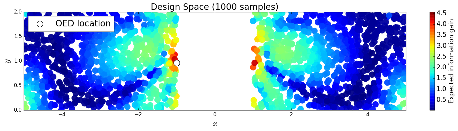 Figure 1
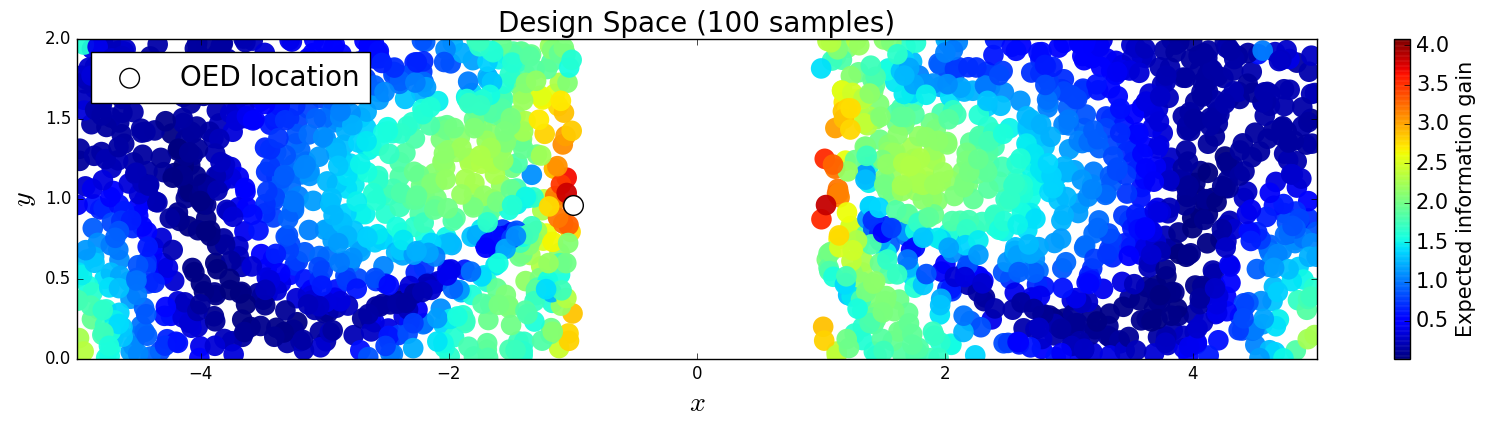 Figure 2
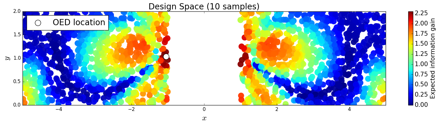 Figure 3
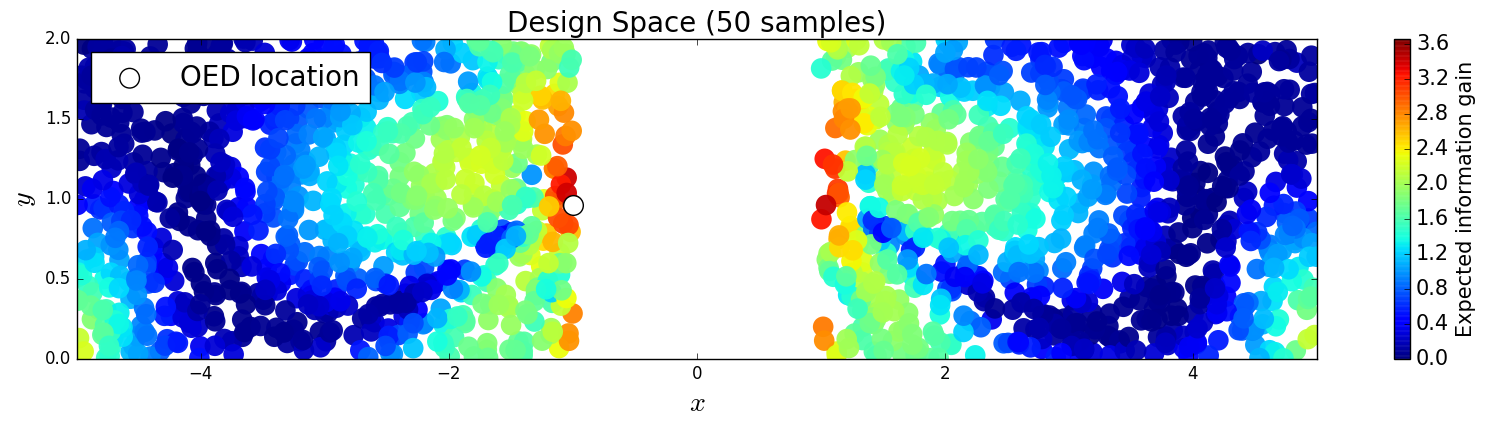 Figure 4
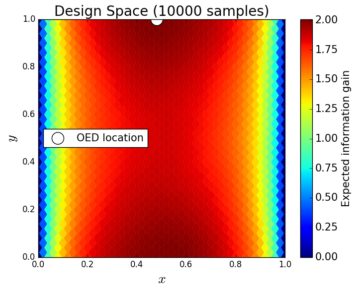 Figure 5
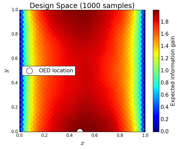 Figure 6
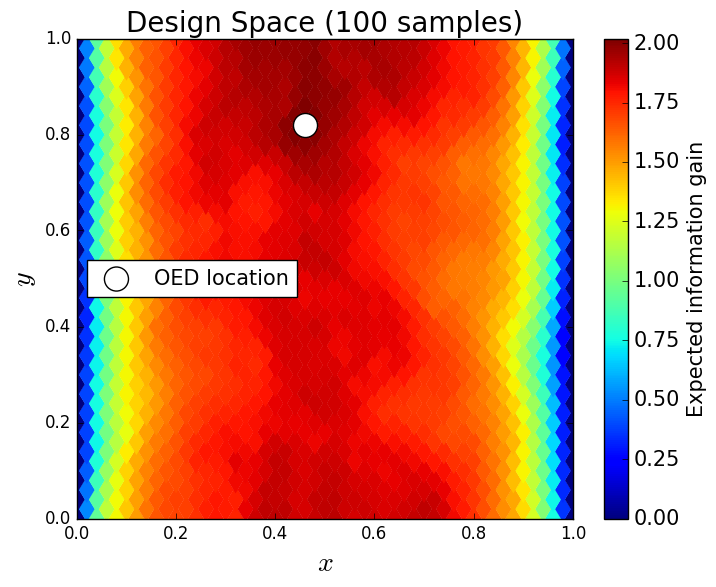 Figure 7
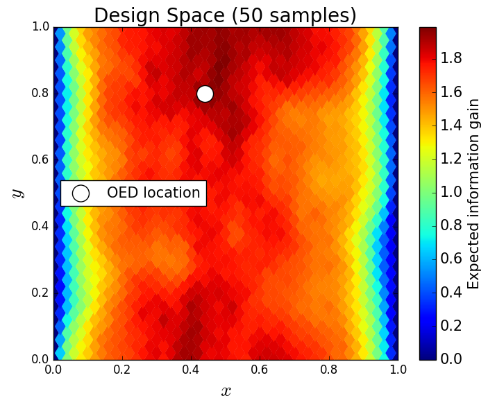 Figure 8
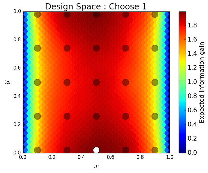 Figure 9
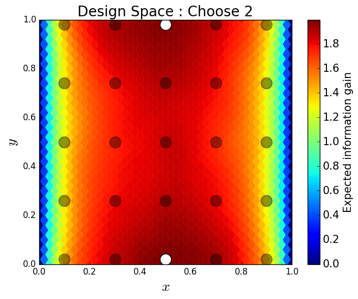 Figure 10
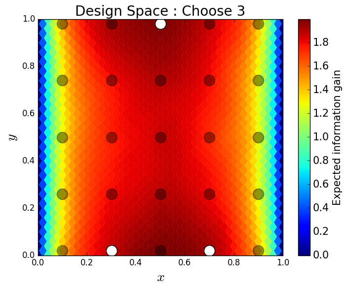 Figure 11
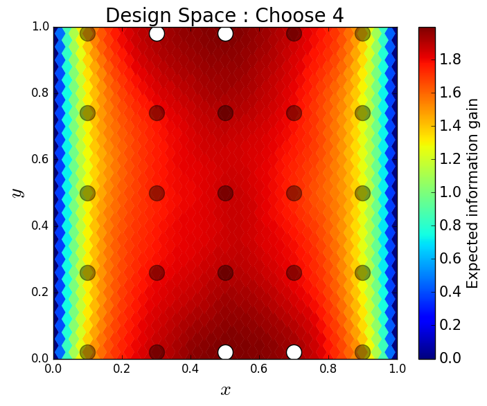 Figure 12
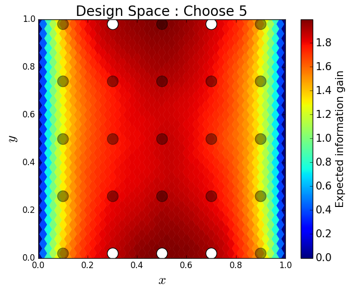 Figure 13
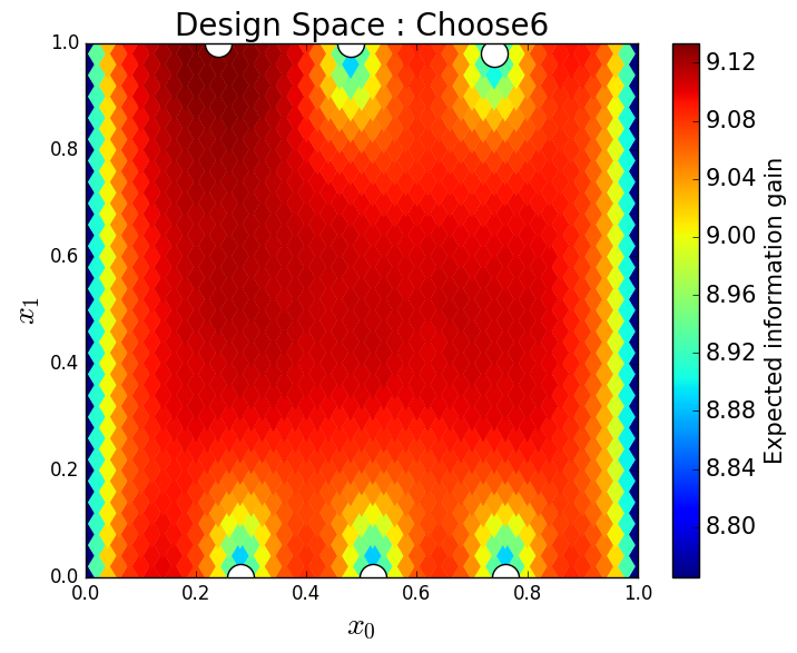 Figure 14
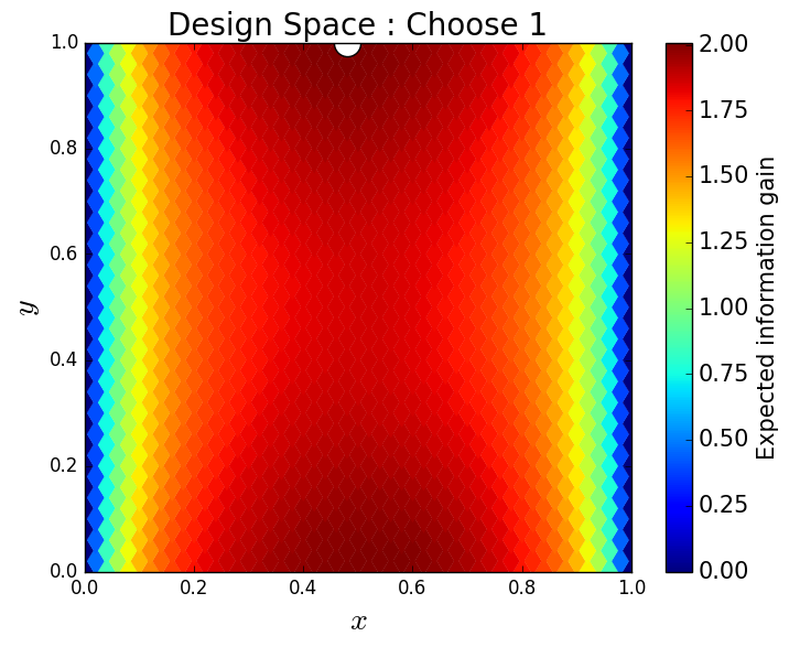 Figure 15
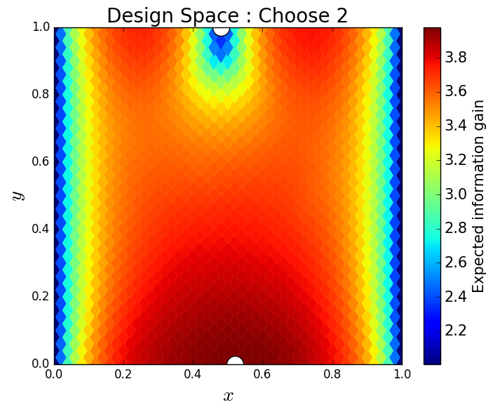 Figure 16
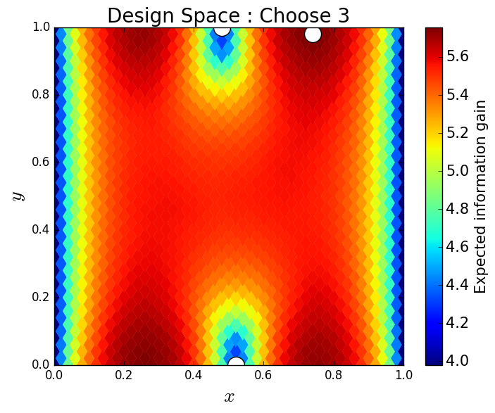 Figure 17
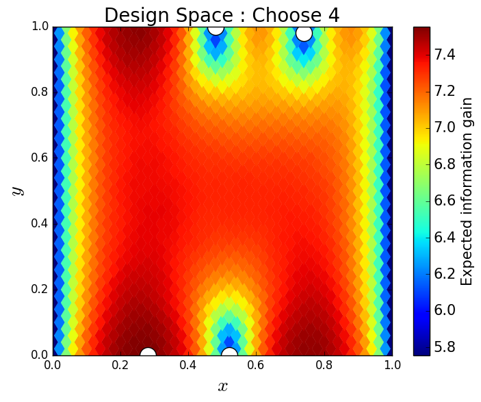 Figure 18
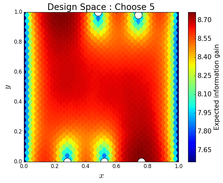 Figure 19
 Figure 20
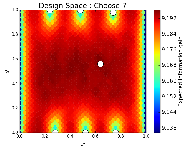 Figure 21
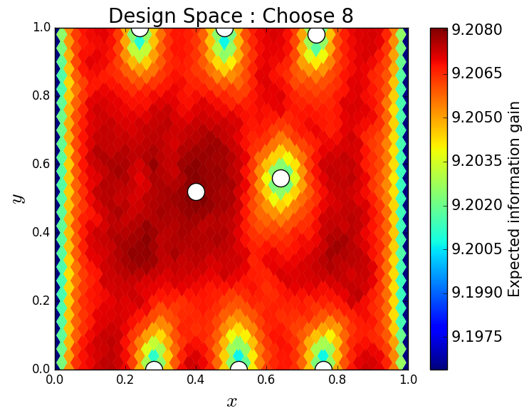 Figure 22
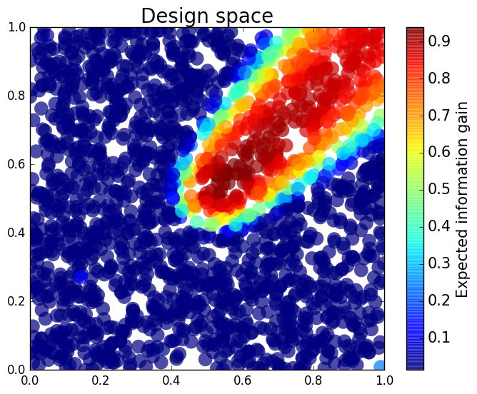 Figure 23
 Figure 24
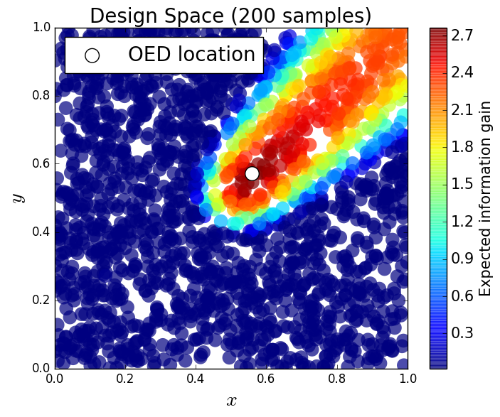 Figure 25
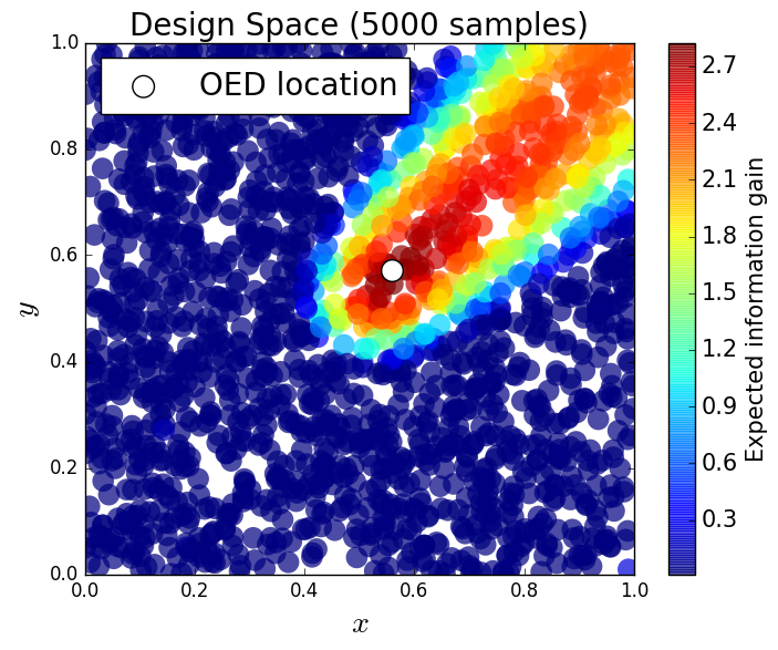 Figure 26
 Figure 27
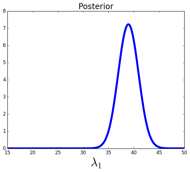 Figure 28
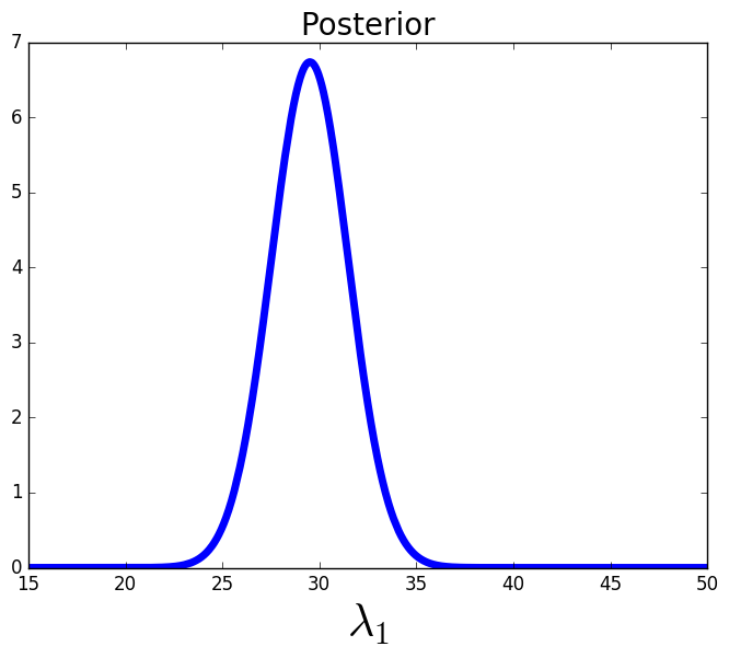 Figure 29
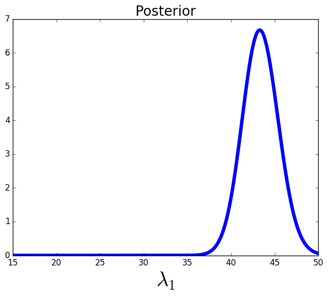 Figure 30
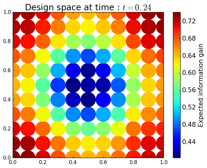 Figure 31
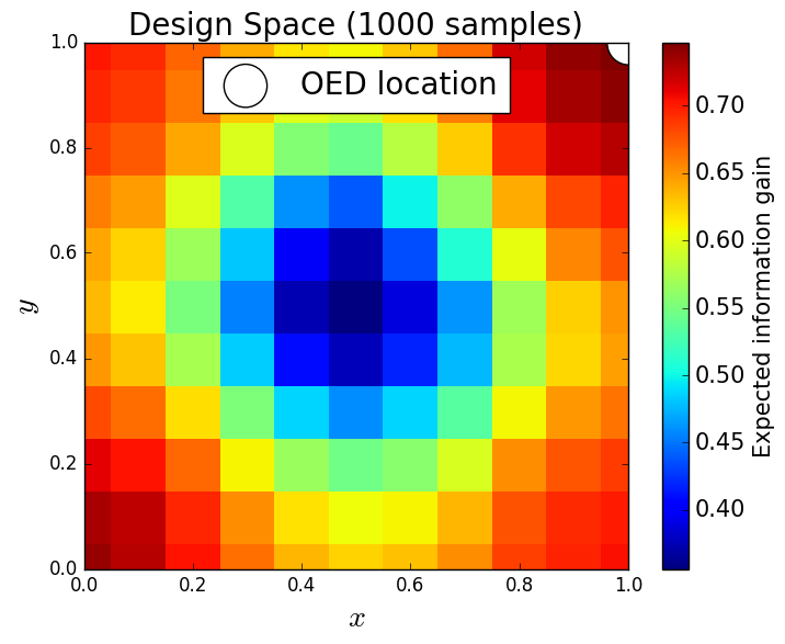 Figure 32
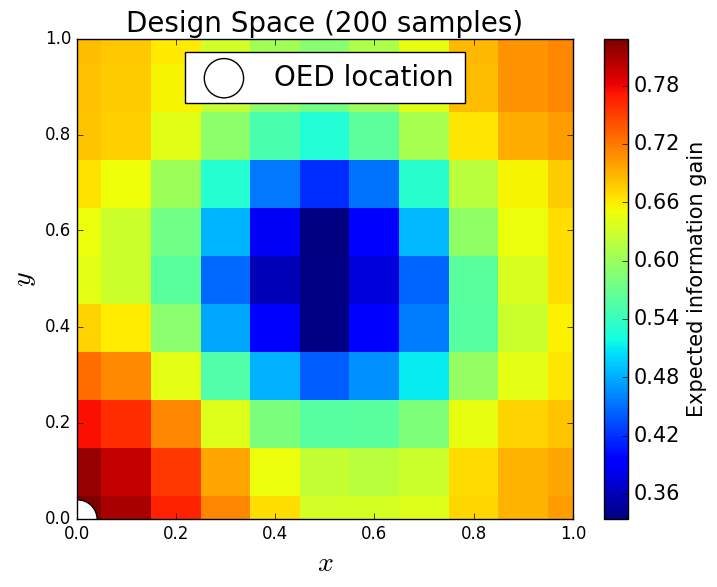 Figure 33
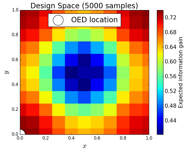 Figure 34
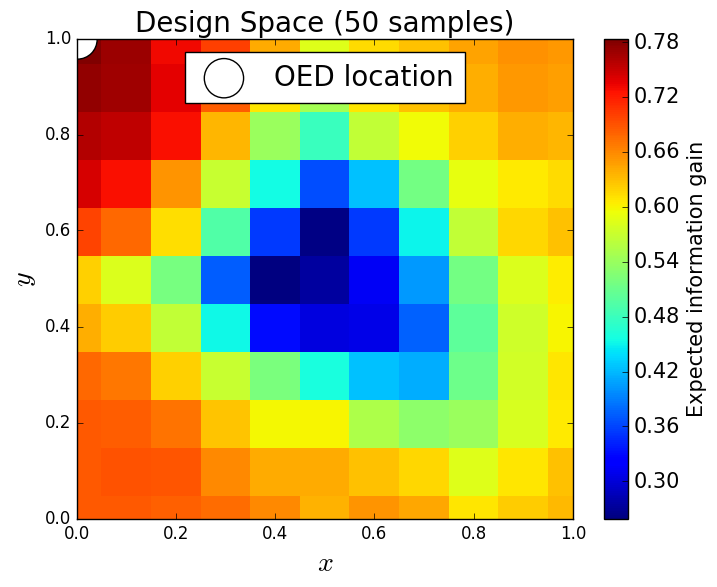 Figure 35
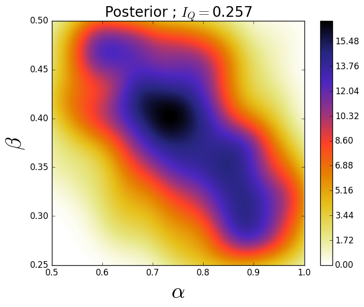 Figure 36
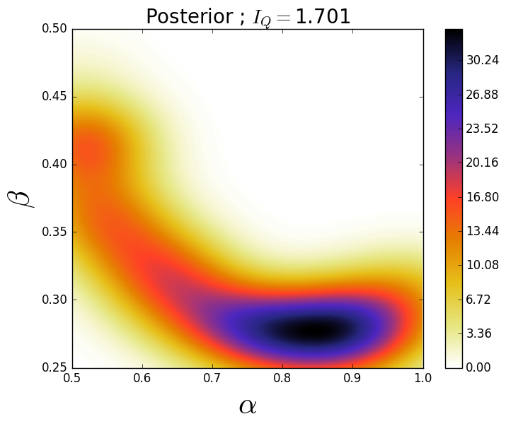 Figure 37
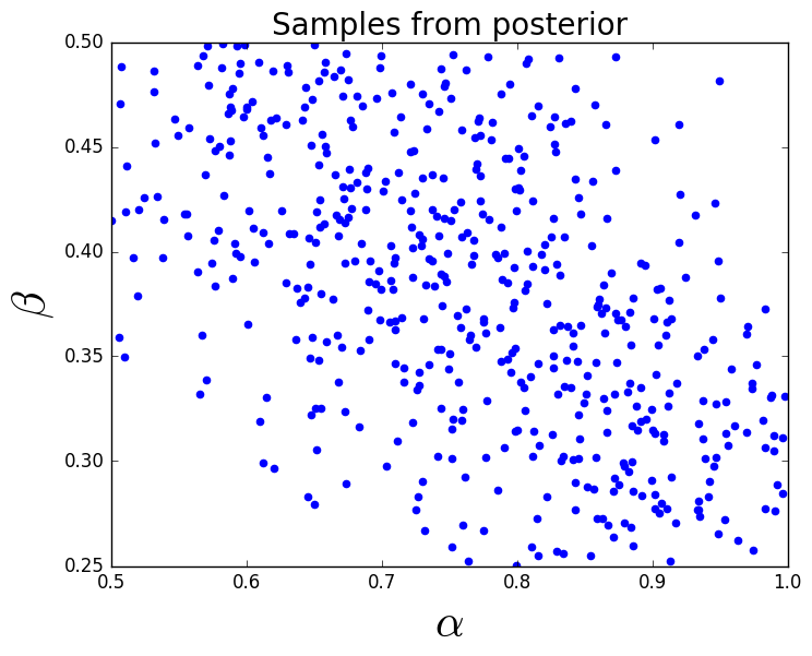 Figure 38
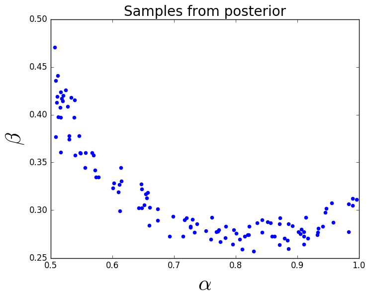 Figure 39
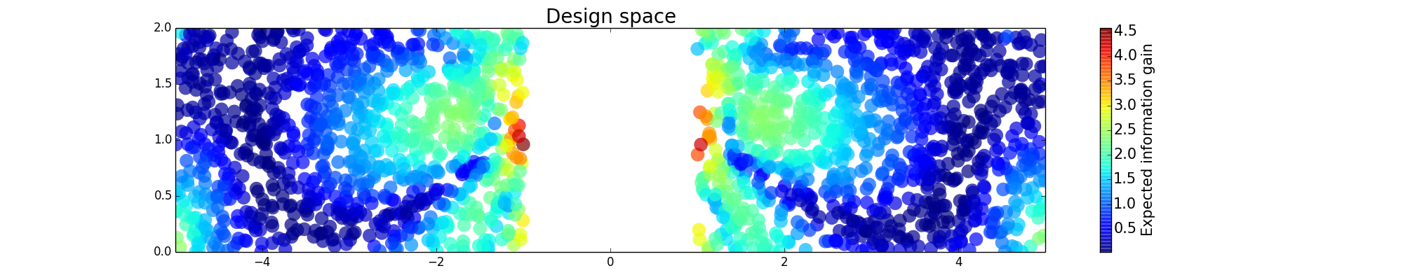 Figure 40
| Design Location | 50 | 200 | 1,000 | 5,000 |
|---|---|---|---|---|
| 2.758 | 2.767 | 2.815 | 2.826 | |
| 2.752 | 2.762 | 2.809 | 2.820 | |
| 2.729 | 2.736 | 2.782 | 2.793 | |
| 2.728 | 2.735 | 2.781 | 2.792 | |
| 2.726 | 2.733 | 2.779 | 2.790 |
| Design Location | 50 | 200 | 1,000 | 5,000 |
|---|---|---|---|---|
| 0.687 | 0.828 | 0.738 | 0.741 | |
| 0.653 | 0.713 | 0.747 | 0.740 | |
| 0.687 | 0.817 | 0.733 | 0.736 | |
| 0.687 | 0.810 | 0.728 | 0.735 | |
| 0.648 | 0.713 | 0.742 | 0.735 |
| Design Location | 10 | 50 | 100 | 1,000 |
|---|---|---|---|---|
| 2.303 | 3.662 | 4.085 | 4.569 | |
| 2.303 | 3.391 | 3.811 | 4.261 | |
| 2.303 | 3.437 | 3.839 | 4.256 | |
| 2.302 | 3.418 | 3.661 | 4.096 | |
| 2.277 | 3.246 | 3.544 | 3.813 |
| Design Location | 50 | 100 | 1,000 | 10,000 |
|---|---|---|---|---|
| 1.966 | 2.001 | 1.992 | 2.008 | |
| 1.952 | 1.963 | 1.993 | 2.007 | |
| 1.930 | 1.985 | 1.986 | 2.006 | |
| 1.777 | 1.915 | 1.999 | 2.006 | |
| 1.751 | 1.863 | 1.996 | 2.006 |
Peer Reviews
No public reviews on file for this paper yet. If you reviewed it on a platform where reviews are public (OpenReview, ICLR, NeurIPS, ICML), you can paste yours below so the community can read it here.
Videos
No videos yet. Explain this paper in a talk, walkthrough, or lecture? Add one.
\corauthor
J.D. Jakeman \[email protected]
\fundingSandia National Laboratories is a multimission laboratory managed and operated by National Technology and Engineering Solutions of Sandia, LLC., a wholly owned subsidiary of Honeywell International, Inc., for the U.S. Department of Energy’s National Nuclear Security Administration under contract DE-NA-0003525
Optimal Experimental Design Using A Consistent Bayesian Approach
S. Walsh Department of Mathematical and Statistical Sciences, University of Colorado Denver, Denver, CO 80202
T. Wildey Optimization and Uncertainty Quantification Department, Sandia National Labs, Albuquerque, NM
J. Jakeman\samethanks[2]
Abstract
We consider the utilization of a computational model to guide the optimal acquisition of experimental data to inform the stochastic description of model input parameters. Our formulation is based on the recently developed consistent Bayesian approach for solving stochastic inverse problems which seeks a posterior probability density that is consistent with the model and the data in the sense that the push-forward of the posterior (through the computational model) matches the observed density on the observations almost everywhere. Given a set a potential observations, our optimal experimental design (OED) seeks the observation, or set of observations, that maximizes the expected information gain from the prior probability density on the model parameters. We discuss the characterization of the space of observed densities and a computationally efficient approach for rescaling observed densities to satisfy the fundamental assumptions of the consistent Bayesian approach. Numerical results are presented to compare our approach with existing OED methodologies using the classical/statistical Bayesian approach and to demonstrate our OED on a set of representative PDE-based models.
1 Introduction
Experimental data is often used to infer valuable information about parameters for models of physical systems. However, the collection of experimental data can be costly and time consuming. For example, exploratory drilling can reveal valuable information about subsurface hydrocarbon reservoirs, but each well can cost upwards of tens of millions of US dollars. In such situations we can only afford to gather some limited number of experimental data, however not all experiments provide the same amount of information about the processes they are helping inform. Consequently, it is important to design experiments in an optimal way, i.e., to choose some limited number of experimental data to maximize the value of each experiment.
The first experimental design methods employed mainly heuristics, based on concepts such as space-filling and blocking, to select field experiments [14, 15, 32, 33, 38]. While these methods can perform well in some situations, these methods can be improved upon by incorporating any knowledge of the underlying physical processes being inferred or measured. Using physical models to guide experiment selection has been shown to drastically improve the cost effectiveness of experimental designs for a variety of models based on ordinary differential equations [26, 12, 6], partial differential equations [21] and differential algebraic equations [4]. When model observables are linear with respect to the model parameters the alphabetic optimality criteria are often used [19, 1, 17]. For example -optimality to minimize the average variance of parameter estimates, -optimality to maximize the differential Shannon entropy, or -optimality to minimize the maximum variance of model predictions. These criteria have been developed in both Bayesian and non-Bayesian settings [2, 1, 19, 3, 11, 28].
In this paper we focus attention on Bayesian methods for OED that can be applied to both linear and nonlinear models [30, 31, 35]. Specifically we pursue OEDs which are optimal for inferring model parameters on finite-dimensional spaces from experimental data observed at a set of sensor locations. In the context of OED for inference, analogues of the alphabetic criterion, for linear models have also been applied to nonlinear models [2, 29, 18, 21]. In certain situations, for example infinite-dimensional problems (random variables are random fields) or problems with computational expensive models, OED based upon linearizations of the model response and Laplace (Gaussian) approximations of the posterior distribution have been necessary [2, 29]. In other settings non-Gaussian approximations of the posterior have also been pursued [30, 31, 35, 28].
This manuscript presents a new approach for OED based upon consistent Bayesian inference, introduced in [8]. We adopt an approach for OED similar to the approach in [22] and seek an OED that maximizes the expected information gain from the prior to the posterior over the set of possible observational densities. Although our OED framework is Bayesian in nature, this approach is fundamentally different from the statistical Bayesian methods mentioned above. The aforementioned Bayesian OED methods use what we will refer to as the classical/statistical Bayesian approach for stochastic inference (see e.g., [36]) to characterize posterior densities that reflects an assumed error model. In contrast, consistent Bayesian inference assumes a probability density on the observations is given and produces a posterior density that is consistent with the model and the data in the sense that the push-forward of the posterior (through the computational model) matches the observed density almost everywhere. We direct the interested reader to [8] for a discussion on the differences between the consistent and statistical Bayesian approaches. Consistent Bayesian inference has some connections with measure-theoretic inference [7], which was used for OED in [9], but the two approaches make different assumptions and therefore typically give different solutions to the stochastic inverse problem.
The consistent Bayesian approach is appealing for OED since it can be used in an offline-online mode. Consistent Bayesian inference requires an estimate of the push-forward of the prior, which although expensive can be computed offline or obtained from archival simulation data. Once the push-forward of the prior is constructed, the posterior density can be approximated cheaply. Moreover, this push-forward of the prior does not depend on the density on the observations which enables a computationally efficient approach for solving multiple stochastic inverse problems for different densities on the observations. This can significantly reduce the cost of computing the expected information gain if the set of candidate observation is known a priori.
The main objectives in this paper are to derive an OED formulation using the consistent Bayesian framework and to present a computational strategy to estimate the expected information gained for an experimental design. The pursuit of a computationally efficient approach for coupling our OED method with continuous optimization techniques is an intriguing topic that we leave for future work. Here, we consider batch design over a discrete set of possible experiments. Batch design, also known as open-loop design, involves selecting a set of experiments concurrently such that the outcome of any experiment does not effect the selection of the other experiments. Such an approach is often necessary when one cannot wait for the results of one experiment before starting another, but is limited in terms of the number of observations we can consider.
The remainder of this paper is outlined as follows. In Section 2 we summarize the consistent Bayesian method for solving stochastic inverse problems. In Section 3 we discuss the information content of an experiment, and present our OED formulation based upon expected information gain. During the process of defining the expected information gain of a given experimental design, care must be taken to ensure that the model can predict all of our potential observed data. In Section 4 we discuss situations for which this assumption is violated and means for avoiding these situations. Numerical examples are presented in Section 5 and concluding remarks are provided in Section 6.
2 A Consistent Bayes formulation for stochastic inverse
problems
We are interested in experimental designs which are optimal for inferring model parameters from experimental data. Inferring model parameters for a single design and realization of experimental data is a fundamental component of producing such optimal designs. In this section we summarize the consistent Bayes method for parametric inference, originally presented in [8]. Although Bayesian in nature, the consistent Bayesian approach differs significantly from its classical Bayesian counterpart [36, 34, 25] which was used for OED in [22, 24, 10, 1, 2, 29, 28, 23]. We refer the interested reader to [8] for a full discussion of these differences.
2.1 Notation, Assumptions, and a Stochastic Inverse Problem
Let denote a deterministic model with solution that is an implicit function of model parameters . The set represents the largest physically meaningful domain of parameter values, and, for simplicity, we assume that is compact. In practice, modelers are often only concerned with computing a relatively small set of quantities of interest (QoI), , where each is a real-valued functional dependent on the model solution . Since is a function of parameters , so are the QoI and we write to make this dependence explicit. Given a set of QoI, we define the QoI map where denotes the range of the QoI map.
Assume and are measure spaces. We assume and are the Borel -algebras inherited from the metric topologies on and , respectively. The measures and are volume measures.
We assume that the QoI map is at least piecewise smooth implying that is a measurable map between the measurable spaces and . For any , we then have
[TABLE]
Furthermore, for any , although in most cases even when .
Finally, we assume that an observed probability measure, , is given on and is absolutely continuous with respect to , which implies it can be described in terms of an observed probability density, . The stochastic inverse problem is then defined as determining a probability measure, , described as a probability density, , such that, the push-forward measure agrees with . We use to denote the push-forward of through , i.e.,
[TABLE]
for all . Using this notation, a solution to the stochastic inverse problem is defined formally as follows:
Definition 1** (Consistency).**
Given a probability measure on that is absolutely continuous with respect and admits a density , the stochastic inverse problem seeks a probability measure on that is absolutely continuous with respect to and admits a probability density , such that the subsequent push-forward measure induced by the map, , satisfies
[TABLE]
for any . We refer to any probability measure that satisfies (1) as a consistent solution to the stochastic inverse problem.
Clearly, a consistent solution may not be unique, i.e., there may be multiple probability measures that are consistent in the sense of Definition 1. This is analogous to a deterministic inverse problem where multiple sets of parameters may produce the observed data. A unique solution may be obtained by imposing additional constraints or structure on the stochastic inverse problem. In this paper, such structure is obtained by incorporating prior information to construct a unique Bayesian solution to the stochastic inverse problem.
2.2 A Bayesian solution to the stochastic inverse problem
Following the Bayesian philosophy [37], we introduce a prior probability measure on that is absolutely continuous with respect to and admits a probability density . The prior probability measure encapsulates the existing knowledge about the uncertain parameters.
Assuming that is at least measurable, then the prior probability measure on , , and the map, , induce a push-forward measure on , which is defined for all ,
[TABLE]
We utilize the following expression for the posterior,
[TABLE]
which we describe in terms of a probability density given by
[TABLE]
We note that if , i.e., if the prior solves the stochastic inverse problem, then the posterior density will be equal to the prior density.
It was recently shown in [8] that the posterior given by (3) defines a consistent probability measure using a contour -algebra. When interpreted as a particular iterated integral of (4), the posterior defines a probability measure on in the sense of Definition 1, i.e., the push-forward of the posterior matches the observed probability density. Approximating the posterior density using the consistent Bayesian approach only requires an approximation of the push-forward of the prior probability on the model parameters, which is fundamentally a forward propagation of uncertainty. While numerous approaches have been developed in recent years to improve the efficiency and accuracy of the forward propagation of uncertainty using computational models, in this paper we only consider the most basic of methods, namely Monte Carlo sampling, to sample from the prior. We evaluate the computational model for each of the samples from the prior and use a standard kernel density estimator [40] to approximate the push-forward of the prior.
Given the approximation of the push-forward of the prior, we can evaluate the posterior at any point if we compute . This provides several possibilities for interogating the posterior. In Section 3.2, we compute on a uniform grid of points to visualize the posterior after we compute the push-forward of the prior. This does require additional model evaluations, but visualizing the posterior is rarely required and only useful for illustrative purposes in 1 or 2 dimensions. More often, we are interested in obtaining samples from the posterior. This is also demonstrated in Section 3.2 where the samples from the prior are either accepted or rejected using a standard rejection sampling procedure. For a given , we compute the ratio , where is an estimate of the maximum of the ratio over , and compare this value with a sample, , drawn from a uniform distribution on (0,1). If the ratio is larger than , then we accept the sample. We apply the accept-reject algorithm to the samples from the prior and therefore the samples from the posterior are a subset of the samples used to compute the push-forward of the prior. Since we have already computed for each of these samples, the computational cost to select a subset of the samples for the posterior is minimal. However, in the context of OED we are primarily interested in computing the information gained from the prior to the posterior which only involves integrating with respect to the prior (see Section 3.1) and does not require additional model evaluations or rejection sampling.
In practice, we prefer to use data that is sensitive to the parameters since otherwise it is difficult to infer useful information about the uncertain parameters. Specifically, if and the Jacobian of is defined a.e. in and is full rank a.e., then the push-forward volume measure is absolutely continuous with respect to the Lebesgue measure [8].
For the rest of this work we maintain the following assumptions needed to produce a unique consistent solution to the stochastic inverse problem:
(A1) We have a mathematical model and a description of our prior knowledge about the model input parameters,
(A2) The data exhibits sensitivity to the parameters a.e. in , hence, we use the Lebesgue measure as the volume measure on the data space,
(A3) The observed density is absolutely continuous with respect to the push-forward of the prior.
The assumption concerning the absolute continuity of the observed density with respect to the prior is essential to define a solution to the stochastic inverse problem [8]. While this assumption may appear rather abstract, it simply assures that the prior and the model can predict, with non-zero probability, any event that we have observed. Since the observed density and the model are assumed to be fixed, this is only an assumption on the prior.
In the remainder of this work, we focus on quantifying the value of these posterior densities. We use the Kullback-Leibler divergence [27, 39], to measure the information gained about the parameters from the prior to the posterior. We compute the expected information gain of a given set of QoI (a given experimental design), and then determine the OED to deploy in the field.
3 The information content of an
experiment
We are interested in finding the OED for inferring model input parameters. Conceptually, a design is informative if the posterior distribution of the model parameters is significantly different from the prior. To quantify the information gain of a design we use the Kullback-Leibler (KL) divergence [39] as a measure of the difference between a prior and posterior distribution. While the KL divergence is by no means the only way to compare two probability densities, it does provide a reasonable measure of the information gained in the sense of Shannon information [13] and is commonly used in Bayesian OED [24]. In this section we discuss how to compute the KL divergence and define our OED formulation based upon expected information gain over a specific space of possible observed densities.
3.1 Information gain: Kullback-Leibler divergence
Suppose we are given a description of the uncertainty on the observed data in terms of a probability density . This produces a unique solution to the stochastic inverse problem that is absolutely continuous with respect to the Lebesgue measure [8] and admits a probability density, . The KL divergence of the posterior from the prior (information gain), denoted , is given by
[TABLE]
Note that because is fixed, is simply a function of the posterior
[TABLE]
and from Eq. (4) the posterior is a function of the observed density. Therefore, we write as a function of the observed density,
[TABLE]
The observation that is a function of only allows us to define the expected information gain in Section 3.3 based on a specific space of observed densities.
Given a high dimensional parameter space, it may be computationally infeasible to accurately approximate the integral in Eq. (5). For example, a multi-variate normal density with unit variance in 100-dimensions has a maximum value of . However, we may write this integral in terms of densities on the data space evaluated at as follows
[TABLE]
where the second equality comes from a simple substitution using Eq. 4. Given a set of samples from the prior, we only need to compute the push-forward of the prior in the data space to approximate . This observation provides an efficient method for approximating given a high dimensional parameter space and a low dimensional data space. In fact, we found it convenient to use (8) whenever the prior is not uniform. In the consistent Bayesian formulation, we evaluate the model at the samples generated from the prior to estimate the push-forward of the prior. It is a computational advantage to also use these samples to integrate with respect to the prior rather than integrating with respect to the volume measure which would require additional model evaluations.
3.2 A motivating nonlinear system
Consider the following 2-component nonlinear system of equations with two parameters introduced in [7]:
[TABLE]
The first QoI is the second component, i.e., . The parameter ranges are given by and which are chosen as in [7] to induce an interesting variation in the QoI. We assume the observed density on is a truncated normal distribution with mean 0.3 and standard deviation of 0.01, see Figure 1 (right).
We generate 40,000 samples from the uniform prior and use a kernel density estimator (KDE) to construct an approximation to the resulting push-forward density, see Figure 1 (right). Then we use Eq. (4) to construct an approximation to the posterior density using the same 40,000 samples, see Figure 1 (left), and a simple accept/reject algorithm to generate a set of samples from the posterior, see Figure 1 (middle). We propagate this set of samples from the posterior through the model and approximate the resulting push-forward of the posterior density using a KDE. In Figure 1 (right) we see the push-forward of the posterior agrees quite well with the observed density. Notice the support of the posterior lies in a relatively small region of the parameter space. The information gain from this posterior is .
Next, we consider a different QoI to use in the inverse problem, and compare the support of its posterior to the one we just observed. Specifically consider,
[TABLE]
We assume the observed density on is a truncated normal distribution with mean 1.015 and standard deviation of 0.01. We approximate the push-forward density and the posterior using the same 40,000 samples and again generate a set of samples from the posterior and propagate these samples through the model to approximate the push-forward of the posterior, see Figure 2.
Although both and have the same standard deviation in their observed densities, clearly the two QoI produce very different posterior densities. The posterior corresponding to data from has a much larger region of support within the parameter space compared to that of the posterior corresponding to . This is quantified with the information gain from this posterior . Given these two maps, and , and the specified observed data on each of these data spaces, the data is more informative of the parameters than the data .
Next, we consider using the data from both and , , with the same means and standard deviations as specified above. Again, we approximate the push-forward density and the posterior using the same 40,000 samples, see Figure 3. With the information from both and we see a substantial decrease in the support of the posterior density. Intuitively, the support of the posterior using both and is the support of the posterior using intersected with the support of the posterior using . This is quantified in the information gain of this posterior .
In the scenario in which we can afford to gather data on both and , we benefit greatly in terms of reducing the uncertainties on the model input parameters. However, suppose we could only afford to gather one of these QoI in the field. Based on the information gain from each posterior, is more informative about the parameters than . However, consider a scenario in which the observed data has different means in both and . Due to the nonlinearities of the maps, it is not necessarily true that is still more informative than . If we do not know the mean of the data for either or , then we want to determine which of these QoI we expect to produce the most informative posterior.
3.3 Expected information gain
Optimal experimental design must select a design before experimental data becomes available. In the absence of data we use the simulation model to quantify the expected information gain of a given experimental design. Let denote the space of densities over . We want to define the expected information gain as some kind of average over this density space in a meaningful way. However, this is far too general of a space to use to define the expected information gain. This space includes densities that are unlikely to be observed in reality. Therefore, we restrict to be a space more representative of densities that may be observed in reality.
With no experimental data available to specify an observed density on a single QoI, we assume the density is a truncated Gaussian with a standard deviation determined by some estimate of the measurement instrument error. With Gaussians of (possibly) varying standard deviations specified for each QoI, this defines the shape of the observed densities we consider. We let denote the space of all densities of this shape centered in ,
[TABLE]
where is a truncated Gaussian function with mean and standard deviation . More details of this definition of are addressed in Section 4. We can easily generalize our description of . For example, we could also consider the standard deviation of the observed data to be uncertain, in which case we would also average over some interval of possible values for . However, in this work we only vary the center of the Gaussian densities.
Remark 1**.**
We can restrict in other ways as well. For example, if we expect the uncertainty in each QoI to be described by a uniform density, then we define the restriction on accordingly. This choice of characterization of the observed density space is largely dependent on the application. The only limitation is that we require the measure specified on the observed density space to be defined in terms of the push-forward measure, , as described below. In Section 5.2 we describe one approach for defining a restricted observed density space where the observed density of each QoI has a Gaussian profile and the standard deviations are functions of the magnitudes of each QoI.
The restriction of possible to this specific space of densities allows us to represent each density uniquely with a single point . Based on our prior knowledge of the parameters and the sensitivities of the map , the model informs us that some data are more likely to be observed than other data, this is seen in the plot of in Figure 3 (upper left). This implies we do not want to average over with respect to or , but rather with respect to the push-forward of the prior on , . This respects the prior knowledge of the parameters and the sensitivity information provided by the model. We define the expected information gain, denoted , as just described,
[TABLE]
From Eq. (5), itself is defined in terms of an integral. The expanded form for is then an iterated integral,
[TABLE]
where we make explicit that is a function of the observed density and, by our restriction of the space of observed densities in Eq. (9), therefore a function of . We utilize Monte Carlo sampling to approximate the integral in Eq. (10) as described in Algorithm 1.
Algorithm 1 appears to be a computationally expensive procedure since it requires solving stochastic inverse problems and, as noted in [8], approximating can be expensive. In [8] and in this paper we use kernel density estimation techniques to approximate which does not scale well as the dimension of increases [40]. On the other hand, for a given experimental design, we only need to compute this approximation once, as each in Step 4 of Algorithm 1 is computed using the same prior and map and, therefore, the same . In other words, the fact that the consistent Bayes method only requires approximating the push-forward of the prior implies that this information can be used to approximate posteriors for different observed densities without requiring additional model evaluations. This significantly improves the computational efficiency of the consistent Bayesian approach in the context of OED. We leverage this computational advantage throughout this paper by considering a discrete set of designs which allows us to compute the push-forward for all of the candidate designs simultaneously. Utilizing a continuous design space might require computing the push-forward for each iteration of the optimization algorithm, since the designs (locations of the observations) are not known a priori. The additional model simulations required to compute the push-forward of the prior at new design points might be intractable if the number of iterations is large, however the need for new simulations may be avoided, if the new observations can be extracted from archived state-space data. For example, if one stores the finite element solutions of a PDE at all samples of the prior at the first iteration of the design optimization, one can evaluate obsevations at new design locations, which are functionals of this PDE solution, via interpolation using the finite element basis.
3.4 Defining the OED
We are now in a position for define our OED formulation. Recall that our experimental design is defined as the set of QoI computed from the model and we seek the optimal set of QoI to deploy in the field. Given a physics based model, prior information on the model parameters, a space of potential experimental designs, and a generic description of the uncertainties for each QoI, we define our OED as follows.
Definition 2** (OED).**
Let represent the design space, i.e., the space of all possible experimental designs, and be a specific design. Then the OED is the that maximizes the expected information gain,
[TABLE]
As previously mentioned, the focus in this paper is on the utilization of the consistent Bayesian methodology within the OED framework, so we do not explore different approaches for solving the optimization problem given by Definition 2 and simply find the optimal design over a discrete set of candidate designs.
Remark 2**.**
Consistent Bayesian inference is potentially well suited to finding OED in continuous design spaces. Typically OED based upon statistical Bayesian methods uses Markov Chain Monte Carlo (MCMC) methods to characterize the posterior distribution. MCMC methods do not provide a functional form for the posterior but rather only provide samples from the posterior. Consequently, gradient-free or stochastic gradient-based optimization methods must be used to find the optimal design. In contrast consistent Bayesian inference provides a functional form for the posterior which allows the use of more efficient gradient based optimizers. Exploring the use of more efficient continuous optimization procedures will be the subject of future work.
4 Infeasible data
The OED procedure proposed in this manuscript is based upon consistent Bayesian inference which requires that the observed measure is absolutely continuous with respect to the push-forward measure induced by the prior and the model (assumption A3). In other words, any event that we observe with non-zero probability will be predicted using the model and prior with non-zero probability. During the process of computing , it is possible that we violate this assumption. Specifically, depending on the mean and variance of the observational density we may encounter such that , i.e., support of extends beyond the range of the map , see Figure 5 (upper right). In this section we discuss the causes of infeasible data and options for avoiding infeasible data when estimating an optimal experimental design.
4.1 Infeasible data and consistent Bayesian inference
When inferring model parameters using consistent Bayesian inference the most common cause for infeasible data is that the model being used to estimate the OED is inadequate. That is, the deviation between the computational model and reality is large enough to prohibit the model from predicting all of the observational data. The deviation between the model prediction and the observational data is often referred to as model structure error and can often be a major source of uncertainty. This is an issue of most if not all inverse parameter estimation problems [25]. Recently there has been a number of attempts to quantify this error (see e.g., [34]) however such approaches are beyond the scope of this paper. In the following we will assume that the model structure error does not prevent the model from predicting all the observational data.
4.2 Infeasible data and OED
To estimate an approximate OED we must quantify the expected information gain of a given experimental design (see Section 3.3). The expectation is over all possible normal observation densities with mean and variance , defined by the space (9). When the support of is bounded these densities may produce infeasible data. The effect of this violation increases as approaches the boundary of .
To remedy this violation of (A3) we must modify the set of observational densities. In this paper we choose to normalize over . We redefine the observed density space so that (A3) holds for each density in the space,
[TABLE]
where is a truncated Gaussian function with mean and standard deviation , and is the integral of over with respect to the Lebesgue measure on ,
[TABLE]
A similar approach for normalizing Gaussian densities over compact domains was taken in [5].
4.3 A nonlinear model with infeasible data
In this section, we use the nonlinear model introduced in Section 3.2 to demonstrate that infeasible data can arise from relatively benign assumptions. Suppose the observed density on is a truncated normal distribution with mean 0.3 and standard deviation of 0.04. In this one dimensional data space, this observed density is absolutely continuous with respect to the push-forward of the prior on , see Figure 4 (left). Next, suppose the observed density on is a truncated normal distribution with mean 0.982 and standard deviation of 0.01. Again, in this new one dimensional data space, this observed density is absolutely continuous with respect to the push-forward of the prior on , see Figure 4 (right). Both of these observe densities are dominated by their corresponding push-forward densities, i.e., the model can reach all of the observed data in each case.
However, consider the data space defined by both and and the corresponding push-forward and observed densities on this space, see Figure 5. The non-rectangular shape of the combined data space is induced by the nonlinearity in the model and the correlations between and . As we see in Figure 5, the observed density using the product of the 1-dimensional Gaussian densities is not absolutely continuous with respect to the push-forward density on , i.e., the support of extends beyond the support of . Referring to Eq. (13), we normalize this observed density over , see Figure 5 (right). Now that the new observed density obeys the assumptions needed, we could solve the stochastic inverse problem as described in Section 2.
4.4 Computational considerations
The main computational challenge in the consistent Bayesian approach is the approximation of the push-forward of the prior. Following [8], we use Monte Carlo sampling for the forward propagation of uncertainty. While the rate of convergence is independent of the number of parameters (dimension of ), the accuracy in the statistics for the QoI may be relatively poor unless a large number of samples can be taken. Alternative approaches based on surrogate models can significantly improve the accuracy, but are generally limited to small number of parameters. We also employ kernel density estimation techniques to construct a non-parametric approximation of the push-forward density, but it is well-known that these techniques do not scale well with the number of observations (dimension of ) [40].
Next, we address the computational issue of normalizing , i.e., , over . From the plot of in Figure 5 (left) it is clear the data space may be a complex region. Normalizing , as in Figure 5 (right), over would be computationally expensive. Fortunately, the consistent Bayesian approach provides a means to avoid this expense. Note that from Eq. (3) we have,
[TABLE]
where which implies,
[TABLE]
Therefore, normalizing over is equivalent to solving the inverse problem and then normalizing (where we use the tilde over to indicate this function does not integrate to 1 because we have violated (A3)) over . Although may not always be a generalized rectangle, (A1) implies we have a clear definition of and therefore can efficiently integrate over and then normalize by
[TABLE]
In fact, this normalization factor can be estimated without additional model evaluations and without using the values of the prior or the posterior, which may not be usable in high-dimensional spaces. We observe that
[TABLE]
Thus, we can use the values of and computed for the samples generated from the prior, which were used to estimate the push-forward of prior, to integrate with respect to the prior.
5 Numerical examples
In this section we consider several models of physical systems. First, we consider a stationary convection-diffusion model with a single uncertain parameter controlling the magnitude of the source term. Next, we consider a transient transport model with a two dimensional parameter space determining the location of the source of a contaminant. Then, we consider a inclusion problem in computational mechanics where two uncertain parameters control the shape of the inclusion. Finally, we consider a high-dimensional example of single-phase incompressible flow in porous media where the uncertain permeability field is given by a Karhunen-Loeve expansion [42].
In each example, we have a parameter space , a set of possible QoI, and a specified number of QoI we can afford to gather during the experiment. This in turn defines a design space and we let represent a single experimental design and the corresponding data space. For each experimental design, we let represent the standard deviations defined by the uncertainties in each QoI that compose and represent the observed density space.
All of these examples have continuous design spaces, so we approximate the OED by selecting the OED from a large set of candidate designs. This approach was chosen because it is much more efficient to perform the forward propagation of uncertainty using random sampling only once and to compute all of the candidate measurements for each of these random samples. Alternatively, one could pursue a continuous optimization formulation which would require a full forward propagation of uncertainty for each new design. As mentioned in Section 3.4, one could limit the number of designs using a gradient-based or Newton-based optimization approach, but this is beyond the scope of this paper.
5.1 Stationary convection-diffusion: uncertain source amplitude
In this section we consider a convection-diffusion problem with a single uncertain parameter controlling the magnitude of a source term. This example serves to demonstrate that the OED formulation gives intuitive results for simple problems.
5.1.1 Problem setup
Consider a stationary convection diffusion model on a square domain:
[TABLE]
with
[TABLE]
where , is the concentration field, the diffusion coefficient , the convection vector , and is a Gaussian source with the following parameters: is the location, is the amplitude, is the width. We impose homogeneous Neumann boundary conditions on (right and top boundaries) and homogeneous Dirichlet conditions on (left and bottom boundaries). For this problem, we choose , and . We let be uncertain within , thus the parameter space for this problem is . Hence, our goal is to gather some limited amount of data that provides the best information about the amplitude of the source, i.e., reduces our uncertainty in . To approximate solutions to the PDE in Eq. 18 given a source amplitude , we use a finite element discretization with continuous piecewise bilinear basis functions defined on a uniform () spatial grid.
5.1.2 Results
We assume that we have limited resources for gathering experimental data, specifically, we can only afford to place one sensor in the domain to gather a single concentration measurement. Our goal is to place this single sensor in to maximize the expected information gained about the amplitude of the source. We discretize using 2,000 uniform random points which produces a design space with 2,000 possible experimental designs. For this problem, we let the uncertainty in each QoI be described by a truncated Gaussian profile with a fixed standard deviation of 0.1. This produces observed density spaces, , as described in Eq. 13.
We generate 5,000 uniform samples from the prior and simulate measurements of each QoI for each of these 5,000 samples. We consider approximate solutions to the OED problem using subsets of the 5,000 samples of size 50, 200, 1,000 and 5,000. For each experimental design, we calculate using Algorithm 1 and plot as a function of the discretized design space in Figure 6. Notice the expected information gain is greatest near the center of the domain (near the location of the source) and in the direction of the convection vector away from the source. This result matches intuition, as we expect data gathered in regions of the domain that exhibit sensitivity to the parameters to produce high expected information gains.
We note that, for this example, a sufficiently accurate approximation to the design space and the OED is obtained using only 50 samples corresponding to 50 model evaluations. In Table 1 we show the top 5 experimental designs (computed using the full set of 5,000 samples) and corresponding for each set of samples.
5.2 Time dependent diffusion: uncertain source location
In this section, we compare results from a statistical Bayesian formulation of OED to the formulation described in this paper. Specifically, we consider the model in [22] where the author uses a classical Bayesian framework for OED to determine the optimal placement of a single sensor that maximizes the expected information about the location of a contaminant source.
5.2.1 Problem setup
Consider a contaminant transport model on a square domain:
[TABLE]
with
[TABLE]
where , is the space-time concentration field, we impose homogeneous Neumann boundary conditions along with a zero initial condition, and is a Gaussian source with the following parameters: is the location, is the intensity, is the width, and is the shutoff time.
Our goal is to gather some limited amount of data that provides the best information about the location of the source, i.e., reduces our uncertainty in . For this problem, we choose and and let be uncertain within such that . To approximate solutions to the PDE in Eq. 19 given a location of , i.e., a given , we use a finite element discretization with continuous piecewise bilinear basis functions defined on a uniform () spatial grid and backward Euler time integration with a step size (100 time steps).
5.2.2 Results
We assume that we have limited resources for gathering experimental data, specifically, we can only afford to place one sensor in the domain and can only gather a single concentration measurement at time . Our goal is to place this single sensor in to maximize the expected information gained about the location of the contaminant source. For simplicity, we discretize using an regular grid of points which produces a design space with 121 possible experimental designs. We let the uncertainty in each QoI be described by a Gaussian profile with a standard deviation that is a function of the magnitude of the QoI, i.e.,
[TABLE]
where is the dimension of the data space. This produces observed density spaces, , that consist of truncated Gaussian functions with varying standard deviations,
[TABLE]
We generate 5,000 uniform samples from the prior and simulate measurements of each QoI for each of these 5,000 samples. We consider approximate solutions to the OED problem using subsets of the 5,000 samples of size 50, 200, 1,000 and 5,000. For each experimental design, we use this data to calculate using Algorithm 1 and plot as a function of the discretized design space in Figure 7. Notice the expected information gain is greatest near the corners of the domain and smallest near the center, this is consistent with [22]. In Table 2 we show the top 5 experimental designs, approximated using the full set of 5,000 samples, and corresponding for each set of samples.
In Figure 8 we consider three different posteriors computed using data from the OED approximated using 5,000 samples, i.e., data gathered by a sensor placed in the bottom left corner of the domain, where each posterior corresponds to a different possible location of the source. We see varying levels of information gain in these three scenarios, reiterating the point that we choose the OED based on the average of these information gains, .
Remark 3**.**
*Although many of the results in this section seem to match our intuition about which measurement locations should produce high expected information gains, this may not always be the case. In particular, we have found that our results can depend on our choice of the variance in the the observed densities . If is chosen to be large relative to the range of a data space, then the posteriors produced as we average over are all nearly the same and potentially produce unusually high information gains when the observed densities have substantial support over regions of the data space with very small probability (very small values of the push-forward of the prior). Another way to think of this is the push-forward densities have high entropy and because is large is very close to uniform and this produces posterior densities with high information gains. If is chosen to be small relative to the range of the data space, i.e., if we expect the experiments to be informative, we do not encounter this issue because we are integrating over with respect to the push-forward measure so most of our potential observed data lies in high probability regions of the data space. *
5.3 A Parameterized Inclusion
In this section, we consider a simple problem in computational mechanics where the precise boundary of an inclusion is uncertain. We parameterize the inclusion and seek to determine the location to place a sensor that will maximize the information gained regarding the shape of the inclusion. We use a linear elastic formulation to model the response of the media to surface forces and measure horizontal stress at each sensor location. We assume that the material properties (Poisson ratio and Young’s modulus) are different inside the inclusion and that these properties are known a prior.
5.3.1 Problem setup
Consider a linear elastic plane strain model,
[TABLE]
where is given by the linear elastic constitutive relation,
[TABLE]
We express this relation in terms of the Lamé parameters, and , which are related to the Poisson ratio, , and Young’s modulus, , via the following expressions,
[TABLE]
Now assume that there is an inclusion within the media defined by an ellipse
[TABLE]
where and is uniformly distributed on and is uniformly distributed on . The material properties are assumed to be known and are given by,
[TABLE]
These material properties were not chosen to emulate any particular materials, just to demonstrate the proposed OED formulation.
Next let us impose homogeneous Dirichlet boundary conditions on the bottom boundary and stress free boundary conditions on the sides, and impose a uniform traction in the y-direction along the top boundary (). And finally assume that we can probe the media and measure the horizontal stress at a given sensor location. We do not want to puncture the inclusion, so we only consider sensor locations outside the bounds on the inclusion. Equation 22 was solved using a finite element discretization with piecewise linear basis functions defined on a uniform mesh resulting in a system with 64,962 degrees of freedom. The computational model is implemented using the Trilinos toolkit [20] and each realization of the model requires approximately 1 second using 8 processors.
5.3.2 Results
As in previous examples, we assume that we have limited resources for gathering experimental data, specifically, we can only afford to place one sensor in the domain to gather a single stress measurement. Our goal is to place this single sensor to maximize the expected information gained about the shape of the inclusion. We select 2,000 random sensor locations (outside the inclusion bounds) which produces a design space with 2,000 possible experimental designs. For this problem, we let the probability density for the QoI be described by a truncated Gaussian profile with a fixed standard deviation of 0.001. We generate 1,000 uniform samples from the prior and compute the horizontal stress at each sensor location for each of these 1,000 samples.
First, we compare the posterior densities for two sensor locations, and , under the assumption that we have already gathered data at these sensor locations. The purpose here is to demonstrate that we obtain different posterior densities and therefore gain different information from each sensor. The first sensor is further from the inclusion so we expect that the data from the second sensor will constrain the posterior more than the data from the first. In Figures 10 and 11, we plot the samples from the posterior and the corresponding kernel density estimate of the posterior for the first and second sensor locations respectively. It is clear that measuring the horizontal stress closer to the inclusion increases the information gained from the prior to the posterior.
We consider approximate solutions to the OED problem using subsets of the 1,000 samples of size 10, 50, 100 and 1,000. For each experimental design, we use this data to calculate using Algorithm 1 and plot as a function of the discretized design space in Figure 12. Notice the expected information gain is greatest near the bottom of the domain near the inclusion and is reasonably symmetric around the inclusion. Also note that the expected information gain is relatively large in the bottom corners of the domain. This is due to the choice of boundary conditions for the model which induces a large amount of stress in these corners. In Table 2 we show the top 5 experimental designs, approximated using the full set of 1,000 samples, and corresponding for each set of samples.
5.4 A Higher-Dimensional Porous Media Example with Uncertain Permeability
In this section, we consider an example of single-phase incompressible flow in porous media with a Karhunen-Loéve expansion of the uncertain permeability field. The purpose of this example is to demonstrate the OED formulation on a problem with a high-dimensional parameter space and more than one sensor.
5.4.1 Problem setup
Consider a single-phase incompressible flow model:
[TABLE]
Here, is the pressure field and is the permeability field which we assume is a scalar field given by a Karhunen-Loéve expansion of the log transformation, , with
[TABLE]
where is the mean field. We assume the mean removed random media is given by a Gaussian process which implies that the are mutually uncorrelated random variables with zero mean and unit variance [16, 41]. The eigenvalues, , and eigenfunctions, , are computed numerically using the following covariance function,
[TABLE]
where and denote the variance and correlation length in the i spatial direction respectively. We assume a correlation length of in each spatial direction and truncate the expansion at 100 terms. This choice of truncation is purely for the sake of demonstration. In practice, the expansion is truncated once a sufficient fraction of the energy in the eigenvalues is retained [42, 16]. This truncation gives 100 uncorrelated random variables, , with zero mean and unit variance which implies . To approximate solutions to the PDE in Eq. 23 we use a finite element discretization with continuous piecewise bilinear basis functions defined on a uniform () spatial grid.
5.4.2 Results
In this section, we present approximate solutions to several different design problems. We begin with the familiar problem of choosing a single sensor location within the physical domain. Then, we consider approximating the optimal location of a second sensor given the location of the first sensor. In this way, we solve the greedy OED problem and determine the greedy optimal locations of 1-8 sensors within the physical domain. We then consider solving the ehaustive OED problem where we limit the sensors to 25 locations and consider determining the optimal location of 5 available sensors.
First, assume that we have limited resources for gathering experimental data, specifically, we can only afford to place one sensor in the domain to gather a single pressure measurement. Our goal is to place this single sensor in to maximize the expected information gained about the amplitude of the source. We discretize using 1,301 pionts on a grid which produces a design space with 1,301 possible experimental designs. For this problem, we let the uncertainty in each QoI be described by a truncated Gaussian profile with a fixed standard deviation of 0.01. This produces observed density spaces, , as described in Eq. 13.
We generate 10,000 samples from the prior and simulate measurements of each QoI. We consider approximate solutions to the OED problem using subsets of the 10,000 samples of size 50, 100, 1,000 and 10,000. For each experimental design, we calculate using Algorithm 1 and plot as a function of the discretized design space in Figure 13. Notice the expected information gain is greatest near the top and bottom of the domain away from the left and right edges. This result matches intuition, as we expect data gathered near the left and right edges to be less informative given the Dirichlet boundary condition imposed on those boundaries. We note that, for this example, a sufficiently accurate approximation to the design space and the OED is obtained using only 1,000 samples corresponding to 1,000 model evaluations. In Table 1 we show the top 5 experimental designs (computed using the full set of 10,000 samples) and corresponding for each set of samples.
Next, we consider the greedy OED problem of placing 8 sensors within the physical domain. We choose to use all of the available 10,000 samples to solve this problem. In Figure 14, we see the design space as a function of the previously determined locations of placed sensors. We observe a strong symmetry to this problem, as is expected due to the symmetry of the physical process defined on this domain with the given boundary conditions. In the bottom right of Figure 14, notice the very small range of the color bar indicating the possible values of the expected information gain. This suggests, for this example, we expect there is a limit on the number of useful sensor locations for informing likely parameter values.
Lastly, we consider the exhaustive OED problem of placing 5 sensors within the physical domain and, for computational feasibility, restrict the possible locations of these 5 sensors to 25 points in the physical domain, see Figure 15. We choose to use 1,000 samples to solve this problem. In Figure 15, we plot the design space for a single sensor location using these 1,000 samples and show the optimal location of 1, 2, 3, 4 and 5 sensors. The results are quite similar to the greedy results previously described.
6 Conclusion
In this manuscript, we developed an OED formulation based on the recently developed consistent Bayesian approach for solving stochastic inverse problems. We used the Kullback-Leibler divergence and the posterior obtained using consistent Bayesian inference to measure the information gain of a design and present a discrete optimization procedure for choosing the optimal experimental design that maximizes the expected information gain. The optimization procedure presented in this paper is limited in terms of the number of observations we can consider, but was chosen to focus attention on the definition and approximation of the expected information gained. More efficient strategies, utilizing gradient-based methods on continuous design spaces, will be pursued in a future work. We discussed a characterization of the space of observed densities needed to compute the expected information gain and a computationally efficient approach for rescaling observed densities to satisfy the requirements of the consistent Bayesian approach. Numerical examples were given to highlight the properties and utility of our approach.
7 Acknowledgments
J.D. Jakeman’s work was supported by DARPA EQUIPS. Sandia National Laboratories is a multimission laboratory managed and operated by National Technology and Engineering Solutions of Sandia, LLC., a wholly owned subsidiary of Honeywell International, Inc., for the U.S. Department of Energy’s National Nuclear Security Administration under contract DE-NA-0003525.
The reference list from the paper itself. Each links out to its DOI / PubMed record.
- 1[1] Alen Alexanderian, Noemi Petra, Georg Stadler, and Omar Ghattas. A-optimal design of experiments for infinite-dimensional bayesian linear inverse problems with regularized 𝓁 0 subscript 𝓁 0 {\cal l}_{0} -sparsification. SIAM Journal on Scientific Computing , 36(5):A 2122–A 2148, 2014.
- 2[2] Alen Alexanderian, Noemi Petra, Georg Stadler, and Omar Ghattas. A fast and scalable method for a-optimal design of experiments for infinite-dimensional bayesian nonlinear inverse problems. SIAM Journal on Scientific Computing , 38(1):A 243–A 272, 2016.
- 3[3] A.C. Atkinson and A.N. Donev. Optimum Experimental Designs . Oxford University Press, 1992.
- 4[4] Irene Bauer, Hans Georg Bock, Stefan Körkel, and Johannes P. Schlöder. Numerical methods for optimum experimental design in {DAE} systems. Journal of Computational and Applied Mathematics , 120(1–2):1 – 25, 2000.
- 5[5] Fabrizio Bisetti, Daesang Kim, Omar Knio, Quan Long, and Raul Tempone. Optimal bayesian experimental design for priors of compact support with application to shock-tube experiments for combustion kinetics. International Journal for Numerical Methods in Engineering , 108(2):136–155, 2016.
- 6[6] Hans Georg Bock, Stefan Körkel, and Johannes P. Schlöder. Parameter Estimation and Optimum Experimental Design for Differential Equation Models , pages 1–30. Springer Berlin Heidelberg, Berlin, Heidelberg, 2013.
- 7[7] J. Breidt, T. Butler, and D. Estep. A computational measure theoretic approach to inverse sensitivity problems I: Basic method and analysis. SIAM J. Numer. Analysis , 49:1836–1859, 2012.
- 8[8] T. Butler, J. Jakeman, and T. Wildey. A consistent bayesian formulation for stochastic inverse problems based on push-forward measures. ar Xiv:1704.00680 , 2016. Submitted to SIAM J. Sci. Comput.