Quantifying gerrymandering using the vote distribution
Gregory S. Warrington

TL;DR
This paper introduces a new, simple measure of partisan asymmetry for detecting gerrymandering that overcomes limitations of the efficiency gap and is applicable to various district plans.
Contribution
The authors propose a novel measure of partisan asymmetry that is easy to compute, related to packing and cracking, and avoids proportional representation issues.
Findings
The new measure effectively identifies gerrymandered districts.
Application to US plans reveals potential gerrymandering cases.
The generalized efficiency gap offers an alternative assessment method.
Abstract
To assess the presence of gerrymandering, one can consider the shapes of districts or the distribution of votes. The "efficiency gap," which does the latter, plays a central role in a 2016 federal court case on the constitutionality of Wisconsin's state legislative district plan. Unfortunately, however, the efficiency gap reduces to proportional representation, an expectation that is not a constitutional right. We present a new measure of partisan asymmetry that does not rely on the shapes of districts, is simple to compute, is provably related to the "packing and cracking" integral to gerrymandering, and that avoids the constitutionality issue presented by the efficiency gap. In addition, we introduce a generalization of the efficiency gap that also avoids the equivalency to proportional representation. We apply the first function to US congressional and state legislative plans from…
Click any figure to enlarge with its caption.
 Figure 1
 Figure 2
 Figure 3
 Figure 0
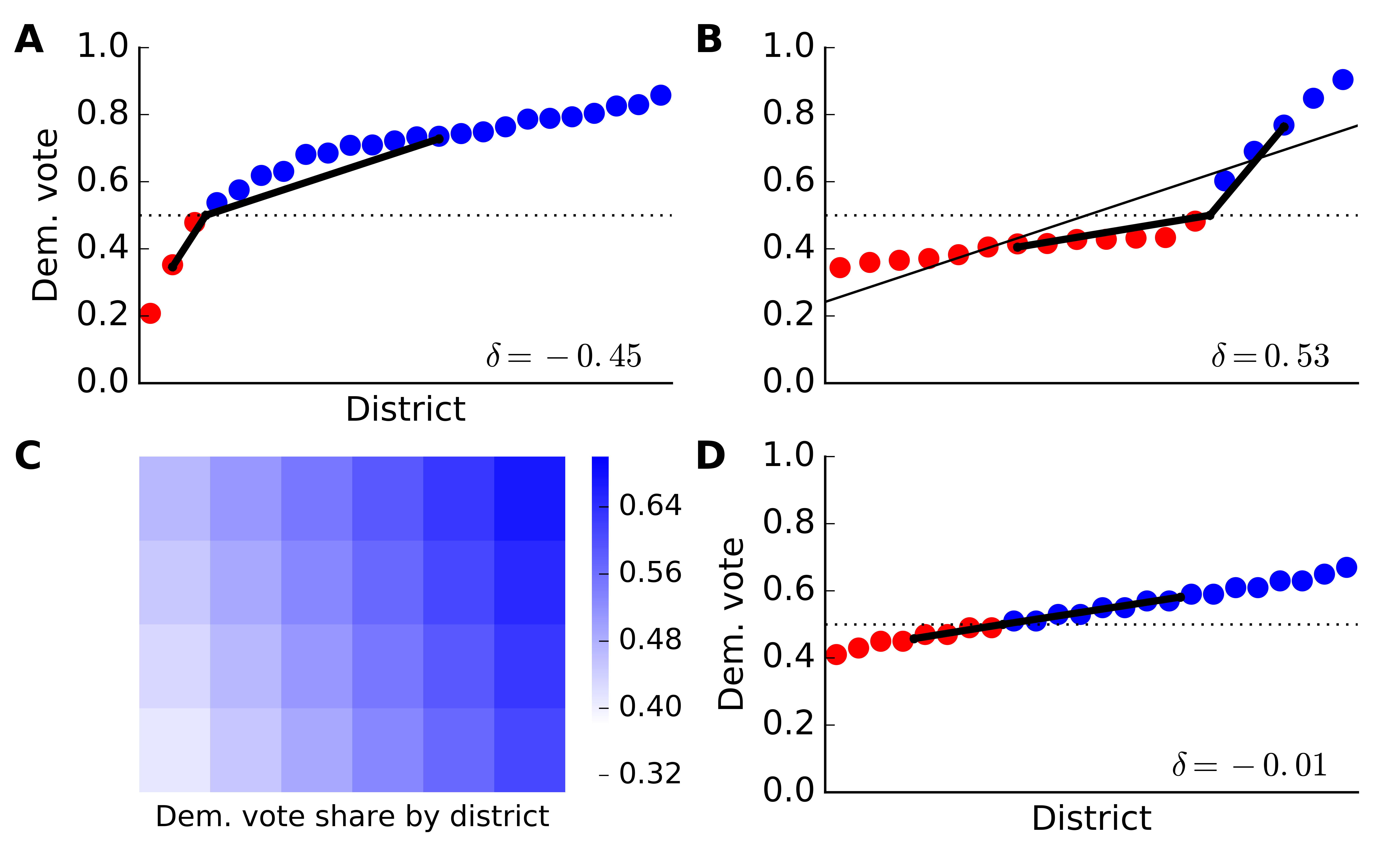 Figure 1
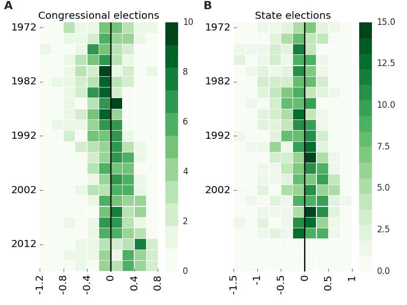 Figure 2
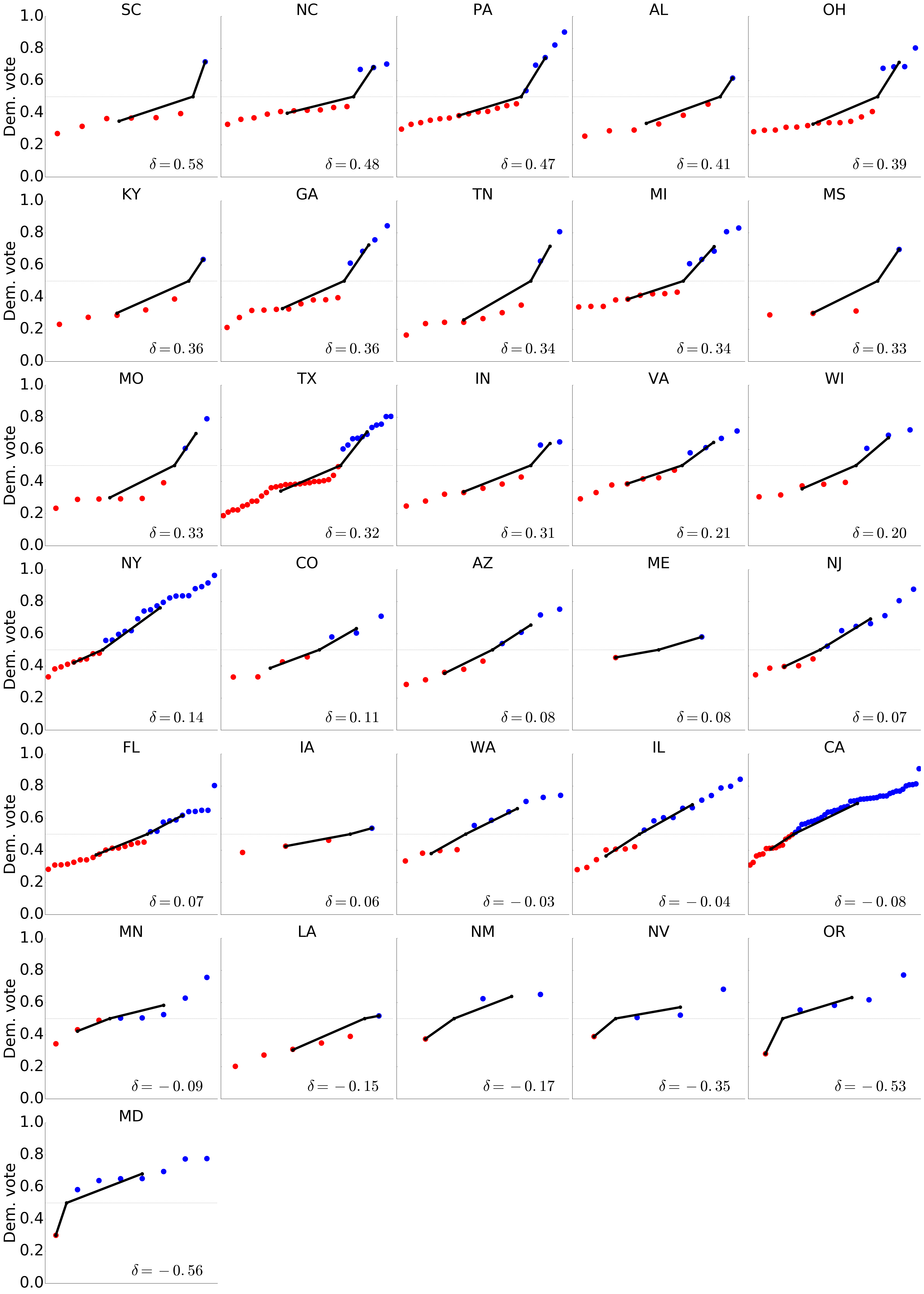 Figure 7
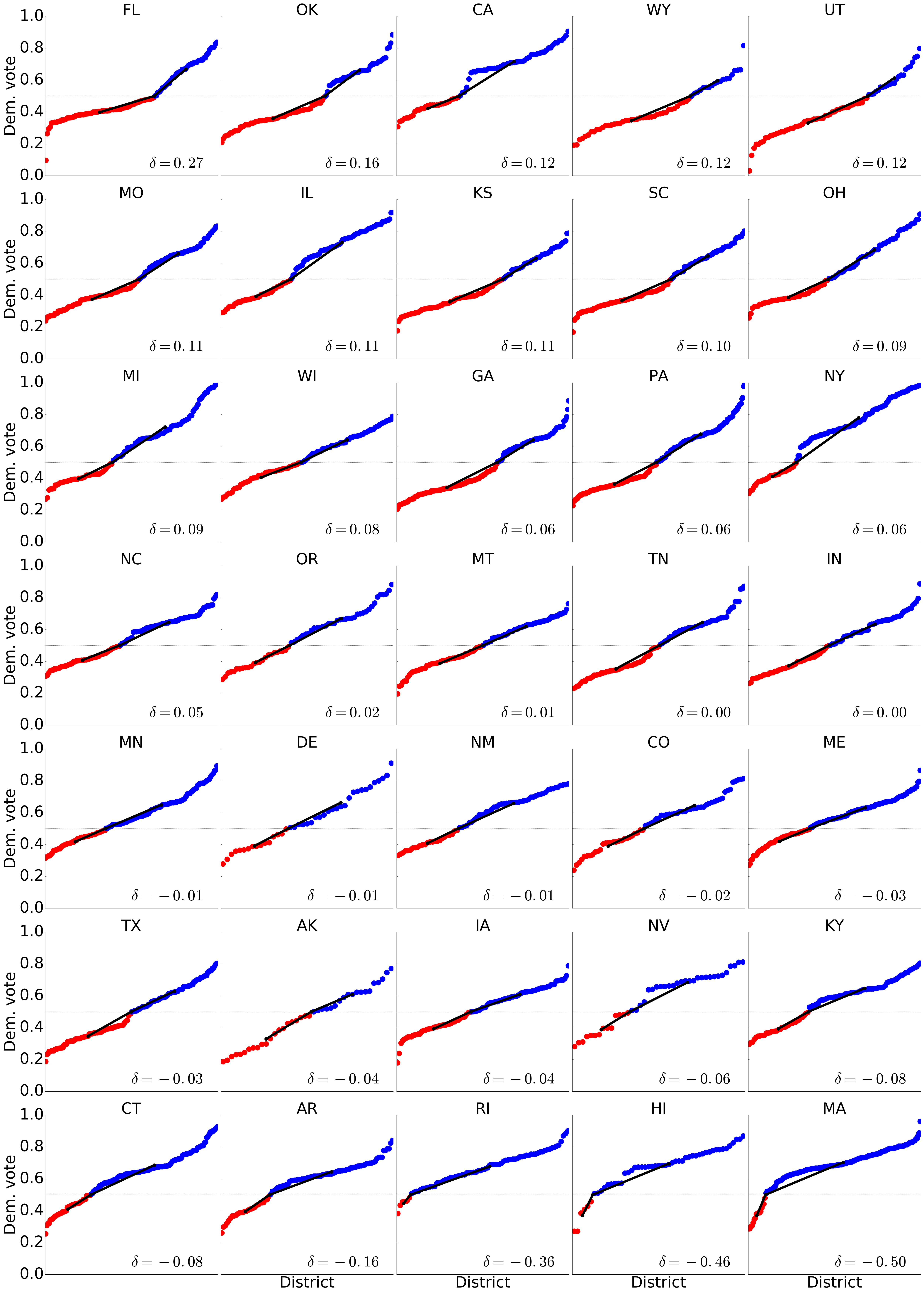 Figure 8
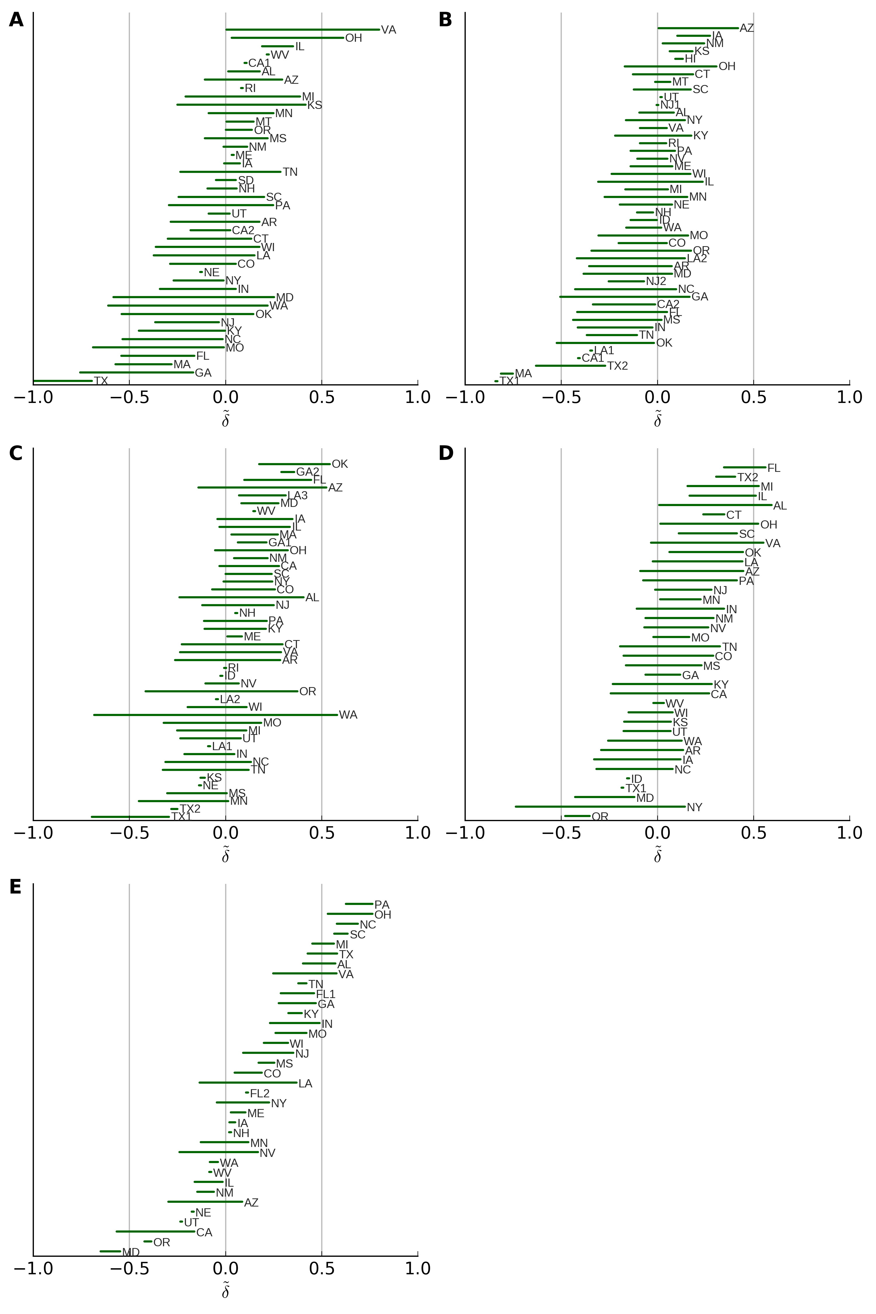 Figure 9
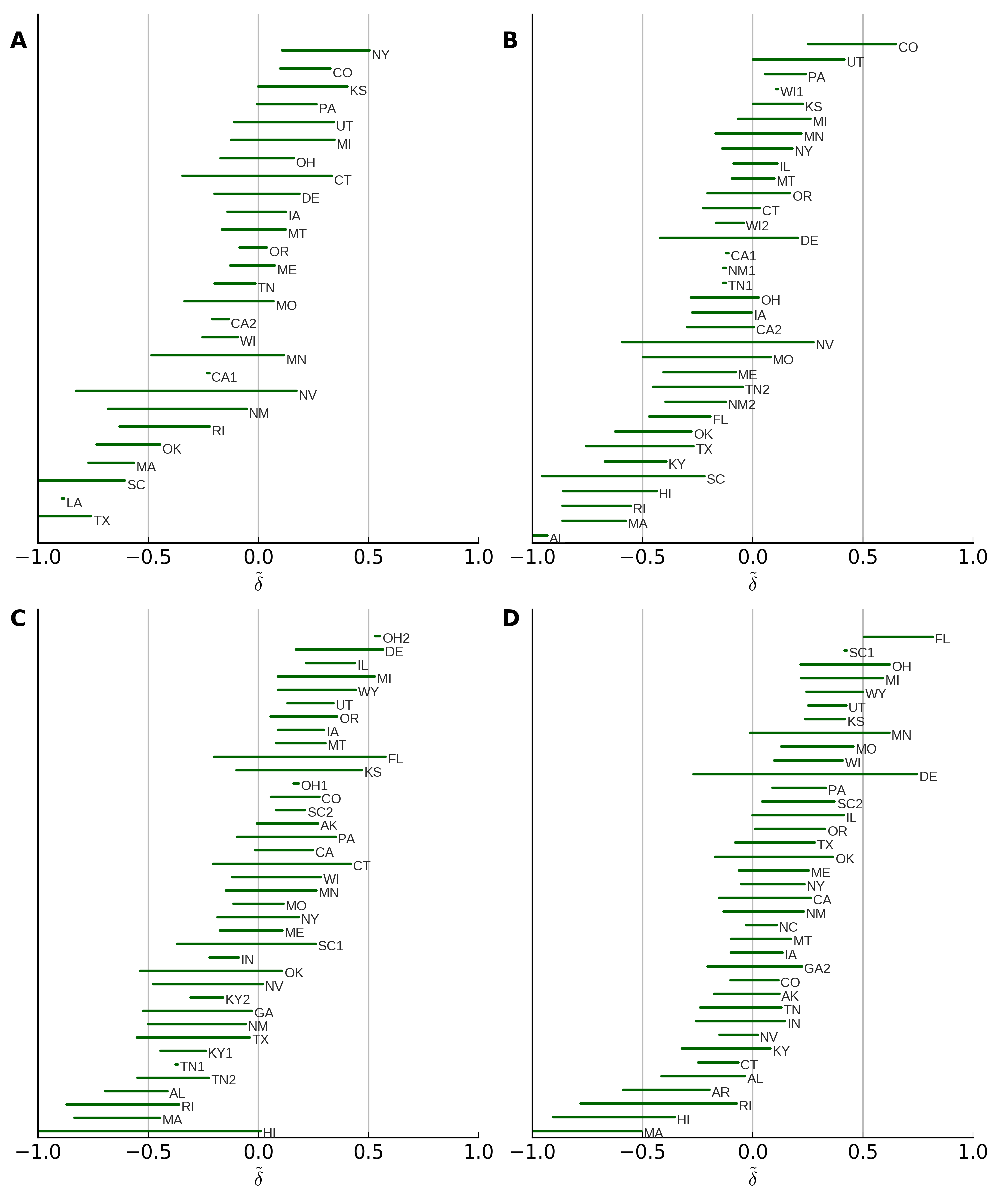 Figure 10
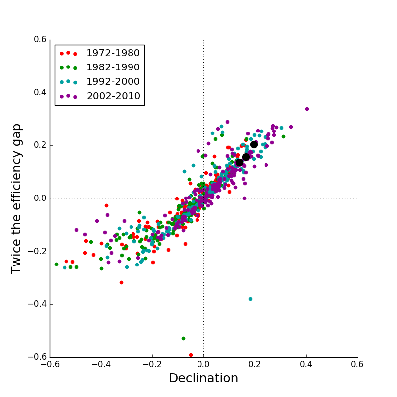 Figure 11
| State | No. Seats | Control | |||
|---|---|---|---|---|---|
| 0.76 | 0.53 | 4.8 | PA | 18 | R |
| 0.76 | 0.55 | 4.4 | OH | 16 | R |
| 0.58 | 0.48 | 2.6 | VA | 11 | R* |
| 0.58 | 0.45 | 2.9 | NC | 13 | R |
| 0.56 | 0.43 | 3.0 | MI | 14 | R |
| 0.49 | 0.44 | 2.0 | IN | 9 | R |
| 0.46 | 0.28 | 3.8 | FL | 27 | R |
| 0.44 | 0.24 | 4.4 | TX | 36 | R* |
| 0.42 | 0.40 | 1.6 | MO | 8 | R |
| 0.42 | 0.38 | 1.7 | TN | 9 | R |
| 0.35 | 0.28 | 1.7 | NJ | 12 | R |
| 0.32 | 0.31 | 1.2 | WI | 8 | R |
| 0.28 | 0.21 | 1.5 | GA | 14 | R |
| 0.16 | 0.09 | 1.3 | NY | 27 | S |
| 0.12 | 0.11 | 0.5 | MN | 8 | S |
| -0.08 | -0.07 | -0.3 | WA | 10 | S |
| -0.16 | -0.11 | -1.0 | IL | 18 | D |
| -0.19 | -0.10 | -2.6 | CA | 53 | D |
| -0.30 | -0.27 | -1.2 | AZ | 9 | S* |
| -0.55 | -0.53 | -2.1 | MD | 8 | D |
| Most positive | Most negative | |||||||||||
| Year | State | Seats | Year | State | Seats | |||||||
| 1980 | VA | 10 | 0.80 | 0.69 | 3.5 | 1976 | TX | 24 | -1.07 | -0.67 | -8.1 | |
| 2012 | PA | 18 | 0.76 | 0.53 | 4.7 | 1982 | TX | 27 | -0.83 | -0.51 | -6.8 | |
| 2012 | OH | 16 | 0.76 | 0.55 | 4.4 | 1990 | MA | 11 | -0.82 | -0.68 | -3.7 | |
| 2014 | NC | 13 | 0.69 | 0.54 | 3.5 | 1988 | MA | 11 | -0.79 | -0.66 | -3.6 | |
| 2016 | PA | 18 | 0.67 | 0.47 | 4.2 | 1984 | MA | 11 | -0.77 | -0.65 | -3.5 | |
| 2012 | SC | 7 | 0.63 | 0.65 | 2.3 | 1986 | MA | 11 | -0.77 | -0.64 | -3.5 | |
| 2014 | PA | 18 | 0.62 | 0.43 | 3.9 | 1972 | GA | 10 | -0.76 | -0.66 | -3.3 | |
| 2016 | NC | 13 | 0.61 | 0.48 | 3.1 | 1982 | MA | 11 | -0.75 | -0.63 | -3.5 | |
| 1972 | OH | 23 | 0.61 | 0.39 | 4.5 | 2008 | NY | 29 | -0.74 | -0.44 | -6.3 | |
| 2010 | AL | 7 | 0.59 | 0.61 | 2.1 | 1978 | TX | 24 | -0.73 | -0.46 | -5.5 | |
| 2014 | SC | 7 | 0.59 | 0.60 | 2.1 | 1980 | TX | 24 | -0.72 | -0.46 | -5.5 | |
| 1994 | WA | 9 | 0.58 | 0.53 | 2.4 | 1974 | TX | 24 | -0.71 | -0.45 | -5.4 | |
| 2016 | TX | 36 | 0.58 | 0.32 | 5.8 | 1972 | TX | 24 | -0.70 | -0.44 | -5.3 | |
| 2012 | NC | 13 | 0.58 | 0.45 | 2.9 | 1992 | TX | 30 | -0.70 | -0.41 | -6.1 | |
| 2012 | VA | 11 | 0.58 | 0.48 | 2.6 | 1972 | MO | 10 | -0.69 | -0.60 | -3.0 | |
| 1974 | OH | 23 | 0.57 | 0.37 | 4.2 | 1992 | WA | 9 | -0.68 | -0.62 | -2.8 | |
| 2012 | AL | 7 | 0.57 | 0.59 | 2.1 | 2014 | MD | 8 | -0.65 | -0.63 | -2.5 | |
| 2016 | SC | 7 | 0.56 | 0.58 | 2.0 | 1990 | TX | 27 | -0.63 | -0.38 | -5.2 | |
| 2012 | MI | 14 | 0.56 | 0.43 | 3.0 | 1978 | WA | 7 | -0.61 | -0.63 | -2.2 | |
| 2010 | FL | 25 | 0.56 | 0.35 | 4.4 | 1988 | TX | 27 | -0.60 | -0.36 | -4.9 | |
| 2002 | FL | 25 | 0.56 | 0.35 | 4.4 | 1994 | TX | 30 | -0.59 | -0.35 | -5.2 | |
| 2006 | VA | 11 | 0.55 | 0.46 | 2.5 | 1976 | WA | 7 | -0.59 | -0.60 | -2.1 | |
| 2016 | OH | 16 | 0.54 | 0.39 | 3.1 | 1980 | MD | 8 | -0.58 | -0.56 | -2.2 | |
| 1994 | OK | 6 | 0.54 | 0.60 | 1.8 | 2016 | MD | 8 | -0.58 | -0.56 | -2.2 | |
| 2014 | OH | 16 | 0.53 | 0.38 | 3.1 | 1980 | MA | 12 | -0.57 | -0.46 | -2.8 | |
| 2006 | MI | 15 | 0.53 | 0.39 | 2.9 | 2014 | CA | 53 | -0.57 | -0.29 | -7.6 | |
| 2004 | FL | 25 | 0.52 | 0.33 | 4.1 | 1974 | WA | 7 | -0.56 | -0.58 | -2.0 | |
| 2006 | OH | 18 | 0.52 | 0.36 | 3.3 | 2012 | MD | 8 | -0.55 | -0.53 | -2.1 | |
| 1998 | AZ | 6 | 0.52 | 0.58 | 1.8 | 1978 | FL | 15 | -0.54 | -0.40 | -3.0 | |
| 2000 | AZ | 6 | 0.51 | 0.57 | 1.7 | 1978 | OK | 6 | -0.54 | -0.60 | -1.8 | |
| 2010 | IL | 19 | 0.51 | 0.35 | 3.3 | 1978 | NC | 11 | -0.54 | -0.45 | -2.5 | |
| 2014 | MI | 14 | 0.50 | 0.38 | 2.7 | 1980 | OK | 6 | -0.54 | -0.60 | -1.8 | |
| 1972 | 1974 | 1976 | 1978 | 1980 | 1982 | 1984 | 1986 | 1988 | 1990 | 1992 | 1994 | 1996 | 1998 | 2000 | 2002 | 2004 | 2006 | 2008 | 2010 | 2012 | 2014 | 2016 | |
|---|---|---|---|---|---|---|---|---|---|---|---|---|---|---|---|---|---|---|---|---|---|---|---|
| AK | |||||||||||||||||||||||
| AL | 0.01 | 0.15 | 0.18 | 0.12 | 0.11 | 0.09 | 0.06 | -0.10 | -0.05 | 0.07 | 0.22 | -0.25 | 0.32 | 0.42 | 0.34 | 0.36 | 0.37 | 0.41 | -0.02 | 0.61 | 0.59 | 0.51 | 0.54 |
| AR | -0.45 | 0.33 | -0.23 | 0.06 | -0.09 | 0.11 | -0.51 | -0.38 | -0.36 | -0.40 | 0.41 | -0.10 | -0.17 | 0.01 | -0.38 | -0.42 | -0.24 | -0.21 | -0.27 | 0.19 | |||
| AZ | 0.39 | 0.42 | 0.05 | -0.16 | -0.11 | 0.01 | 0.41 | 0.52 | 0.45 | 0.42 | -0.16 | 0.48 | 0.52 | 0.58 | 0.57 | 0.36 | 0.43 | 0.05 | -0.09 | 0.07 | -0.28 | -0.35 | 0.01 |
| CA | 0.05 | 0.01 | -0.10 | -0.06 | -0.02 | -0.20 | -0.18 | -0.11 | -0.08 | -0.01 | 0.08 | 0.00 | 0.02 | 0.14 | -0.02 | -0.12 | -0.06 | 0.00 | 0.13 | -0.06 | -0.09 | -0.28 | -0.10 |
| CO | 0.06 | 0.01 | -0.33 | -0.24 | -0.36 | -0.10 | -0.04 | -0.23 | -0.01 | 0.05 | 0.28 | -0.08 | 0.04 | 0.08 | 0.20 | 0.30 | 0.17 | 0.14 | -0.18 | 0.09 | 0.19 | 0.05 | 0.11 |
| CT | -0.07 | 0.15 | -0.29 | -0.34 | -0.15 | -0.00 | -0.14 | 0.21 | -0.03 | -0.13 | -0.12 | -0.05 | 0.02 | -0.26 | 0.16 | 0.30 | 0.43 | 0.11 | |||||
| DE | |||||||||||||||||||||||
| FL | -0.35 | -0.14 | -0.12 | -0.40 | -0.25 | -0.00 | -0.28 | -0.13 | 0.02 | 0.03 | 0.06 | 0.09 | 0.20 | 0.22 | 0.28 | 0.29 | 0.35 | 0.29 | 0.19 | 0.29 | 0.27 | 0.15 | 0.06 |
| GA | -0.66 | -0.15 | -0.38 | -0.24 | -0.23 | -0.04 | -0.44 | 0.14 | 0.05 | 0.18 | 0.30 | 0.30 | 0.24 | 0.04 | -0.03 | -0.05 | 0.09 | 0.07 | 0.21 | 0.31 | 0.36 | ||
| HI | 0.27 | 0.38 | |||||||||||||||||||||
| IA | 0.07 | 0.02 | 0.08 | -0.01 | 0.06 | 0.11 | 0.19 | 0.21 | 0.30 | 0.26 | 0.43 | -0.05 | 0.25 | 0.43 | 0.14 | 0.15 | -0.22 | -0.11 | -0.41 | 0.07 | 0.03 | 0.06 | |
| ID | -0.40 | -0.27 | -0.01 | -0.05 | -0.43 | ||||||||||||||||||
| IL | 0.22 | 0.20 | 0.12 | 0.13 | 0.21 | 0.15 | -0.14 | -0.06 | -0.19 | -0.20 | 0.02 | -0.02 | 0.22 | 0.16 | 0.22 | 0.17 | 0.13 | 0.26 | 0.11 | 0.35 | -0.11 | -0.01 | -0.04 |
| IN | 0.04 | -0.29 | -0.23 | -0.11 | -0.07 | -0.02 | -0.10 | -0.15 | -0.10 | -0.36 | -0.19 | -0.12 | 0.04 | 0.01 | 0.04 | 0.05 | 0.31 | -0.10 | 0.01 | -0.02 | 0.44 | 0.21 | 0.31 |
| KS | 0.21 | 0.18 | -0.31 | 0.51 | 0.50 | 0.12 | 0.09 | 0.08 | 0.08 | 0.23 | -0.19 | -0.16 | -0.19 | -0.22 | -0.02 | -0.25 | 0.10 | ||||||
| KY | -0.47 | -0.01 | -0.13 | -0.01 | -0.02 | 0.19 | -0.07 | 0.03 | -0.22 | -0.16 | -0.12 | -0.12 | 0.23 | 0.09 | 0.18 | -0.11 | 0.31 | 0.04 | 0.16 | -0.26 | 0.44 | 0.38 | 0.36 |
| LA | -0.12 | 0.14 | -0.36 | -0.13 | -0.34 | -0.24 | -0.35 | 0.14 | 0.11 | 0.04 | 0.04 | -0.27 | 0.30 | 0.31 | 0.27 | -0.03 | 0.26 | 0.01 | 0.36 | 0.45 | 0.45 | 0.46 | 0.41 |
| MA | -0.21 | -0.41 | -0.34 | -0.43 | -0.48 | -0.63 | -0.65 | -0.64 | -0.66 | -0.68 | 0.03 | 0.05 | |||||||||||
| MD | 0.10 | 0.13 | 0.24 | -0.16 | -0.56 | -0.37 | -0.08 | 0.07 | -0.27 | -0.12 | 0.20 | 0.08 | 0.22 | 0.19 | 0.26 | -0.41 | -0.34 | -0.18 | -0.32 | -0.12 | -0.53 | -0.63 | -0.56 |
| ME | 0.12 | -0.40 | -0.06 | 0.22 | 0.24 | 0.02 | 0.29 | 0.08 | |||||||||||||||
| MI | 0.26 | 0.19 | 0.15 | -0.14 | -0.08 | -0.08 | -0.12 | 0.04 | -0.11 | -0.04 | -0.11 | -0.18 | -0.11 | -0.18 | 0.08 | 0.24 | 0.27 | 0.39 | 0.12 | 0.14 | 0.43 | 0.38 | 0.34 |
| MN | 0.16 | 0.09 | -0.09 | 0.00 | 0.24 | -0.02 | -0.11 | 0.15 | 0.07 | -0.26 | -0.28 | -0.44 | -0.25 | -0.33 | 0.01 | 0.08 | 0.15 | 0.01 | 0.21 | 0.09 | 0.11 | -0.12 | -0.09 |
| MO | -0.60 | -0.01 | -0.32 | -0.17 | -0.02 | 0.12 | -0.28 | 0.14 | 0.13 | 0.01 | -0.09 | -0.29 | 0.10 | -0.06 | 0.17 | 0.01 | -0.02 | 0.12 | 0.15 | 0.07 | 0.40 | 0.25 | 0.33 |
| MS | 0.27 | -0.14 | -0.10 | -0.05 | -0.02 | -0.05 | -0.14 | -0.55 | 0.02 | -0.38 | 0.01 | -0.07 | -0.17 | -0.04 | -0.12 | 0.11 | -0.24 | 0.33 | 0.36 | 0.25 | 0.33 | ||
| MT | 0.42 | 0.24 | 0.01 | 0.05 | 0.15 | 0.02 | 0.19 | 0.12 | -0.04 | ||||||||||||||
| NC | -0.16 | -0.05 | -0.16 | -0.45 | -0.01 | -0.36 | 0.08 | 0.06 | -0.32 | -0.09 | -0.25 | 0.07 | -0.13 | -0.02 | 0.10 | 0.02 | 0.06 | 0.02 | -0.06 | -0.25 | 0.45 | 0.54 | 0.48 |
| ND | |||||||||||||||||||||||
| NE | -0.23 | -0.24 | -0.36 | 0.13 | -0.24 | -0.30 | |||||||||||||||||
| NH | -0.28 | 0.16 | -0.10 | -0.07 | -0.31 | -0.07 | 0.17 | 0.08 | |||||||||||||||
| NJ | -0.03 | -0.18 | -0.27 | -0.11 | -0.04 | 0.00 | -0.08 | -0.05 | -0.15 | -0.19 | -0.10 | 0.20 | 0.15 | 0.05 | 0.10 | 0.05 | 0.09 | 0.22 | 0.06 | -0.01 | 0.28 | 0.17 | 0.07 |
| NM | 0.32 | 0.16 | -0.03 | 0.10 | 0.36 | 0.05 | 0.28 | 0.44 | 0.30 | 0.37 | 0.12 | 0.38 | 0.08 | 0.39 | 0.37 | 0.40 | 0.53 | -0.11 | -0.11 | -0.27 | -0.17 | ||
| NV | 0.00 | -0.31 | -0.08 | 0.14 | 0.01 | 0.20 | -0.27 | -0.31 | -0.13 | 0.27 | 0.48 | 0.01 | 0.28 | 0.06 | 0.24 | -0.35 | |||||||
| NY | -0.00 | -0.05 | -0.15 | -0.13 | -0.02 | 0.08 | -0.00 | 0.03 | -0.09 | -0.04 | 0.07 | 0.02 | 0.14 | 0.06 | -0.01 | -0.15 | -0.01 | 0.08 | -0.44 | -0.00 | 0.09 | -0.03 | 0.14 |
| OH | 0.39 | 0.37 | 0.12 | 0.11 | 0.02 | 0.20 | -0.11 | -0.04 | -0.02 | 0.04 | -0.04 | 0.22 | 0.08 | 0.14 | 0.14 | 0.23 | 0.31 | 0.36 | 0.01 | 0.28 | 0.55 | 0.38 | 0.39 |
| OK | -0.53 | 0.16 | -0.61 | -0.60 | -0.46 | -0.59 | -0.02 | -0.04 | -0.02 | 0.19 | 0.60 | 0.21 | 0.55 | 0.39 | 0.50 | 0.43 | 0.08 | ||||||
| OR | 0.00 | 0.20 | 0.17 | 0.05 | 0.03 | 0.22 | -0.43 | -0.41 | 0.12 | -0.39 | -0.39 | -0.52 | -0.53 | -0.55 | -0.46 | -0.44 | -0.60 | -0.48 | -0.51 | -0.53 | |||
| PA | -0.08 | 0.15 | -0.15 | -0.18 | -0.03 | -0.03 | -0.09 | 0.01 | -0.03 | 0.06 | -0.00 | -0.07 | 0.06 | -0.01 | 0.14 | 0.24 | 0.28 | 0.10 | -0.05 | 0.21 | 0.53 | 0.43 | 0.47 |
| RI | 0.26 | 0.13 | 0.01 | -0.27 | 0.09 | 0.00 | |||||||||||||||||
| SC | 0.01 | -0.24 | -0.27 | 0.10 | 0.22 | 0.05 | -0.01 | 0.19 | -0.06 | -0.14 | 0.07 | -0.00 | 0.13 | 0.27 | 0.24 | 0.12 | 0.17 | 0.13 | 0.31 | 0.46 | 0.65 | 0.60 | 0.58 |
| SD | 0.13 | -0.15 | 0.15 | ||||||||||||||||||||
| TN | 0.27 | -0.11 | -0.02 | -0.23 | -0.18 | -0.10 | -0.34 | -0.27 | -0.29 | -0.25 | -0.30 | -0.08 | 0.10 | 0.11 | 0.09 | -0.18 | -0.13 | -0.02 | -0.13 | 0.29 | 0.38 | 0.34 | 0.34 |
| TX | -0.44 | -0.45 | -0.67 | -0.46 | -0.46 | -0.47 | -0.20 | -0.14 | -0.37 | -0.39 | -0.41 | -0.35 | -0.17 | -0.19 | -0.16 | -0.20 | 0.22 | 0.18 | 0.23 | 0.20 | 0.24 | 0.24 | 0.32 |
| UT | 0.06 | -0.26 | 0.04 | 0.04 | 0.03 | -0.43 | 0.14 | -0.02 | -0.28 | -0.10 | 0.09 | 0.12 | -0.32 | -0.33 | |||||||||
| VA | 0.35 | 0.19 | 0.23 | -0.04 | 0.58 | -0.02 | -0.04 | 0.04 | -0.08 | -0.08 | -0.17 | -0.21 | -0.05 | -0.08 | 0.25 | 0.25 | 0.29 | 0.46 | -0.03 | 0.27 | 0.48 | 0.32 | 0.21 |
| VT | |||||||||||||||||||||||
| WA | 0.22 | -0.58 | -0.60 | -0.63 | -0.45 | -0.16 | -0.10 | 0.02 | -0.16 | -0.06 | -0.62 | 0.53 | 0.42 | -0.03 | -0.16 | -0.23 | 0.02 | 0.11 | -0.03 | -0.04 | -0.07 | -0.07 | -0.04 |
| WI | 0.16 | -0.15 | -0.33 | -0.19 | -0.05 | -0.01 | -0.22 | -0.12 | -0.16 | 0.16 | 0.10 | 0.00 | -0.18 | -0.02 | -0.18 | -0.07 | -0.09 | -0.15 | -0.14 | 0.07 | 0.31 | 0.19 | 0.20 |
| WV | 0.32 | 0.28 | -0.04 | 0.00 | 0.04 | 0.06 | 0.03 | -0.14 | |||||||||||||||
| WY |
| 1972 | 1974 | 1976 | 1978 | 1980 | 1982 | 1984 | 1986 | 1988 | 1990 | 1992 | 1994 | 1996 | 1998 | 2000 | 2002 | 2004 | 2006 | 2008 | 2010 | |
|---|---|---|---|---|---|---|---|---|---|---|---|---|---|---|---|---|---|---|---|---|
| AK | 0.00 | 0.01 | -0.02 | 0.03 | 0.13 | 0.06 | 0.09 | 0.05 | -0.06 | -0.16 | ||||||||||
| AL | -0.61 | -0.50 | -0.40 | -0.33 | -0.15 | -0.15 | -0.06 | 0.01 | ||||||||||||
| AR | -0.18 | -0.25 | -0.20 | -0.16 | -0.10 | |||||||||||||||
| AZ | ||||||||||||||||||||
| CA | -0.11 | -0.06 | -0.13 | -0.06 | -0.11 | -0.04 | -0.14 | -0.00 | -0.09 | 0.00 | 0.02 | 0.08 | 0.09 | 0.05 | -0.01 | -0.04 | -0.02 | 0.03 | 0.12 | -0.07 |
| CO | 0.06 | 0.11 | 0.11 | 0.13 | 0.07 | 0.13 | 0.30 | 0.13 | 0.11 | 0.16 | 0.03 | 0.06 | 0.11 | 0.13 | 0.11 | 0.06 | -0.04 | -0.04 | -0.02 | -0.05 |
| CT | 0.13 | -0.14 | -0.07 | -0.08 | -0.04 | 0.01 | -0.00 | -0.01 | -0.04 | -0.09 | 0.17 | -0.02 | -0.04 | -0.08 | -0.05 | -0.02 | -0.07 | -0.03 | -0.07 | -0.10 |
| DE | 0.04 | -0.02 | -0.11 | 0.02 | 0.10 | -0.23 | 0.01 | -0.01 | -0.06 | 0.08 | 0.06 | 0.17 | 0.19 | 0.22 | 0.29 | 0.40 | 0.29 | 0.27 | -0.00 | -0.14 |
| FL | -0.16 | -0.20 | -0.12 | -0.14 | -0.08 | -0.07 | -0.10 | 0.03 | 0.16 | 0.25 | 0.26 | 0.34 | 0.27 | 0.26 | 0.21 | |||||
| GA | -0.19 | -0.18 | -0.06 | -0.02 | -0.04 | -0.06 | 0.07 | 0.05 | -0.05 | |||||||||||
| HI | -0.32 | -0.22 | -0.25 | -0.43 | -0.29 | -0.66 | -0.54 | -0.30 | -0.25 | 0.01 | -0.18 | -0.37 | -0.31 | -0.46 | -0.38 | |||||
| IA | 0.05 | -0.02 | -0.06 | 0.02 | 0.05 | -0.06 | -0.12 | -0.04 | -0.08 | -0.01 | 0.06 | 0.10 | 0.04 | 0.11 | 0.13 | 0.04 | 0.02 | 0.05 | -0.05 | -0.02 |
| ID | ||||||||||||||||||||
| IL | -0.01 | -0.04 | 0.05 | -0.00 | -0.02 | 0.08 | 0.15 | 0.19 | 0.15 | 0.14 | 0.06 | 0.11 | 0.17 | 0.11 | 0.00 | |||||
| IN | -0.10 | -0.06 | -0.04 | -0.07 | -0.07 | -0.12 | -0.04 | 0.06 | -0.01 | 0.01 | ||||||||||
| KS | 0.13 | 0.17 | 0.04 | 0.06 | -0.00 | 0.09 | 0.07 | 0.10 | -0.00 | -0.02 | -0.04 | -0.01 | 0.00 | 0.09 | 0.18 | 0.10 | 0.14 | 0.20 | 0.11 | 0.14 |
| KY | -0.30 | -0.20 | -0.26 | -0.17 | -0.19 | -0.15 | -0.11 | -0.10 | -0.11 | -0.13 | -0.06 | 0.02 | -0.09 | -0.14 | ||||||
| LA | -0.36 | |||||||||||||||||||
| MA | -0.19 | -0.26 | -0.26 | -0.28 | -0.34 | -0.32 | -0.29 | -0.33 | -0.23 | -0.17 | -0.27 | -0.29 | -0.24 | -0.33 | -0.37 | -0.41 | -0.37 | -0.50 | -0.20 | |
| MD | ||||||||||||||||||||
| ME | 0.02 | -0.04 | -0.03 | -0.05 | -0.08 | -0.16 | -0.06 | -0.02 | 0.00 | 0.04 | 0.04 | -0.07 | 0.01 | 0.10 | 0.03 | -0.03 | -0.02 | |||
| MI | -0.02 | 0.15 | 0.01 | -0.05 | -0.03 | 0.11 | -0.03 | 0.03 | -0.01 | 0.05 | 0.15 | 0.04 | 0.10 | 0.17 | 0.22 | 0.25 | 0.20 | 0.21 | 0.09 | 0.19 |
| MN | -0.20 | -0.19 | 0.04 | 0.01 | 0.02 | 0.09 | -0.07 | -0.06 | -0.02 | -0.05 | -0.06 | 0.06 | 0.07 | 0.11 | 0.25 | 0.15 | 0.02 | -0.01 | 0.13 | |
| MO | 0.02 | -0.02 | -0.11 | -0.13 | -0.10 | -0.19 | -0.18 | 0.04 | -0.04 | -0.04 | 0.02 | 0.01 | 0.05 | 0.06 | 0.14 | 0.17 | 0.09 | 0.09 | ||
| MS | ||||||||||||||||||||
| MT | -0.08 | -0.02 | -0.03 | 0.05 | -0.03 | -0.04 | 0.04 | 0.02 | -0.03 | 0.06 | 0.09 | 0.13 | 0.09 | 0.02 | 0.03 | -0.04 | 0.02 | 0.01 | 0.07 | |
| NC | 0.04 | -0.00 | 0.02 | 0.01 | -0.00 | |||||||||||||||
| ND | ||||||||||||||||||||
| NE | ||||||||||||||||||||
| NH | ||||||||||||||||||||
| NJ | ||||||||||||||||||||
| NM | -0.32 | -0.16 | -0.17 | -0.02 | -0.15 | -0.06 | -0.08 | -0.16 | -0.08 | -0.20 | -0.23 | -0.17 | -0.03 | -0.01 | -0.08 | -0.09 | 0.02 | 0.10 | -0.01 | 0.05 |
| NV | 0.09 | -0.24 | -0.47 | 0.05 | -0.13 | 0.03 | 0.15 | -0.25 | -0.32 | -0.00 | -0.26 | 0.01 | -0.12 | -0.24 | -0.21 | 0.01 | -0.07 | -0.01 | -0.06 | -0.08 |
| NY | 0.20 | 0.15 | 0.10 | 0.08 | 0.04 | -0.00 | -0.06 | 0.05 | -0.01 | 0.07 | -0.05 | -0.06 | 0.08 | 0.04 | 0.07 | -0.01 | 0.02 | 0.09 | 0.05 | 0.00 |
| OH | -0.04 | 0.07 | -0.02 | -0.08 | -0.06 | 0.01 | -0.12 | -0.07 | -0.10 | -0.05 | 0.06 | 0.08 | 0.24 | 0.24 | 0.23 | 0.25 | 0.25 | 0.27 | 0.09 | 0.14 |
| OK | -0.19 | -0.21 | -0.32 | -0.23 | -0.24 | -0.27 | -0.24 | -0.18 | -0.19 | -0.11 | -0.22 | -0.24 | -0.21 | -0.10 | 0.05 | -0.08 | 0.06 | 0.14 | 0.16 | 0.16 |
| OR | 0.02 | -0.03 | -0.03 | -0.04 | -0.02 | -0.10 | -0.10 | 0.01 | -0.01 | 0.08 | 0.11 | 0.03 | 0.08 | 0.17 | 0.13 | 0.16 | 0.16 | 0.11 | 0.02 | 0.01 |
| PA | 0.02 | 0.10 | -0.00 | 0.05 | 0.02 | 0.09 | 0.02 | 0.05 | 0.02 | 0.04 | 0.06 | -0.03 | 0.08 | 0.07 | 0.13 | 0.05 | 0.13 | 0.12 | 0.06 | 0.03 |
| RI | -0.10 | -0.10 | -0.22 | -0.27 | -0.18 | -0.32 | -0.23 | -0.26 | -0.28 | -0.38 | -0.16 | -0.38 | -0.25 | -0.37 | -0.23 | -0.36 | -0.16 | -0.04 | -0.35 | -0.33 |
| SC | -0.26 | -0.46 | -0.39 | -0.43 | -0.36 | -0.40 | -0.19 | -0.18 | -0.09 | -0.14 | -0.09 | 0.09 | 0.06 | 0.08 | 0.13 | 0.08 | 0.13 | 0.11 | 0.05 | |
| SD | ||||||||||||||||||||
| TN | -0.01 | -0.01 | -0.08 | -0.02 | -0.08 | -0.06 | -0.17 | -0.04 | -0.04 | 0.00 | -0.18 | -0.25 | -0.16 | -0.12 | -0.10 | -0.10 | -0.08 | 0.01 | 0.01 | 0.11 |
| TX | -0.53 | -0.52 | -0.31 | -0.30 | -0.22 | -0.11 | -0.10 | -0.11 | -0.15 | -0.24 | -0.07 | -0.03 | -0.01 | 0.07 | 0.02 | 0.05 | -0.06 | 0.05 | ||
| UT | 0.01 | 0.04 | -0.05 | 0.10 | 0.12 | 0.16 | 0.21 | 0.11 | 0.01 | 0.03 | 0.05 | 0.06 | 0.15 | 0.15 | 0.08 | 0.12 | 0.16 | 0.20 | 0.11 | 0.15 |
| VA | ||||||||||||||||||||
| VT | ||||||||||||||||||||
| WA | ||||||||||||||||||||
| WI | -0.11 | -0.07 | -0.08 | -0.09 | -0.08 | 0.05 | -0.02 | -0.04 | -0.02 | -0.07 | 0.00 | -0.05 | 0.01 | 0.10 | 0.13 | 0.10 | 0.17 | 0.14 | 0.08 | 0.03 |
| WV | ||||||||||||||||||||
| WY | 0.18 | 0.11 | 0.05 | 0.14 | 0.23 | 0.14 | 0.18 | 0.18 | 0.06 | 0.26 |
Peer Reviews
No public reviews on file for this paper yet. If you reviewed it on a platform where reviews are public (OpenReview, ICLR, NeurIPS, ICML), you can paste yours below so the community can read it here.
Videos
No videos yet. Explain this paper in a talk, walkthrough, or lecture? Add one.
Quantifying gerrymandering using the vote distribution
Gregory S. Warrington1∗
1Department of Mathematics & Statistics, University of Vermont,
16 Colchester Ave., Burlington, VT 05401, USA
∗To whom correspondence should be addressed; E-mail: [email protected]
(May 15, 2017)
Abstract
To assess the presence of gerrymandering, one can consider the shapes of districts or the distribution of votes. The efficiency gap, which does the latter, plays a central role in a 2016 federal court case on the constitutionality of Wisconsin’s state legislative district plan. Unfortunately, however, the efficiency gap reduces to proportional representation, an expectation that is not a constitutional right. We present a new measure of partisan asymmetry that does not rely on the shapes of districts, is simple to compute, is provably related to the “packing and cracking” integral to gerrymandering, and that avoids the constitutionality issue presented by the efficiency gap. In addition, we introduce a generalization of the efficiency gap that also avoids the equivalency to proportional representation. We apply the first function to US congressional and state legislative plans from recent decades to identify candidate gerrymanders.
1 Introduction
To gerrymander is to intentionally choose voting districts so as to actively (dis)advantage one or more groups111There is no universally agreed upon definition. In particular, usage in the courts differs from colloquial usage.. While gerrymandering can focus on various types of groups, such as incumbents or those formed by shared race, our focus in this article is the case in which the disadvantaged group is a political party, that is, partisan gerrymandering.
Approaches towards preventing gerrymanders include vesting the responsibility of drawing districts in non-partisan commissions (see [Win08]); drawing districts by putatively neutral algorithms (such as the shortest splitline method [KYS07]); or moving away from the current district-based single member plurality system (see [Gro81] for various alternatives). Since efforts along these lines have not yet eradicated gerrymandering, there is a need for methods that can accurately identify any gerrymanders that do occur.
Historically, gerrymanders have been identified by unusual district boundaries [Gri]. In fact, it was the resemblance of a Massachusetts senatorial district to a salamander that gives gerrymandering its name (Elbridge Gerry signed off on the district in 1812 while governor of Massachusetts). To this day, unexpected shapes of districts lead to both zoomorphic comparisons (e.g., Pennsylvania’s 6th congressional “dragon” district) and allegations of gerrymandering.
In response, a number of researchers have created compactness metrics as a way to help identify gerrymandered districts (see [NGCH90] for an overview); a recent, related Markov-chain based approach is found in [CFP17]. While such approaches are important tools, the fact that partisan asymmetries arise naturally from “human geography” [CR13] strongly suggests gerrymanders can exist without contorted boundaries. By analogy, just as one can be ill and yet not have a fever, so can one have a gerrymander without violating compactness.
For more than four decades, vote-distribution asymmetries have been analyzed via the “seat-votes curve” (see, for example, [Tuf73, GK94, KGC08, Nag15]), the computation of which requires significant statistical assumptions. In 2014, McGhee [McG14] introduced an alternative, the efficiency gap (see also [MS15]). This function is easily computed from its elegant definition without any assumptions at all when all races are contested. A short derivation (see [McG14] or the derivation of equation (6)) shows that a fair district plan according to the efficiency gap is one in which the seats won and the vote won are proportional with constant : Winning (that is, ) of the vote will earn (that is, ) of the seats when the efficiency gap is zero.
As detailed in [MS15, III.C], several decades of court cases predicated on partisan gerrymandering have, until recently, been uniformly unsuccessful in the federal courts: On November 21, 2016, a three-member circuit court panel ruled in Whitford v. Gill [Wis] that the districts drawn for the Wisconsin lower house are an unconstitutional partisan gerrymander. This is the first time such a determination has been made regarding an alleged partisan gerrymander [Win16]. A significant part of the panel’s decision relies on the supporting evidence of asymmetry afforded by the efficiency gap. However, in his dissent in Whitford v. Gill, Chief Judge Griesbach objects to the reliance on the efficiency gap, in large part on the grounds that the US Supreme Court has ruled that there is no constitutional right to proportional representation [Vie]. A natural question is whether there are alternative functions that do not reduce to proportional representation.
Below we do define a family of functions, indexed by nonnegative numbers , that specializes to (twice) the efficiency gap when . As we’ll describe in Section 4, for these functions do not reduce to proportionality. However, the focus in this article will be on a new function for identifying gerrymandering we term the declination. It is a measure of asymmetry in the vote distribution that relies only on the fraction of seats each party wins in conjunction with the aggregate vote each party uses to win those seats. (The declination is essentially an angle associated to the vote distribution; its name is in analogy with the angular difference between true north and magnetic north.) The declination does not require the significant statistical assumptions required to compute the seats-votes curve nor the proportional-representation assumption embedded in the efficiency gap.
To be useful for identifying gerrymanders, our functions must measure asymmetry that arises from gerrymandering rather than from other sources. Asymmetries that are caused by partisan gerrymandering arise from two primary techniques. The first is to pack certain districts with members of party so that party wins those districts overwhelmingly, thereby wasting votes that could have been helpful in winning districts elsewhere. A second technique, naturally paired with the first, is to crack the party- voters by distributing them among districts so as to prevent them from having sufficient power to win elections outside of the packed districts. Overall, party wins a small number of overwhelming victories while suffering a large number of narrow losses. In Theorem 1 we rigorously prove that the declination increases in response to packing and cracking.
In Section 2 we define the declination and two variations. Analyses of elections in recent decades using the declination are presented in Section 3. The -gap family of functions that generalizes the efficiency gap is introduced in Section 4. In Section 5 we formally present the theorem showing that both the declination and the -gap increase in response to packing and cracking. In Section 6 we discuss the relative merits of the declination, the -gap, the efficiency gap and the mean-median. In Section 7 we outline the data sets used as well as the statistical model used to impute votes in uncontested elections. We conclude in Section 8. Additional figures and tables are included in the appendix.
2 The declination
Our definition of the declination stems from the observation that in a randomly chosen (i.e., ungerrymandered) district plan, the threshold for the fraction of democratic votes in a district does not play a distinguished role. Quirks of geography and sociology will certainly shape the distribution in various ways that we will not attempt to model. But we expect a phase shift across the threshold no more than we would expect one across or . Partisan gerrymandering, almost by definition, modifies a natural distribution in a manner that treats the threshold as special. Accordingly, one approach to recognizing gerrymanders is to contrast the set of values below with the set of values above .
In order to compare these two parts of the vote distribution, we introduce some notation: Define an election with districts to be a triple consisting of political parties and along with a vector that records the fraction of the two-party vote won by party in each of the districts. We assume, without loss of generality, that our districts are ordered in increasing order of party- vote share:
[TABLE]
Set and let and . Let and be the centers of mass of the points in and , respectively (we therefore assume that ). Set , and ; see Fig. 1. In a district plan in which neither side has an inherent advantage, we would expect the point to lie on the line . Deviation of above is indicative of an advantage for party while deviation below is indicative of an advantage for party . This suggests, as a measure of partisan asymmetry, the declination, , where
[TABLE]
Dividing by converts from radians to fractions of degrees; possible values of the declination are between and .
To each party we are associating a line whose direction encodes the average vote the party gets in the districts it wins along with the total number of districts it wins. When a party uses lots of extra votes to win few districts, the slope of this line is high. The declination, up to the -scaling, is the angle between the lines associated to the two parties.
Fig. 2 illustrates how the declination and the efficiency gap evaluate different elections differently. In this figure and the remainder of the article, we identify Party with the Democrats and Party with the Republicans. As a result, positive values of the declination are favorable to Republicans.
As illustrated in Figure 3.A, packing or cracking a single district leads to a change of approximately in the declination. Hence, as a measure of the number of seats affected by the partisan advantage, we also consider .
As a second variation, the value of has minimal correlation with (see Fig. 3.B) and hence is useful when comparing the declinations of elections with different numbers of districts.
3 Analyses of elections
Fig. 4 displays the distribution of values over time for state legislative (lower house) and congressional races going back to 1972 (see Section 7 for a detailed description of the data used). We prove in Theorem 1 that the declination increases (resp., decreases) as a result of gerrymandering engendered by packing and cracking by party (resp., party ).
There is no gold standard for assessing gerrymandering. As a result, there is no direct way to validate the declination as a measure of gerrymandering. However, we can still review the extent to which the declination agrees with other measures of gerrymandering. Table 1 lists the values of , and for congressional races in 2012. There is marked consistency between the declination and who controlled the redistricting process subsequent to the 2010 census. Also, while disproportionality may not be sufficient evidence to denounce a district plan as an unconstitutional gerrymander, a successful gerrymander by definition results in one party winning fewer seats than it would under a neutral plan. This is consistent with what happened in the first four states in Table 1 (Pennsylvania, Ohio, Virginia and North Carolina): As noted in [Wan16], the Democrats earned approximately half the statewide vote in 2012 in each of these states while garnering no more than 31% of the seats in any of the four.
There is also strong agreement between the declination and compactness metrics (we work here with ; and are similarly concurrent). In [Ing14], each 2012 congressional district is scored by the Polsby-Popper compactness metric (scaled to run from 0 to 100; higher scores indicate less compact). The nine states with at least eight districts and at least one district scoring greater than 90 are North Carolina, Ohio, Pennsylvania, Virginia (the first four listed in Table 1); California, Illinois and Maryland (three of the last four in Table 1); as well as Florida and Texas. Intriguingly, the declination identifies Indiana as a likely gerrymander, in contrast to its evaluation in [Ing14] as a state with very compact districts.
The matter of determining a standard for what qualifies as an unconstitutional partisan gerrymander is beyond the scope of this article. (See [MS15] for a comprehensive treatment utilizing the efficiency gap, [MSK15] for the seats-votes curve and [MB15, Wan16] for the mean-median difference.) In addition to the nontrivial task of addressing guidance from the courts, two significant issues that must be addressed are the reality that any measure of asymmetry in vote distributions will vary from election to election (see Fig. 5) and that there may be an inherent partisan asymmetry due to how voters are distributed geographically. We briefly address each issue.
We consider the first problem by determining how large the declination must be in absolute value before we are confident that it will not equal zero for a different election in the same ten-year districting cycle. Figs. 10 and 11 illustrate the total range of values for each state in each redistricting cycle. With respect to our historical data set of 1 195 elections included in these figures, for over eighty percent of the elections with , the declination (i.e., the partisan advantage) persists in sign over the course of the entire ten-year redistricting cycle in which lies. With this confidence, therefore, we conclude from Table 1 (without examining data from 2014 or 2016) that the partisan advantage for the congressional district plans in Pennsylvania, Ohio, Virginia, North Carolina, Michigan, Indiana and Maryland are likely to persist through 2020. We note that the 2012 Wisconsin legislative election, with , just meets this threshold (also see Fig. 6). For reference, the most extreme values of the declination for congressional races since 1972 are sorted in Table 2.
The second major issue, inherent partisan advantages arising from how voters are distributed geographically, is an important one. As explored in [CR13], such realities may lead to one party naturally garnering more than 55% of the seats with only 50% of the vote. For example, if we take the republican advantage in Pennsylvania to be 8% (following [CR13]), this seat advantage translates into a value of of approximately . Since for the 2012 Pennsylvania congressional election, we can still conclude with high confidence that the partisan advantage for the Republicans beyond any geographic advantage will persist through 2020. Ultimately, the proper way to account for any inherent geographic advantages requires answering the following: To what extent is it constitutional for a district plan to exacerbate (or mitigate) existing, natural advantages?
Additional summary tables and figures are included in the appendix. Specifically, Tables 3 and 4 list the declination for all 1142 congressional elections and 646 state legislative elections in the data set. Figs. 8 and 9 depict the actual vote distributions (utilizing imputed vote values for uncontested races (see Section 7) along with the declination for the 2016 congressional elections and the 2008 state legislative elections, respectively.
4 A generalization of the efficiency gap
In this section we introduce a variation on the efficiency gap function. We first review the definition of the efficiency gap before generalizing it in the next subsection.
McGhee defines a vote as wasted if either 1) it is a vote for the winning candidate in excess of the one-more-than-50% needed to win the election or 2) it is a vote for the losing candidate. The motivation for this definition is that packing and cracking produce more wasted votes in won and lost districts, respectively. In light of this, the difference in the total number of votes wasted by each party should reflect the extent to which the packing and cracking treats the parties asymmetrically.
Given an election , party ’s waste in district , , is in those districts it wins and in those districts it loses. Party ’s waste is .
McGhee [McG14, Eq. (2)] (using different notation and terminology) made the following definition: The efficiency gap of is
[TABLE]
A positive (resp., negative) efficiency gap indicates that party (resp., ) is wasting more votes. As such, “fair” district plans should have efficiency gaps close to zero.
4.1 The function
The efficiency gap takes a binary view of votes: Either a vote contributes to the first 50% required for a candidate’s win, and is therefore not wasted at all, or it doesn’t contribute, and is therefore completely wasted. We now explore a more general paradigm in which there is a continuum of waste that is shaped by a parameter .
As motivation for this generalization, consider the party- gerrymanderers. They are not aiming to have the party- candidates win districts by exactly one vote above 50%. To do so would skirt disaster. If their projections are even slightly too optimistic, then the gerrymander will backfire spectacularly with each chosen candidate losing by a razor-thin margin. It is less reckless for party to aim for comfortable margins in each district they aim to win. Consequently, it is reasonable to consider the votes just above 50% as only partially wasted while treating any votes near 100% as almost fully wasted.
For simplicity, we view the votes won by a given candidate as ordered. For a winning candidate, the first half of the votes in the district contribute directly to the win. The subsequent votes for the winner, and all votes for the loser, are assigned waste values determined by the parameter . As will become apparent, setting corresponds to weighting all wasted votes the same amount.
Given an -district election , for each , , set . When is positive, party wins district and is the fraction of the wasted votes that are wasted by . When is negative, party wins district and measures the fraction of wasted votes wasted by party . For any nonnegative real number and any , we define the -waste of party in district to be
[TABLE]
For , similarly define . The remaining values are determined by requiring that the total waste in each district , , is constant and equal to . Set and . Finally, define the -gap of election to be
[TABLE]
Note that for any election , is twice the efficienct gap.
We now derive a formula for the -gap that expresses it in terms of the . First we note that
[TABLE]
Second, . Plugging into equation (5), we find that
[TABLE]
It follows that
[TABLE]
where for and for .
We see that precisely when
[TABLE]
Let denote the overall vote fraction won by party . Rewriting (7), we find that the efficiency gap being zero is equivalent to . We have recovered the observation of [McG14, MS15] that the efficiency gap is zero exactly when the excess in fraction of seats won above one half is twice the excess in vote fraction above one half.
For general , however, the relationship between seats won and votes earned in an election for which is zero is more complicated and depends on how the votes are distributed. When is a nonnegative even integer of the form , we can express the condition succinctly since then
[TABLE]
where denotes the th moment of the .
In the limit as , reduces (in the general case of for all ) to . It follows that is zero if and only if each party wins half of the seats, irrespective of overall vote share.
There are at least two natural ways in which the -gap could be further generalized. The first is by allowing the waste to be most pronounced close to the 50% threshold. This is conveniently attained by considering waste functions of the form for . This choice has several appealing characteristics such as the fact that the winner and loser waste equal amounts more evenly than the 75%-25% split for the efficiency gap. In addition, the waste function is more sensitive to what is happening near the 50% threshold. Unfortunately, this latter property seems to reduce its utility greatly as there is much more noise due to random fluctuations in vote earned.
Second, while we have restricted our attention to power functions determined by a parameter , the concept of -waste could easily be extended to more sophisticated functions. One could also allow different functions for the votes wasted by the winner and the votes wasted by the loser.
5 Theorem on packing and cracking
We make precise the link between packing and cracking and the functions we introduce in the previous two sections. Define -cracking to be the moving of party- votes from district to districts such that 1) the first districts are still lost by party after the redistribution and 2) district becomes a district that party loses. Similarly, define -packing to be the moving of party- votes from district to districts such that district is now lost by party . Using our new terminology, we state and prove the following
Theorem 1. Let be an election with in weakly increasing order. Let be the average party- vote in the districts lost by party and be the corresponding average in the districts won by party . Let be the party- vote fraction remaining in district after -cracking or -packing and the resulting election.
If , then . 2. 2.
If , then .
Proof.
Proof of (1). We refer the reader to Fig. 1 for the positions of points referenced. The -packing or -cracking of district will move point to the right by units. Each of points and will move to the right by only units. Since , point will also move up. Since is arranged in increasing order, point will also move up. Together, these shifts will decrease and increase , thereby increasing . By symmetry, -packing and -cracking will decrease .
Proof of (2). We show only the details for -cracking; the argument for -packing is similar. Let be the vote distribution for . Since we are -cracking the st district, we know that for . Set for . Note in the below equations that all and for are negative ( is negative as well). Recall that
[TABLE]
We wish to show that the difference
[TABLE]
is positive. Multiplying by , we see that this is equivalent to showing that
[TABLE]
We make the following observations. First, since all votes being moved are going from district to a district with , we must have . Second, since is positive . So choose constants such that for . Straightforward calculus shows that, since is an increasing function and for all by hypothesis, that for all . It follows that
[TABLE]
As , the result follows. ∎
6 Strengths and weaknesses of different functions
Our situation in identifying gerrymanders is analogous to that of assessing intelligence. Emotional intelligence and logical intelligence are best measured by different types of questions; no single question type can capture the spectrum of ways in which intelligence can manifest itself. Every test for gerrymandering will have its strengths and weaknesses. In this section we attempt to illustrate, through concrete examples, ways in which each of the efficiency gap, the -gap, the mean-median difference and the declination can give misleading answers in their attempts to identify gerrymanders.
The oldest tool for this purpose, the seats-votes curve, has been around for over 40 years [Tuf73]. Notwithstanding its theoretical interest and applications in such areas as predictions (for example, [KGC08]), as it has not led to a manageable judicial standard for gerrymandering in this span, we will not address it directly in the remainder of this article.
6.1 The efficiency gap
The efficiency gap, through its role in Whitford v. Gill, has already proven its utility. And while its simplicity is an asset, it also has several drawbacks. First, by requiring that there be proportional representation for an election to be considered fair, it conflicts with constitutional law [Vie]. Second, it is simple to construct hypothetical examples for which a natural district plan leads to a constant of proportionality different from (see, for example, Figs. 2.C,D). While the proportionality asserted by the efficiency gap may hold in some overall sense, for the instances for which it doesn’t we are left in the difficult position of determining whether any deviation from this average law is due to gerrymandering or natural deviation. And, as illustrated by our definition of the -gap function, the proportionality with a constant of depends on a subjective decision on how to weight various wasted votes. Third, there are historical examples in which the proportionality holds, but the shape of the vote distribution suggests significant partisan asymmetry (see, in particular, the 1974 Texas congressional election shown in Fig. 2.A as well as the 2012–2016 Tennessee congressional elections, the last of which is displayed in Fig. 8).
6.2 The -gap
The -gap family of functions is appealing due to its close connection to the efficiency gap and the fact that it does not reduce to proportionality. Additionally, when , the -gap is closely related to skewness of the -distribution (see (8)), a standard measure of symmetry in statistical distributions. We also note that when , the correlation between the declination and the -gap is very high ( among congressional elections). Unfortunately, the -gap family has its own drawbacks.
First, there is no reason to think that one value of will prove superior to other values in all cases. For example, consider the 1974 Texas and North Carolina congressional elections (see Fig. 2.A and Fig. 7.A, respectively). Proportionality is essentially met in both cases as reflected by the values of being close to zero; each election is fair according to the efficiency gap. In contrast, is approximately for each, indicating strong asymmetry. While we have no absolute way of determining whether one or both is a gerrymander, evidence suggests that makes the correct assessment for the North Carolina election (little or no gerrymandering) while makes the correct assessment for the Texas election (gerrymandering)222As described in [O’C90, pg. 35], there was not significant partisan rancor during the 1971 redistricting and the Democrats received approximately 63% of the congressional vote while winning 82% (9 of 11) congressional seats. Of course, these facts have little bearing on whether there may have been racial gerrymandering. For the Texas election, one author [May71] suggests that for the 1965 redistricting, protecting incumbents was a higher priority than advantaging the Democrats as a party. The constructions of a large number of safe seats for incumbents would certainly be consistent with the distribution seen.. We note that the declination yields what we believe to be the correct answer in both cases.
Second, even if there were one value of that was superior to all others, it is unclear what theoretical, rather empirical, justification could be used to support it. Third, as shown by (6), the -gap is essentially an interpolation, albeit a complicated one, between the proportionality with constant , when , and proportionality with constant [math], when . (A fair election for the latter is one in which each party gets half the seats, regardless of the fraction of votes won by each side.)
6.3 The mean-median difference
The difference between the mean and the median of the democratic vote fraction among all districts has been suggested as yet another way of measuring partisan asymmetry (see, for example, Wang [Wan16] and [KMM*+*16, MB15]). A large difference between these values can indeed accompany an asymmetry in the vote distribution. For example, in the 2012 Pennsylvania congressional election (see Fig. 2.B), the mean is 0.50 while the median is 0.43, a difference of 0.07. However, the mean-median difference is very sensitive to the vote in a single district (practically speaking, this is less of an issue in the case of many districts). For example, in the 2006 Tennessee congressional election shown in Fig. 7.B, the difference is -0.13. Had the democratic support been more unevenly distributed in the districts the Democrats won, the difference would have been much smaller in absolute value. The declination, by relying on averages across districts rather than values within single districts is more robust in this respect.
Additionally, it is quite possible for packing and cracking to occur without having any effect on the mean-median difference. For example, consider the 2012 Indiana congressional election shown in Fig. 7.C. According to the mean-median difference, this is a fair election. However it is easy to see how less dominant wins in two districts could have translated into one or even two more seats for the Democrats: such changes need not affect the median.
It is also worth noting that the mean-median difference doesn’t keep track of the number of seats won by each party. This is probably the main reason it is slightly more stable from election to election than the efficiency gap or the declination. On the other hand, this independence makes it harder to interpret the extent to which a particular value of the difference indicates actual impact on the electoral results.
6.4 The declination
The declination’s primary weaknesses appear to occur when one party wins almost all of the seats. Fortunately, while gerrymandering may occur in such instances, these are typically not the cases of greatest interest. In most elections with a large number of seats, the vote fractions when sorted in increasing order increase essentially linearly except at the extremes. When one party dominates, this can lead to a declination that is large in absolute value even though the vote distribution as a whole is remarkably symmetric about the median democratic votes share. This is the case, for example in the 2008 Rhode Island state legislative election (shown in Fig. 9), in which the Democrats win two thirds of the vote. On the other hand, when there are few seats overall, it is not uncommon for one party to win all but one seat. In such a case, the declination is very sensitive to the exact vote fraction found in that one special district.
7 Data collection and Statistical methods
The US state legislature election data up through 2010 comes from [KBC*+*11]. We only included data on the lower house of the state legislature when two houses exist. The US congressional data through 2014 was provided by [Jac17]. Data on Wisconsin legislative elections from 2012 to 2016 were take from Ballotpedia [Bal17]. Data for 2016 congressional races were taken from Wikipedia [Wik17] as they were not yet available from the Federal Election Commission.
The election data was analyzed using the python-based SageMath [S*+*16]. Python packages employed were pyStan [Tea16] for implementing a multilevel model to impute votes in uncontested races; Matplotlib [Hun07] and Seaborn [WBH*+*] for plotting and visualization; and SciPy [JOP*+*] for statistical methods.
For the state legislative elections, we restricted the analysis to elections that had no multi-member districts; vote fractions for uncontested races were imputed (i.e., we estimated what the values would have been had the races been contested).
Any election (year and state) in which there is at least one multi-member district (i.e., multiple winners in a single district) was excluded from our analysis. We ignored any third-party candidates and assumed there to be at most one Democrat and at most one Republican in each race. All vote percentages assigned to a candidate are therefore percentages of the two-party vote. We assume all districts have equal population and we do not take into account voter turnout in any way. Unopposed candidates are allowed. The declination is mildly sensitive to the vote distribution in each of these uncontested races (see below). Rather than assign 100% of the vote to the unopposed candidate, which is invariably not reflective of what would have happened had their been a two-candidate race, we imputed the vote fraction for such races.
Imputation of votes was done using a multilevel model of the form
[TABLE]
Here, is the fraction of the vote garnered by the democratic candidate in district ; is a random state effect; is a random district effect; is a random year effect; and are indicator variables for whether the democratic or republican candidate won, respectively; and are indicator variables for whether or not the democratic and republican candidates are incumbents, respectively; , , and are the corresponding random effects; and represents error due to individual characteristics of race . The model was run separately for each redistricting cycle (typically of ten years), once for state legislatures and once for the US House of Representatives. As there are a number of cases in which states underwent major redistricting mid-decade, certain cycles were split. For example, Texas had one district plan for its congressional races during the years 1992–1996 and another for 1998–2000. These are represented in the Figure reffig:congint.C by TX1 and TX2, respectively.
There were 646 state elections in our data with a total of 68 955 races of which 25 371 of which were uncontested. There were 1 142 congressional elections with a total of 9 995 races of which 1 409 were uncontested.
When at least one race in a given district had been contested in a given cycle, imputation is straightforward using the values for the random and fixed effects provided by the model fit. We cross-validated the estimates by removing individual races, refitting and comparing the estimated to true values. We found a root mean square error of approximately among randomly chosen contested races. We note for comparison that if one uniformly assigns 65% of the vote to the winner, the error is approximately .
Of the 26 780 imputed values, there were 114 instances in which the data indicated a democratic winner, but the imputed value was less than or equal to . These imputed values were replaced with . Similarly, there were 40 instances in which a democratic loser was indicated, but the imputed value was greater than . These imputed values were replaced with .
There a number of instances in which a district was not contested at any time during a given reapportionment cycle. There were 11 770 state legislative district-cycle pairs. Of these, 1 281 were uncontested (i.e., the race in that district was not contested in any year of the cycle). The corresponding numbers for congressional elections are 2 030 and 41. For the vast majority of these cases, one of the two parties held the seat for the entire cycle. For these cases, we drew from the distribution of district effects stemming from districts that were consistently won by the same party throughout the cycle (with at least one contested race). There were a total of 19 state district-cycle pairs that were uncontested but held by both parties at some point during the cycle. The district effect in these cases was drawn at random from all district effects. This outcome did not occur for the congressional races.
We also performed a sensitivity analysis with respect to the imputed values by introducing a systemic bias of plus to the democratic imputed votes for congressional elections. We then performed a linear regression of change in declination with respect to the fraction of races that had to be imputed. Elections in which one party won all of the seats were omitted. The slope and -value for the regression line was . The corresponding regression line for state elections was similar, but with a higher -value.
For congressional elections with at least eight seats, 53% had at most 10% of the races uncontested while 90% had at most 40% of the seats uncontested. For state elections, only 31% had less than 10% of the seats uncontested while 92% had less than 65% of the races uncontested.
8 Conclusion
Among the tests discussed in the previous section, we believe that the declination, on the whole, possesses the most desirable combination of characteristics. First, it does not reduce to proportionality, and hence is not at odds with constitutional law. Second, it is readily visualized. Third, the declination is directly computed using fundamental aspects of the election, namely the number of seats each party wins along with the average vote fraction each earns in those wins. While the efficiency gap is perhaps even simpler, the general -gap is certainly much harder to visualize. Fourth, the declination is relatively robust with respect to the vote fraction in any individual district, unlike the mean-median difference. The declination also must change in the presence of packing and cracking, a feature that does not always hold for the mean-median difference.
The declination and compactness metrics are complementary, each captures particular characteristics of gerrymandering. These measures do not capture everything about an election and one must be careful to not ascribe more importance to a single number than is warranted (see [O’N16]). Nonetheless, they have utility through their ability to provide a consistent way to compare elections in different states and years. Assuming the courts ultimately accept one or more standards for ascertaining whether a district plan amounts to unconstitutional gerrymandering, it will be helpful if there is enough flexibility provided so that as our tools and understanding evolve, so do our classification standards.
9 Acknowledgments
This work was partially supported by a grant from the Simons Foundation (#429570). The data reported in this paper are archived at the following databases (TBD). The author is especially indebted to Gary C. Jacobson for sharing his data on US Congressional elections. The author also gratefully acknowledges extensive discussions with Jeff Buzas and Jill Warrington as well as helpful input from Jim Bagrow, Sara Billey, Chris Danforth, Jeff Dinitz, Mark Moyer, John Schmitt, Mike Schneider, Dan Velleman and {Ann, Bob, Jeff} Warrington.
10 Appendix
The reference list from the paper itself. Each links out to its DOI / PubMed record.
- 1[Bal 17] Ballotpedia. State legislative historical elections by year — Ballotpedia, the encyclopedia of american politics, 2017. [Online; accessed 02-February-2017].
- 2[Cai 12] Bruce E. Cain. Redistricting commissions: A better political buffer? Yale L.J. 1808 , 121(7), 2012.
- 3[CC 16] Jowei Chen and David Cottrell. Evaluating partisan gains from congressional gerrymandering: Using computer simulations to estimate the effect of gerrymandering in the U.S. House. Elec. Stud. , 44:329–340, 2016.
- 4[CFP 17] Maria Chikina, Alan Frieze, and Wesley Pegden. Assessing significance in a markov chain without mixing. Proceedings of the National Academy of Sciences , 114(11):2860–2864, 2017.
- 5[CR 13] Jowei Chen and Jonathan Rodden. Unintentional gerrymandering: Political geography and electoral bias in legislatures. Quart. J. of Pol. Sci. , 8:239–269, 2013.
- 6[GK 94] Andrew Gelman and Gary King. Enhancing democracy through legislative redistricting. Am. Political Sci. Rev. , 88:541–559, 1994.
- 7[Gri] Whitford v. Gill , No. 15-cv-421, F. Supp. 3d (2016). Griesbach, dissenting, 128.
- 8[Gro 81] Bernard Grofman. Alternatives to single-member plurality districts: Legal and empirical issues. Policy Studies Journal , 9(6):875–898, 1981.