Uniqueness of optimal solutions for semi-discrete transport with p-norm cost functions
J.D. Walsh III

TL;DR
This paper investigates conditions under which semi-discrete optimal transport solutions can be characterized by shifts that partition the continuous region, providing examples of failures and identifying classes where partitioning always occurs.
Contribution
It identifies when shift-characterized solutions in semi-discrete transport always form partitions, expanding understanding of solution structures in optimal transport problems.
Findings
Examples where partitioning fails in semi-discrete transport.
A large class of problems where shift solutions always partition.
Insights into the structure of optimal solutions in semi-discrete transport.
Abstract
Semi-discrete transport can be characterized in terms of real-valued shifts. Often, but not always, the solution to the shift-characterized problem partitions the continuous region. This paper gives examples of when partitioning fails, and offers a large class of semi-discrete transport problems where the shift-characterized solution is always a partition.
Click any figure to enlarge with its caption.
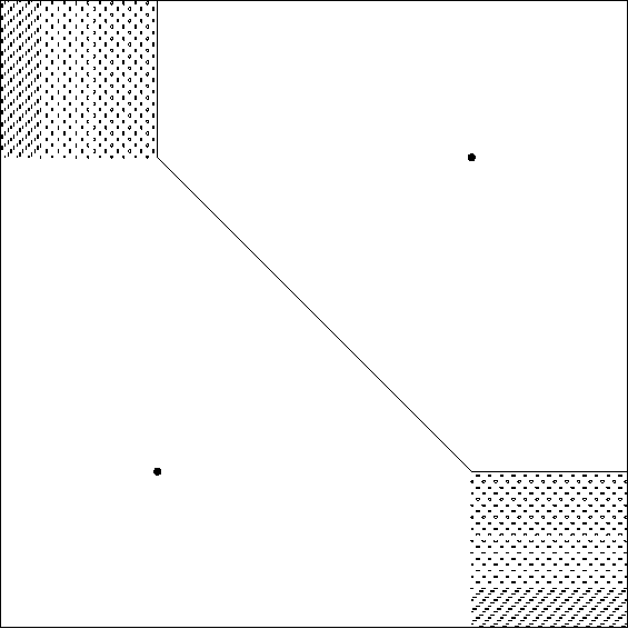 Figure 1
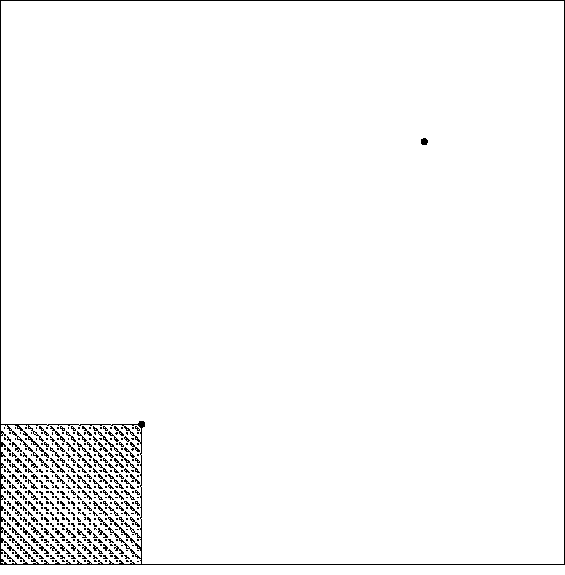 Figure 2
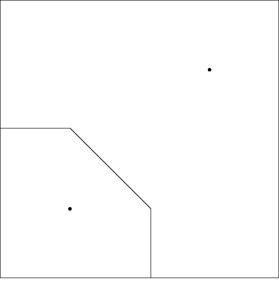 Figure 3
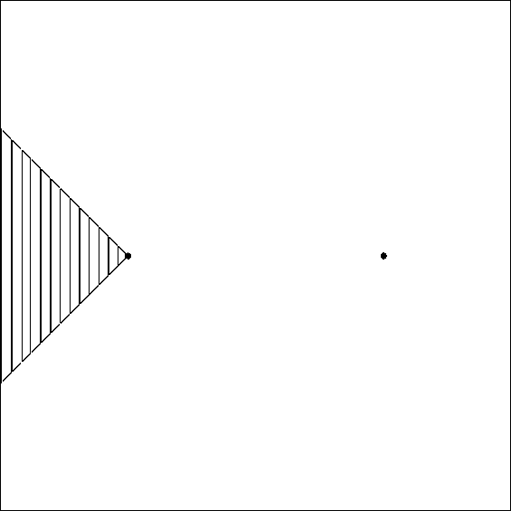 Figure 4
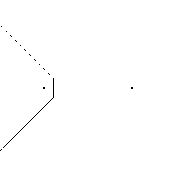 Figure 5
Peer Reviews
No public reviews on file for this paper yet. If you reviewed it on a platform where reviews are public (OpenReview, ICLR, NeurIPS, ICML), you can paste yours below so the community can read it here.
Videos
No videos yet. Explain this paper in a talk, walkthrough, or lecture? Add one.
Taxonomy
TopicsFacility Location and Emergency Management · Optimization and Variational Analysis
label=(), ref=(0)-()-()
Uniqueness of optimal solutions for semi-discrete transport with
-norm cost functions
J.D. Walsh III†
†School of Mathematics
Georgia Techn
Atlanta, GA 30332 U.S.A.
Tel.: +1 404-894-4401 Fax: +1 404-894-4409
Abstract.
Semi-discrete transport can be characterized in terms of real-valued shifts. Often, but not always, the solution to the shift-characterized problem partitions the continuous region. This paper gives examples of when partitioning fails, and offers a large class of semi-discrete transport problems where the shift-characterized solution is always a partition.
Key words and phrases:
Optimal transport and Monge-Kantorovich and semi-discrete and Wasserstein distance
1991 Mathematics Subject Classification:
65K10 and 90C08
Acknowledgments. This material is based upon work supported by the National Science Foundation Graduate Research Fellowship Program under Grant No. DGE-1650044. Any opinions, findings, and conclusions or recommendations expressed in this material are those of the authors and do not necessarily reflect the views of the National Science Foundation.
1. Introduction
Optimal transport offers a way to measure the distance between two probability spaces, and . In the class of transport problems known as semi-discrete optimal transport, the probability distribution on is almost-everywhere continuous and the probability distribution on is discrete, with points of positive measure. Given minimal assumptions, described below, the semi-discrete problem always has at least one solution that partitions into regions based on transport destination.
Rüschendorf and Uckelmann developed a way to characterize semi-discrete transport in terms of a set of real-valued shifts. This shift characterization often results in a solution that partitions into regions. Unfortunately, the shift characterization does not always partition . This important fact has not always been recognized or clearly expressed in the literature; see [5, 6, 7]. To remedy that ambiguity, this paper gives clear, specific examples where shift-characterized partitioning fails, and it offers a large class of problems where the shift characterization is guaranteed to partition .
2. Background
2.1. General optimal transport: the Monge-Kantorovich and Monge
problems
Though this paper focuses on the semi-discrete problem, it is worth describing it in terms of the more general, Monge-Kantorovich transport problem.
Definition 2.1** (Monge-Kantorovich problem).**
Let , let and be probability densities defined on and , and let be a continuous measurable ground cost function. Define the set of transport plans
[TABLE]
where is the set of probability measures on the product space, and define the primal cost function as
[TABLE]
The Monge-Kantorovich problem is to find the optimal primal cost
[TABLE]
and an associated optimal transport plan
[TABLE]
Under the conditions given, an optimal transport plan, , is guaranteed to exist. However, may not be unique, or even a.e.-unique. Furthermore, the existence of , an optimal plan, does not ensure that is a map, or that an optimal map exists. Nonetheless, consider the form such an optimal map would take.
Definition 2.2** (Monge problem).**
In certain cases, there exists at least one solution to the semi-discrete Monge-Kantorovich problem that does not split transported masses. In other words, there exists some such that
[TABLE]
where is a measurable map called the optimal transport map. When such a exists, we say the solution also solves the Monge problem.
If the Monge problem has a solution, we can assume without loss of generality that every satisfies
[TABLE]
for some measurable transport map , and that the primal cost can be written
[TABLE]
2.2. Semi-discrete optimal transport and the
shift characterization
The semi-discrete optimal transport problem is the Monge-Kantorovich problem of Definition 2.1, with restrictions on and :
- (1)
Assume that satisfies the following:
- (a)
is bounded. 2. (b)
is nonatomic. 3. (c)
is continuous except on a set of Lebesgue measure zero. 4. (d)
The support of is contained in the convex compact region . 2. (2)
Assume has exactly non-zero values, located at .
Because is continuous and is nonatomic, at least one solution to the semi-discrete Monge-Kantorovich problem also satisfies the Monge problem, described in Definition 2.2; see [4]. Thus, by applying Equation 2.6, we can assume without loss of generality that any transport plan has an associated map , and that partitions into sets , where is the set of points in that are transported by to . Using this partitioning scheme in combination with Equation 2.7 allows us to rewrite the primal cost function for the semi-discrete problem as
[TABLE]
This idea of sets is central to describing the shift characterization of the semi-discrete optimal transport problem. The following definition is based on one given by Rüschendorf and Uckelmann in [5, 7].
Definition 2.3** (Shift characterization).**
Let be a set of finite values, referred to as shifts. Define
[TABLE]
For , where , let
[TABLE]
Note that . The problem of determining an optimal transport plan is equivalent to determining shifts such that for all , the total mass transported from to equals .
2.3. Formalizing the shift-characterized partition
“Partitioning” is described in [7, 5] as . However, it is beneficial to describe the shift-characterized partition in more detail. Doing so requires a few additional definitions.
Definition 2.4** (Boundaries and boundary sets).**
For all such that , let
[TABLE]
The boundary set is defined as
[TABLE]
For all such that , define as
[TABLE]
Definition 2.5** ( -partitions ).**
Let be as defined in Equation 2.9, and the sets as defined in Equation 2.10 for . Then one says -partitions the set , or is called a -partition, if
- (1)
, 2. (2)
for all , , , 3. (3)
, and 4. (4)
for all , .
Definition 2.6** (Monge under the shift characterization).**
We say a transport plan is Monge under the shift characterization if has an associated transport map , a function , as described in Equation 2.9, and sets , as described in Equation 2.10, such that for all ,
[TABLE]
In other words, -partitions and agrees with on .
If for the shifts , no such transport plan can exist, and the transport problem itself can be said to be not Monge under the shift characterization. Conversely, if , then such a transport plan exists, and so the transport problem itself is said to be Monge under the shift characterization. In other words, -partitions if and only if the transport problem is Monge under the shift characterization.
The following result, from [3], allows us to go further:
Theorem 2.7**.**
Suppose one has a semi-discrete transport problem, as described in Section 2.2. Let be as defined in Equation 2.9, and the sets as defined in Equation 2.10 for . Then -partitions if and only if .
Taken together, these statements provide a formal definition and condition for what it means for the shift-characterized solution to partition :
The shift-characterized semi-discrete transport problem partitions — that is, -partitions — if and only if the semi-discrete transport problem is Monge under the shift characterization, which is true if and only if .
2.4. Uniqueness of semi-discrete transport
solutions
Given the semi-discrete transport problem described in Section 2.2, Corollary 4 of [2] provides a sufficient condition for the existence of a Monge solution that is unique -a.e.:
[TABLE]
If Equation 2.15 is satisfied, . Therefore, if Equation 2.15, then the transport problem is Monge under the shift characterization and the transport solution is unique -a.e.
However, if a transport problem is Monge under the shift characterization, then it has a unique -a.e. shift-characterized solution, whether or not Equation 2.15 is satisfied. This statement is formalized and proved in [3] as the following theorem:
Theorem 2.8** (The optimal transport map is unique -a.e.).**
Given a semi-discrete transport problem, let and be optimal transport plans that are both Monge under the shift characterization. If is a transport map associated with , and a transport map associated with , then except on a set of -measure zero.
3. Mathematical support
While Equation 2.15 implies , the converse is not true, as Section 3.1 shows. Next, Section 3.2 identifies a large class of problems where both conditions hold and the solution is always unique -a.e.
3.1. Partitioning with the 1-norm
and -norm
Let , , and let be the continuous uniform distribution. This simple setup can be used to demonstrate failure to partition for both the uniform norm (-norm) and the Manhattan norm (-norm).
3.1.1. The uniform norm
Let and , and let be the uniform norm (-norm): for all , . Consider two examples:
- (1)
If , then . In this case, , and the shift-characterized solution fails to partition . See Figure 1(a). 2. (2)
However, if , then , and the shift-characterized solution does partition . See Figure 1(b).
Even though one of the problems illustrated in Figure 1 results in a partition, Equation 2.15 fails in both cases:
[TABLE]
In general, for this choice of , , , and , the shift-characterized solution partitions if and only if
[TABLE]
Thus, when is the uniform norm, one can have , giving a shift-characterized partition of that is unique -a.e., whether or not Equation 2.15 is satsified.
3.1.2. The Manhattan norm
Now let and . Let be the Manhattan norm (1-norm): for all , . Consider three examples:
- (1)
If , then . In this case, , and the shift-characterized solution fails to partition . See Figure 2(a) for an illustration. 2. (2)
If , then and , so the shift-characterized solution again fails to partition . This is shown in Figure 2(b). 3. (3)
However, if , then . In this case and the shift-characterized solution does partition . See Figure 2(c).
Once again, Equation 2.15 fails in all the Figure 2 cases:
[TABLE]
In fact, for this choice of , , , and , the shift-characterized solution partitions if and only if
[TABLE]
Thus, as Figure 2 illustrates, when is the 1-norm, one can have , giving a shift-characterized partition of that is unique -a.e., whether or not Equation 2.15 is satsified.
Figure 2(a) is worth special consideration, because it is not simply a non-partitioning shift-characterized transport solution: it also constitutes a failed Voronoi diagram. One can see a similar example in Figure 37 of [1], offered as part of a discussion on methods for resolving lack of partitioning and uniqueness for certain Voronoi diagrams.
3.2. Partitioning with -norms when
-norm
Given the semi-discrete transport assumptions already stated, let be a -norm with :
[TABLE]
Then the semi-discrete transport problem is always Monge under the shift characterization.
This assertion will be shown in two steps:
- (1)
If , defined in Equation 2.13, is equal to the constant value in some neighborhood of , then . [Theorem 3.1] 2. (2)
It follows from Step (1) that implies the existence of a ball of positive radius whose points are all collinear with both and . [Theorem 3.2]
Because of the contradiction inherent in Step (2), , and so Theorem 3.2 concludes that the problem must be Monge under the shift characterization.
Theorem 3.1**.**
Let be a -norm with , and for some , . If for all in a neighborhood of , then .
Proof.
Let be a -norm with , , and for all in some neighborhood of . Suppose to the contrary, however, that .
Say , and assume without loss of generality that . Then
[TABLE]
which implies . This is a violation of the triangle inequality. Therefore, it must be the case that .
For all , define . Because , and . Hence, and .
Because is constant in a neighborhood of , , which implies . Hence, each of the first-order partial derivatives of and are equal at .
Assume , , and . Then the equality of the -th partial derivatives, , gives
[TABLE]
Thus, and have the same sign or are both zero. Because , . Hence, taking the -th root of both sides,
[TABLE]
As a consequence of Equation 3.2, if and only if . Hence, if and only if .
Let be the total number of -th directional components satisfying . Consider three cases: , , and .
**: **
Then for all , in which case . Since the semi-discrete transport problem requires distinct non-zero points in , it must be the case that , contradicting the initial assumption that . Hence, .
**: **
There exists exactly one such that the components are not equal. Since and have the same sign,
[TABLE]
This contradicts the assumption that , and hence .
**: **
Because is constant in some neighborhood of , it must also be the case that . Hence, , so each of the second-order partial derivatives of and are equal at . The equality of the second-order partial derivatives taken with respect to gives
[TABLE]
which can be rewritten as
[TABLE]
Applying Equation 3.2, define
[TABLE]
Then Equation 3.4 can be rewritten as
[TABLE]
By assumption, for all , and . Hence, .
Since , and for all , it must be that for all . Therefore,
[TABLE]
which implies . Therefore, , and Equation 3.5 simplifies to .
Thus, . Combining this with Equation 3.2 implies for all , and so . Since , and the semi-discrete transport problem requires distinct non-zero points in , it must be the case that , contradicting the initial assumption that . Thus, .
All choices of lead to contradictions. Hence, if is a -norm for some , , , and for all in some neighborhood of , then it must be the case that . ∎
Theorem 3.2**.**
If is a -norm for some , then the semi-discrete transport problem is Monge under the shift characterization.
Proof.
Assume the contrary is true. Then , so for some , . Because is nonatomic, there exist and such that the ball , defined with respect to the Euclidean space , satisfies and . By Theorem 3.1, . Assume without loss of generality that .
Let . Since ,
[TABLE]
Because is a -norm and , Minkowski’s inequality implies that , , and are all collinear. The choice of was nonspecific, and therefore every point in the ball must be collinear with the points and .
Of course, this is impossible, and so for all , . Therefore, . From this final contradiction, it is clear that the semi-discrete transport problem must be Monge under the shift characterization. ∎
Corollary 3.3**.**
If the semi-discrete transport problem is defined as given in Section 2.2, and is a -norm for some , then Equation 2.15 is satisfied, and the optimal transport solution is unique -a.e.
Proof.
Suppose is a -norm for some , and assume the semi-discrete transport problem is characterized by shifts as given in Definition 2.3. By the triangle inequality, for all , , , . Hence, one consequence of the triangle inequality is that for all , such that . Therefore, if or . This implies
[TABLE]
By Theorem 3.2, . Thus, for any , , . Since the problem assumes nothing about the probability density , it must be the case that
[TABLE]
Therefore, for all , , and for all , and uniqueness follows from Corollary 4 of [2]. ∎
4. Conclusions
This paper resolves issues of partitioning and uniqueness for semi-discrete transport problems using a large class of ground cost functions: the -norms. If the cost function is a -norm with , the above arguments ensure that -a.e. unique solutions exist for semi-discrete transport problems. As the examples show, if the cost function is a -norm with or , the solution may or may not constitute a -a.e. unique partition of the continuous space.
The reference list from the paper itself. Each links out to its DOI / PubMed record.
- 1[1] Franz Aurenhammer. Voronoi diagrams — A survey of fundamental geometric data structure. ACM Computing Surveys , 23(3):345–405, 1991.
- 2[2] Juan Antonio Cuesta-Albertos and Araceli Tuero-Díaz. A characterization for the solution of the Monge-Kantorovich mass transference problem. Statistics and Probability Letters , 16(2):147–152, 1993.
- 3[3] Luca Dieci and J.D. Walsh III. The boundary method for semi-discrete optimal transport partitions and Wasserstein distance computation. Preprint, ar Xiv:1702.03517 [math.NA], 2017.
- 4[4] Svetlozar Rachev and Ludger Rüschendorf. Mass Transportation Problems. Vol I: Theory, Vol II: Applications . Probability and its applications. Springer-Verlag, New York, 1998.
- 5[5] Ludger Rüschendorf. Monge-Kantorovich transportation problem and optimal couplings. Jahresbericht der Deutschen Mathematiker-Vereinigung , 109(3):113–137, 2007.
- 6[6] Ludger Rüschendorf and Ludger Uckelmann. On optimal multivariate couplings. In Distributions with given marginals and moment problems , pages 261–273. Kluwer Academic Publishers, 1997.
- 7[7] Ludger Rüschendorf and Ludger Uckelmann. Numerical and analytical results for the transportation problem of Monge-Kantorovich. Metrika , 51(3):245–258, 2000.