Numerical investigation of Differential Biological Models via RBF collocation Method with Genetic Strategy
Fardin Salehi, Soleiman Hashemi-Shahraki, Mohammad Kazem Fallah,, Mohammad Hemami

TL;DR
This paper combines the Kansa method with a genetic algorithm to optimize the shape parameter in RBF collocation for solving biological differential models, demonstrating improved accuracy and convergence.
Contribution
It introduces a genetic algorithm-based approach to select the optimal shape parameter in RBF collocation, enhancing solution accuracy for biological differential equations.
Findings
Genetic strategy effectively finds near-optimal shape parameters.
Pseudo-Combination crossover accelerates convergence.
Method improves solution accuracy for HIV and Influenza models.
Abstract
In this paper, we use Kansa method for solving the system of differential equations in the area of biology. One of the challenges in Kansa method is picking out an optimum value for Shape parameter in Radial Basis Function to achieve the best result of the method because there are not any available analytical approaches for obtaining optimum Shape parameter. For this reason, we design a genetic algorithm to detect a close optimum Shape parameter. The experimental results show that this strategy is efficient in the systems of differential models in biology such as HIV and Influenza. Furthermore, we prove that using Pseudo-Combination formula for crossover in genetic strategy leads to convergence in the nearly best selection of Shape parameter.
Click any figure to enlarge with its caption.
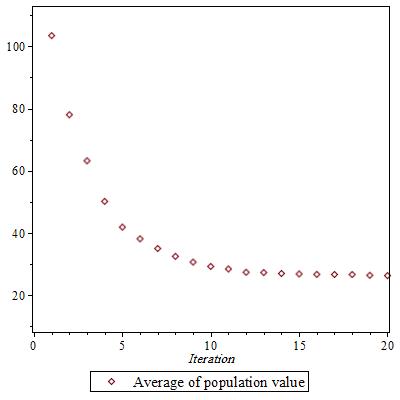 Figure 1
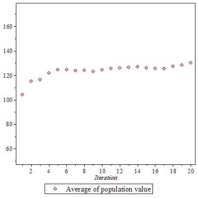 Figure 2
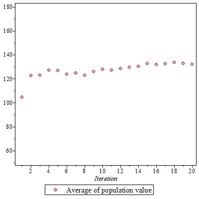 Figure 3
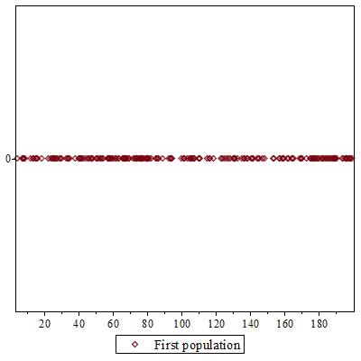 Figure 4
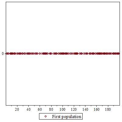 Figure 5
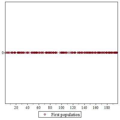 Figure 6
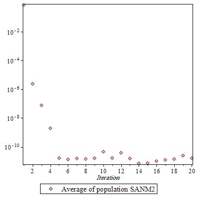 Figure 7
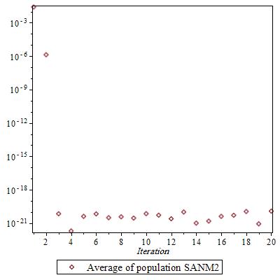 Figure 8
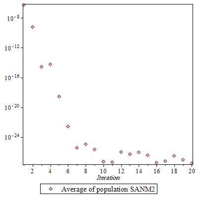 Figure 9
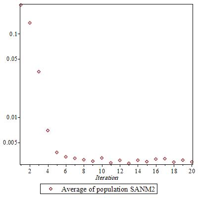 Figure 10
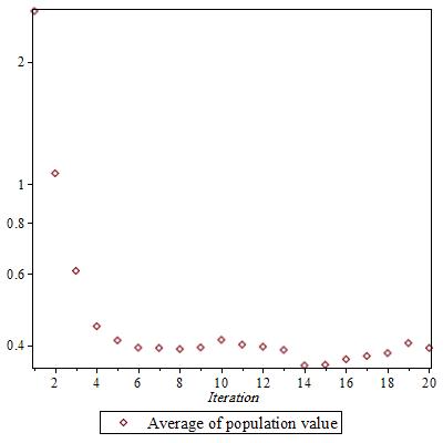 Figure 11
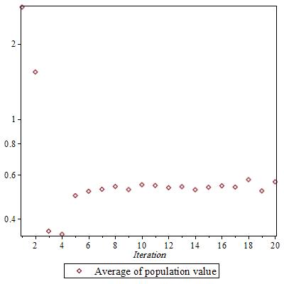 Figure 12
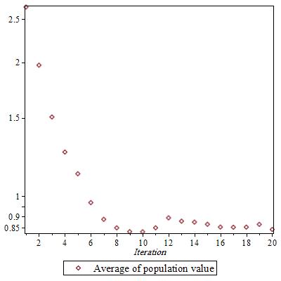 Figure 13
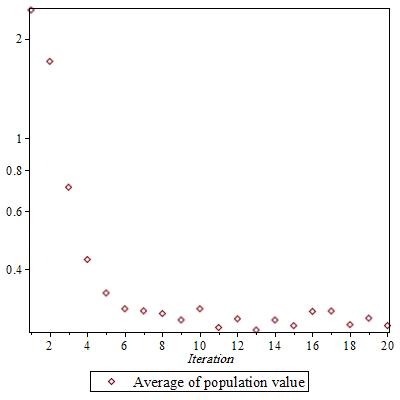 Figure 14
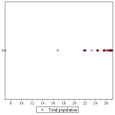 Figure 15
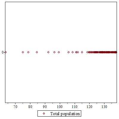 Figure 16
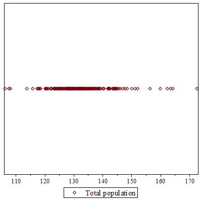 Figure 17
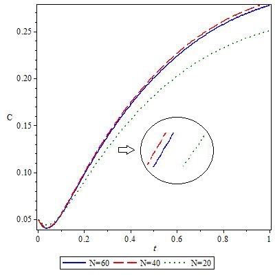 Figure 18
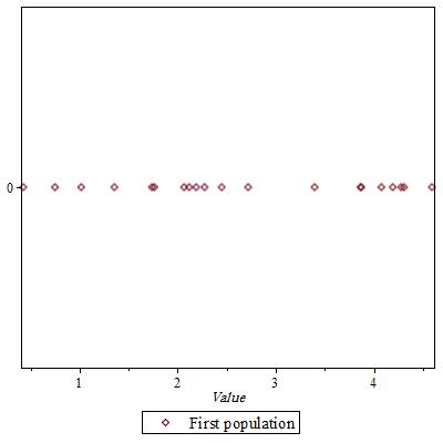 Figure 19
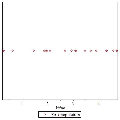 Figure 20
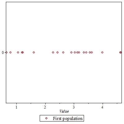 Figure 21
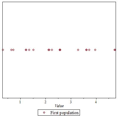 Figure 22
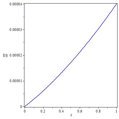 Figure 23
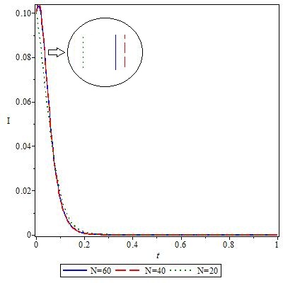 Figure 24
 Figure 25
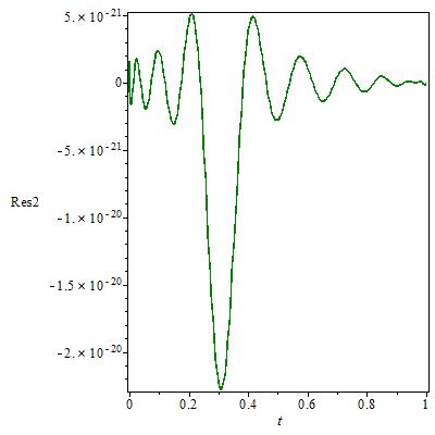 Figure 26
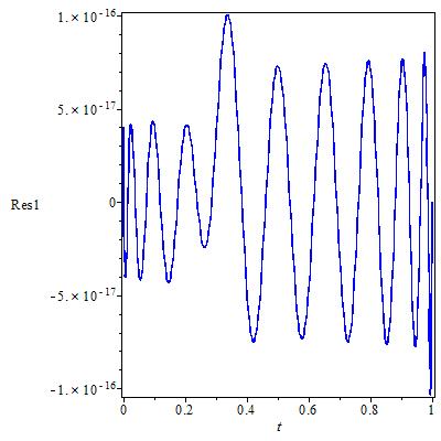 Figure 27
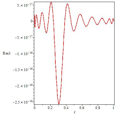 Figure 28
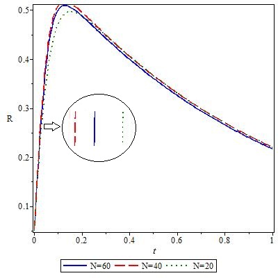 Figure 29
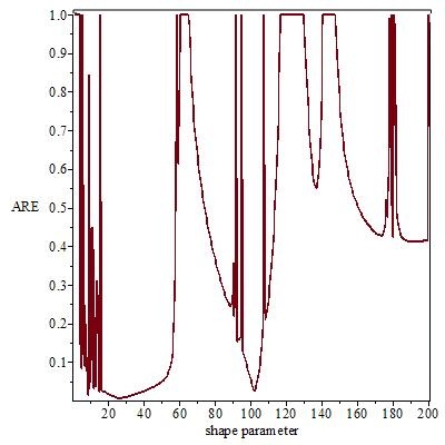 Figure 30
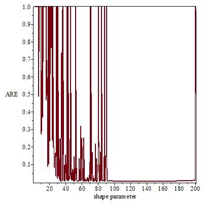 Figure 31
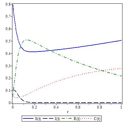 Figure 32
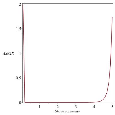 Figure 33
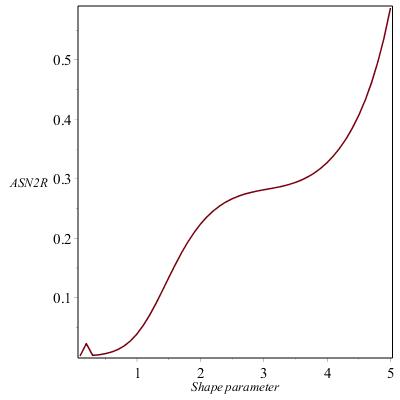 Figure 34
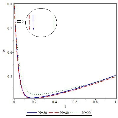 Figure 35
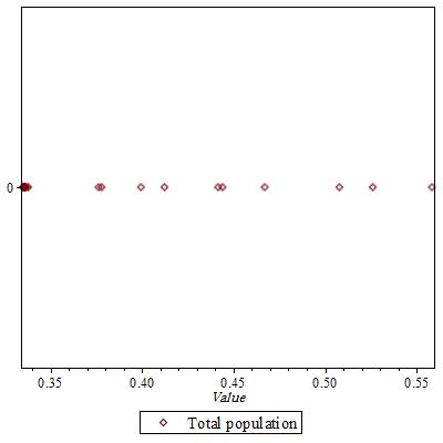 Figure 36
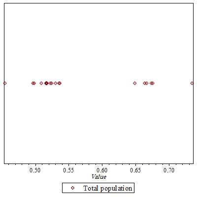 Figure 37
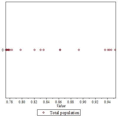 Figure 38
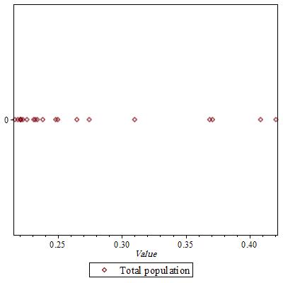 Figure 39
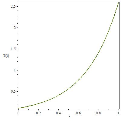 Figure 40
| Natural turnover rates of uninfected T cells | |
| Infected T cells | |
| Virus particles | |
| Infection rate | |
| Rate of constructing T cells | |
| Rate of T cells mitoses | |
| Virus particle from each infected T cell | |
| Maximum T cell concentration in the body |
| Author(s) | Method | Year |
|---|---|---|
| Merdan[44] | Homotopy Perturbation method(HPM) | 2007 |
| Alomari et al.[24] | Homotopy Analysis method(HAM) | 2011 |
| Merdan et al. [45] | Variational Iteration Method(VIM) | 2011 |
| Ongun[48] | Laplace Adomian Decomposition Method(LADM) | 2011 |
| Doğun[17] | Multistep Laplace Adomian Decomposition Method(MLADM) | 2012 |
| Khan et al.[40] | Iterative Homotopy Perturbation Transform Method(IHPTM) | 2012 |
| Yüzbaşi[73] | Bessel Collocation Method(BCM) | 2012 |
| Atangana et al.[5] | Homotopy Decomposition Method(HDM) | 2014 |
| Chen[11] | Padé-Adomian Decomposition Method(PADM) | 2015 |
| Venkatesh et al.[68] | Legendre Wavelets Method(LWM) | 2016 |
| Kajani et al.[23] | Müntz-Legendre Method(MLM) | 2016 |
| El-Baghdady et al.[18] | Legendre Collocation Method(LCM) | 2017 |
| Parand et al.[52] | Shifted Lagrangian Jacobi Method (SLG) | 2018 |
| Parand et al.[51] | Quasilinearization-Lagrangian Method (QLM) | 2018 |
| Parand et al.[53] | Pseudospectral Legendre Method (PLM) | 2018 |
| Parand et al.[52] | Shifted Boubaker Lagrangian Method (SBLM) | 2018 |
| Parand et al.[54] | Shifted Chebyshev Polynomial Method (SCP) | 2019 |
| Umar et al.[66] | Genetic Algorithm Active Set Method (GA-ASM) | 2020 |
| Oluwaseun et al.[47] | Block Method (BM) | 2021 |
| Thirumalai et al.[65] | Spectral Collocation Method (SCM) | 2021 |
| Umar et al.[67] | Neuro Swarm Intelligent Computing (NSIC) | 2021 |
| Hassani et al.[29] | Generalized Shifted Jacobi Polynomials (GSJP) | 2022 |
| Mortality rate | |
| Improve infection each year | |
| Progression from recovered to cross-immune each year | |
| Progression from recovered to susceptible each yer | |
| Rate of cross-immune into the infective | |
| Contact rate |
| Author(s) | Method | Year |
|---|---|---|
| El-Shahed et al.[19] | Non-standard Finite Difference(NSFDM) | 2012 |
| Ibrahim et al. [33] | Modified differential transform method(MDTM) | 2013 |
| Zeb et al.[74] | Multi-step generalized differential transform method(MGDTM) | 2013 |
| Khader et al.[38] | Chebyshev spectral method(CSM) | 2014 |
| Khader et al.[37] | Legendre spectral method(LSM) | 2014 |
| González-parra et al.[27] | Grünwald –Letnikov method(GLM) | 2014 |
| Class | Name of function | Definition |
|---|---|---|
| 1 | Multiquadrics(MQ) | |
| Inverse Multiquadrics (IMQ) | ||
| Gaussian (GA) | ||
| Inverse Quadrics (IQ) | ||
| Hyperbolic Secant (sech) | ||
| 2 | Thin Plate Spline (TPS) | |
| Conical Spline | ||
| 3 | Wendland3,0 | |
| Wu3,3 | ||
| Oscillator1,3 | ||
| Buhman1 | ||
| 4 | Plattea,b,c |
| t | BCM | RKM | HDM | LWM | Present method for N=20 |
|---|---|---|---|---|---|
| 0.2 | 0.2038616561 | 0.2088080833 | 0.2088072731 | 0.2088073215 | 0.2088080843 |
| 0.4 | 0.3803309335 | 0.4062405393 | 0.4061052625 | 0.4061245634 | 0.4062405427 |
| 0.6 | 0.6954623767 | 0.7644238890 | 0.7611467713 | 0.7641476415 | 0.7644238985 |
| 0.8 | 1.2759624442 | 1.4140468310 | 1.3773198590 | 1.3977746217 | 1.4140468518 |
| 1.0 | 2.3832277428 | 2.5915948020 | 2.3291697610 | 2.5571462314 | 2.5915948516 |
| t | BCM | Runge-Kutta | HDM | LWM | Present method for N=20 |
|---|---|---|---|---|---|
| 0.2 | 0.6247872e-5 | 0.6032702e-5 | 6.0327072e-5 | 0.6032704e-5 | 0.6032702e-5 |
| 0.4 | 0.1293552e-4 | 0.1315834e-4 | 1.3159161e-4 | 0.1316784e-4 | 0.1315834e-4 |
| 0.6 | 0.2035267e-4 | 0.2122378e-4 | 2.1268368e-4 | 0.2112628e-4 | 0.2122378e-4 |
| 0.8 | 0.2837302e-4 | 0.3017741e-4 | 3.0069186e-4 | 0.2998139e-4 | 0.3017742e-4 |
| 1.0 | 0.3690842e-4 | 0.4003781e-4 | 3.9873654e-4 | 0.3287654e-4 | 0.4003781e-4 |
| t | BCM | Runge-Kutta | HDM | LWM | Present method for N=20 |
|---|---|---|---|---|---|
| 0.2 | 0.0618799185 | 0.0618798433 | 0.0618799602 | 0.0618799076 | 0.0618798432 |
| 0.4 | 0.0382949349 | 0.0382948878 | 0.0383132488 | 0.0383234157 | 0.0382948877 |
| 0.6 | 0.0237043186 | 0.0237045501 | 0.0243917434 | 0.0238109873 | 0.0237045500 |
| 0.8 | 0.0146795698 | 0.0146803637 | 0.0099672189 | 0.0162138976 | 0.0146803636 |
| 1.0 | 0.0237043186 | 0.0091008450 | 0.0033050764 | 0.0160504423 | 0.0091008449 |
| t | N=5 | Res | N=10 | Res | N=15 | Res | N=20 | Res |
|---|---|---|---|---|---|---|---|---|
| c=0.21635819 | c=0.33489998 | T(t) | c=0.51637831 | c=0.77428513 | ||||
| 0.2 | 0.2141496490 | 3.86e-03 | 0.2088094672 | 7.82e-06 | 0.2088080843 | 2.60e-13 | 0.2088080843 | 3.96e-17 |
| 0.4 | 0.3996040883 | 1.31e-01 | 0.4062432618 | 7.24e-07 | 0.4062405427 | 1.68e-13 | 0.4062405427 | 4.87e-17 |
| 0.6 | 0.7116524148 | 1.34e-01 | 0.7644289795 | 4.05e-07 | 0.7644238985 | 1.55e-13 | 0.7644238985 | 4.65e-17 |
| 0.8 | 1.2973641582 | 4.31e-03 | 1.4140559835 | 6.47e-07 | 1.4140468518 | 3.61e-13 | 1.4140468518 | 7.23e-17 |
| 1.0 | 2.3892259227 | 5.66e-92 | 2.5916114131 | 1.94e-84 | 2.5915948516 | 3.17e-80 | 2.5915948516 | 8.88e-78 |
| I(t) | ||||||||
| 0.2 | 0.6114687e-5 | 2.27e-09 | 0.6032719e-5 | 2.46e-11 | 0.6032702e-5 | 3.42e-18 | 0.6032702e-5 | 4.46e-21 |
| 0.4 | 0.1337344e-4 | 8.34e-07 | 0.1315841e-4 | 5.26e-14 | 0.1315834e-4 | 6.28e-18 | 0.1315834e-4 | 3.71e-21 |
| 0.6 | 0.2134401e-4 | 1.13e-06 | 0.2122391e-4 | 6.30e-13 | 0.2122378e-4 | 5.06e-18 | 0.2122378e-4 | 1.09e-21 |
| 0.8 | 0.2987347e-4 | 3.22e-08 | 0.3017760e-4 | 1.60e-12 | 0.3017742e-4 | 7.01e-19 | 0.3017742e-4 | 6.41e-22 |
| 1.0 | 0.3908961e-4 | 6.10e-96 | 0.4003806-4 | 4.41e-89 | 0.4003781e-4 | 9.99e-85 | 0.4003781e-4 | 1.45e-81 |
| V(t) | ||||||||
| 0.2 | 0.0618187051 | 6.80e-05 | 0.0618798524 | 6.92e-08 | 0.0618798432 | 4.57e-14 | 0.0618798432 | 5.14e-17 |
| 0.4 | 0.0384572762 | 2.28e-03 | 0.0382948935 | 6.31e-09 | 0.0382948877 | 7.37e-14 | 0.0382948877 | 4.08e-17 |
| 0.6 | 0.0242145096 | 2.31e-03 | 0.0237045544 | 3.49e-09 | 0.0237045500 | 7.32e-14 | 0.0237045500 | 1.22e-17 |
| 0.8 | 0.0151695545 | 7.31e-05 | 0.0146803662 | 5.55e-09 | 0.0146803636 | 4.63e-14 | 0.0146803636 | 1.00e-17 |
| 1.0 | 0.0093128300 | 3.10e-93 | 0.0091008467 | 2.11e-86 | 0.0091008449 | 6.50e-82 | 0.0091008449 | 4.10e-79 |
| RKFM | Presented method 20N | Presented method 40N | Presented method 60N | Relative error 60N | |
| S(t) | |||||
| c | - | 26.800747761 | 137.9078869 | 123.44438040 | - |
| 0.2 | 0.4129967652 | 0.4270195495 | 0.4098921081 | 0.4128015008 | 1.952644e-04 |
| 0.4 | 0.4280199934 | 0.4363880004 | 0.4246103505 | 0.4278128844 | 2.071090e-04 |
| 0.6 | 0.4502002535 | 0.4549500702 | 0.4463055244 | 0.4499962534 | 2.040001e-04 |
| 0.8 | 0.4765242244 | 0.4766921230 | 0.4719383037 | 0.4763283175 | 1.959069e-04 |
| 1.0 | 0.5054118548 | 0.5003541451 | 0.5001004305 | 0.5052268175 | 1.850373e-04 |
| I(t) | |||||
| c | - | 26.800747761 | 137.9078869 | 123.44438040 | - |
| 0.2 | 7.340828e-04 | 1.396989e-03 | 7.051238e-04 | 7.534934e-04 | 0.194106e-04 |
| 0.4 | 1.675623e-06 | 8.708980e-06 | 1.566126e-06 | 1.806640e-06 | 1.310170e-07 |
| 0.6 | 2.525609e-09 | 8.678259e-08 | 4.611322e-09 | -1.672634e-09 | 4.198243e-09 |
| 0.8 | 9.855557e-10 | -3.67796e-07 | -2.23659e-09 | -1.066306e-09 | 2.0518617e-09 |
| 1.0 | -7.72143e-10 | -2.21603e-05 | -1.428391e-09 | -3.324845e-08 | 3.2476307e-08 |
| R(t) | |||||
| c | - | 26.800747761 | 137.9078869 | 123.44438040 | - |
| 0.2 | 0.4886071026 | 0.4886065768 | 0.4957432281 | 0.4884197981 | 1.873045e-04 |
| 0.4 | 0.4001052933 | 0.4061157789 | 0.4061422515 | 0.3999667848 | 1.385085-e04 |
| 0.6 | 0.3262752258 | 0.3313413846 | 0.3312018206 | 0.3261621289 | 1.130969e-04 |
| 0.8 | 0.2660651578 | 0.2702079076 | 0.2700828333 | 0.2659730573 | 9.210050e-05 |
| 1.0 | 0.2169661278 | 0.2203903869 | 0.2202819063 | 0.2168965849 | 6.954290e-05 |
| C(t) | |||||
| c | - | 26.800747761 | 137.9078869 | 123.44438040 | - |
| 0.2 | 0.0976620493 | 0.9008003610 | 0.0990852949 | 0.0975773248 | 8.472450e-05 |
| 0.4 | 0.1718730376 | 0.1556924837 | 0.1741092475 | 0.1717627291 | 1.103085e-04 |
| 0.6 | 0.2235245180 | 0.2019667950 | 0.2263417601 | 0.2233978645 | 1.266535e-04 |
| 0.8 | 0.2574106166 | 0.2323192884 | 0.2606042265 | 0.2572747238 | 1.358928e-04 |
| 1.0 | 0.2776220180 | 0.2504052565 | 0.2810922415 | 0.2774868004 | 1.352176e-04 |
Peer Reviews
No public reviews on file for this paper yet. If you reviewed it on a platform where reviews are public (OpenReview, ICLR, NeurIPS, ICML), you can paste yours below so the community can read it here.
Videos
No videos yet. Explain this paper in a talk, walkthrough, or lecture? Add one.
Taxonomy
TopicsMathematical Biology Tumor Growth · Fractional Differential Equations Solutions
\corraddr
Mohammad Hemami
Numerical investigation of Differential Biological Models via RBF collocation Method with Genetic Strategy
Fardin Salehi 1a
Soleiman Hashemi-Shahraki 2a and Mohammad Kazem Fallah 3a and Mohammad Hemami 4a,b
a Department of Computer and Data Sciences, Faculty of Mathematical Sciences, Shahid Beheshti University, Tehran, Iran,
b Department of Cognitive Modeling, Institute for Cognitive and Brain Sciences, Shahid Beheshti University, Tehran, Iran.
Abstract
In this paper, we use radial basis function collocation method for solving the system of differential equations in the area of biology. One of the challenges in RBF method is picking out an optimal value for shape parameter in Radial basis function to achieve the best result of the method because there are not any available analytical approaches for obtaining optimal shape parameter. For this reason, we design a genetic algorithm to detect a close optimal shape parameter. The experimental results show that this strategy is efficient in the systems of differential models in biology such as HIV and Influenza. Furthermore, we show that using our pseudo-combination formula for crossover in genetic strategy leads to convergence in the nearly best selection of shape parameter.
keywords:
Radial basis function; Genetic algorithm; HIV; Influenza; Shape parameter
\MOS
65L05; 65L60
1 Introduction
In the past few years, various mathematical models have been used to investigate biological and clinical problems. Various examples of mathematical models have been presented hitherto, including HIV[56, 57], Influenza[36], Covid-19[69, 60] and Ebola[10, 3]. In this paper, we will focus specifically on the simulation of HIV and Influenza models using the combination of RBF method and genetic algorithm and we show that this method is very efficient and robust for simulating biological models.
1.1 HIV Infection CD4+T Cells
Acquired Immune Deficiency Syndrome (AIDS), first-time appeared in the continent of America in 1981[9]. The human immunodeficiency Virus (HIV) in short HIV is the cause of the illness that attacks vital cells such as Dendrite cells, helper lymphocyte particularly CD4+T cells and infects them and gradually, the immune system will be destroyed[14]. This process may take from 6 months to 10 years. The mathematical model of HIV-infected CD4+T cells described by Perelson and Nelson in 1991[56, 57]. HIV model investigates the concentration of susceptible CD4+T cells infected by the HIV viruses. It is obvious that presenting a mathematical model is an easier study of the behavior of the system and helps the process of detecting or improving disease. Let be the concentration of susceptible CD4+T cells, be CD4+T cells infected by the HIV virus and be free HIV particular in the blood at the time. Thus, the mathematical model of the HIV-infected CD4+T cell on a couple system of the ordinary differential equation will be presented as follows:
[TABLE]
where is a positive constant and other parameters have been shown in Table 1.
It is noteworthy that there is no exact solution for HIV model. Ergo, the numerical methods are used to solve it. Table 2 shows some approaches applied to this model.
1.2 Influenza
Influenza virus causes a type of disease named Influenza or Flu that is divided into four classes A, B, C and D[43]. From the perspective of the epidemic, class A is the most significant class. That is because this type is able to merge and rebuild its genes with host gene[4, 70]. The mathematical model of Susceptible-Infected-Removed (SIRC) for displaying the outbreaks of Influenza in population is defined by Kermack and McKendrick [36]. This is a system of the differential equation as follows:
[TABLE]
where and mean ratio susceptible, infections, recovered and cross immune respectively. Other parameters are shown in Table 3.
This model studied by Khader et al.[38] using Chebyshev spectral method in 2014. Table 4 shows the applying methods to SIRC model.
1.3 Meshfree Method
Firstly, the Meshfree methods introduced by Monaghan and Gingold in 1977. They enlarged a Lagrangian method according to Kernel estimate method[25]. A number of meshfree methods such as smoothing particle hydrodynamic (SPH)[63, 12], Element-Free Galerkin (EFG)[41, 8], Reproducing Kernel method (RKM)[1, 7], Meshless local Petrov-Galerkin (MLPG)[58, 6], Comapctly supported radial basis function method(CSRBF)[31, 39], Radial basis function finite difference method(RBFFD)[46, 30], Radial basis function differential quadrature method(RBF-DQ)[50, 49] and Kansa method (KM)[55, 62] are used for solving differential equations (DEs). The appearance of meshfree methods was through the difficulty of the classic methods such as Finite Element method (FEM)[64, 34] and Finite Difference method (FDM)[16, 15] which require a mesh of points for solving problems. In these methods, rising problem dimensions causes increasing complexity (the order of construction of the mesh); furthermore, in meshfree we have no need to make any grid, and scattered points are used instead. RBF method as a meshfree approach utilizes as Trial functions of kind (Global/Compact support) Radial basis functions (RBFs)Table 5 demonstrates the RBF types. The main advantages of RBF method are the simplicity, high accuracy, and capability of being applicable in high dimension problems. In addition to these advantages, there exist two main challenges that all methods based on RBFs are faced with; selecting Shape parameters (SP) and distribution of collocation points. Choosing an inappropriate SP decreases the performance of method or even it will be unusable when the method is ill-conditioned. It seems that amount of optimal Shape parameter (oSP) depends on equation state, dimension and etc. Thus, any comprehensive formula not found hitherto for recognizing optimal SP in RBFs. Instead of choosing a proper SP, Many researchers offered different formulas; however, these formulas are applicable only in some special cases. In [42] SP decomposed to a dimensionless size of support domain and a nodal spacing near the point at the center , where . Hardy [28] suggested using (inverse) multiquadric formula as follows:
[TABLE]
where , and is the distance of the center from its closest neighbor. Rippa[59] used the Predictive residual sum of square (PRESS) algorithm for calculating a proper SP. Leave on-out cross validation (LOOCV) approach [22]and Craven and Wahba [13] which emanated in the statistics literature used for finding optimal SP. Esmaeilbeigi et al. [2, 20] employed the genetic package of MATLAB for solving a number of DEs. The following formula is proposed in [35, 61] to calculate a reasonable SP
[TABLE]
where is the number of points and is the smallest and is the biggest selected parameter in the domain of candidate SPs. Similarly, in [61, 72] the SP is obtained by
[TABLE]
where is a random number in arbitrary domain.
In this paper, we suggested a Meta-heuristic continues Genetic algorithm (CGA) choose a near optimal SP, based on the average of summation of the residual 2-norm (ASN2R) and the average of summation of the relative error (ARE) for the solution of differential equation systems in Biology sciences.
1.4 Genetic Algorithm
Genetic algorithm (GA) is a search and optimization approach based on the Genetic principles and natural selection. A GA starts with processing a population of candidate solutions (called individuals or chromosomes) with different competencies. During this process (called evolution), GA changes the population and generates some solutions close to optimal competency (maximum benefit or minimum cost). John Holland invented original GA in the early 1970s[32]. He also proposed a theoretical basis for GA according to the Type theory. In the following, David E Goldberg[26] extended GA concept and applied it to encode and solve different problems in miscellaneous fields. GA has many advantages over other optimization methods like:
- •
Practicable on both discrete and continuous data,
- •
No need to derivative of objective function (fitness function),
- •
Usable in multivariate functions,
- •
High potential for parallelization,
- •
Calculating a set of appropriate (close to optimal) solutions,
- •
Expandable on experimental, analytical and numerical data.
The main objective of a meta-heuristic algorithm is finding a close-minimum to global minimum (maximum) solution by escaping from local minimum (maximum) solutions. Universally, GA is classified to DGA (Discrete GA) and CGA (Continuous GA). In this article, we use CGA to find a close to optimal SP (-optimal Shape parameter) around a specified interval in the RBF method, where is either ASRN2 or ARE strategies.
2 Methodology
2.1 RBF approximation
Let be a continuous function with . A radial basis function on is a function of the form
[TABLE]
where , and denote the Euclidean distance between and s. By choosing points in and by defining
[TABLE]
where is called a radial basis functions mesh[71, 21]. To approximate one-dimensional function , we can illustrate it with an RBF as
[TABLE]
in which,
[TABLE]
is the input and s are the collection of coefficients to be determined. By selecting points () in interval:
[TABLE]
To sum up the discussion of the coefficients matrix, we define
[TABLE]
where
[TABLE]
By solving the system(4), the unknown coefficients will be attained.
2.2 Solving models by RBF method
Both models are system of first-order differential equations, so we define the solution functions and it’s first-order derivatives as follows:
[TABLE]
where is RBF. In addition, solution function and unknown coefficient are also defined separately according to the unknown functions of the models as follows
[TABLE]
for HIV and
[TABLE]
for Influenza model. Similarly, we define it’s derivative according to the Eq.(7). By placing the solution functions in the 1 and 2 equations, we form the residual functions for each system of equations as follows.
[TABLE]
for HIV and
[TABLE]
for Influenza.
We will simulate the problem in the domain (0, 1], and for this purpose we will choose the points within the domain, where we have used equidistant points. By placing the points in the residual functions and adding the initial conditions (IC#) as follows
[TABLE]
We obtain algebraic nonlinear equations for HIV model , as well as algebraic nonlinear equations for Influenza model as follows
[TABLE]
and finally for obtaining unknown coefficients, we solve these algebraic equations by Newton-Raphson method.
2.3 Genetic algorithm to find optimal shape parameter
GA as a meta-heuristic approach employed for optimization and finding the optimal parameter in problems. In fact, solving a problem by GA includes designing some functions and subroutines which be fired in each iteration (evolution). The main required functions and subroutines are Fitness function, Selection, Crossover, and mutation. However, more detailed explanation of GA is as follows:
Generating an initial population (chromosomes): The algorithm utilizes a population-based structure to solve the problem. Thus it is necessary to pick out an initial population from the solution domain and start the evolution. Generating the initial population is usually done by a uniformly random distribution. The commands ”sample(’Uniform’(, ),#points)” from the library ”Statistics” of Maple and ”rand(#points)” in Matlab generate the mentioned population. 2. 2.
Fitness function: In fitness function, the competency of each chromosome is investigated. The fitness of each individual is typically a numerical value. According to the nature of the problem, we assume that the minimum cost is zero and define our fitness function as:
[TABLE]
where is ASN2R () in HIV problem and ARE () in SIRC model. 3. 3.
Parental selection: GA is an iterative process, with the population in each iteration called a generation. The more fit individuals (parents) are stochastically selected from the current population, and modified (recombined and possibly randomly mutated) to form a new generation (children). Then the new generation of candidate solutions are used in the next iteration of the algorithm. Our method for selecting parents is based on the fitness function and Roulette wheel technique (RWT). In RWT, the chance of an individual to be chosen as a parent has a direct relationship with its fitness value. 4. 4.
Crossover: When two individuals are selected as parents, the crossover subroutines combine them to produce a new individual (their child). In this regard, we define a crossover formula called ”Pseudo-combination” (PCF). The PCF produces a child based on the value and fitness of its both parents. We define PCF as follows:
[TABLE]
where and parameters are child, first parent, second parent, outer limit and strongly inclination, respectively. The convergence of this PCF can be shown by taking the limit under different conditions as follows
- (a)
If and so
[TABLE]
because so
[TABLE] 2. (b)
If and so
[TABLE] 3. (c)
If and so
[TABLE]
because so
[TABLE] 4. (d)
If and so
[TABLE] 5. (e)
If so
[TABLE] 5. 5.
mutation: In mutation operation, some chromosomes are chosen randomly (according to the mutation rate) and one digit of each chromosome is replaced with a random digit. Considering elitism, we guard top three chromosomes (based on their fitness) against mutation.
Algorithm (1) presents a general form of the proposed GA.
3 Result
In this section, we set =0.02, = 0.016 =0.2 and =3, and solve the HIV(1) and Influenza SIRC(2) models. We used Maple 2015 for solving these models. The hardware configuration was as follows:
OS : Windows 10 (64bit)
CPU : Corei7 2.8 GHZ
RAM : 12 GB DDR3.
3.1 HIV
In HIV model, we approximate target functions with the classic Gaussian function and apply the average of residual functions to the fitness function. Figures 1 and 2 show given target function and residual function plots from 20 collocation points for T(t), I(t) and V(t).
Tables 6,7 and 8 illustrates the comparison of the presented method (with 20 collocation points) with approximated results of Bessel Collocation method (BCM)[73], Runge-Kutta method (RKM)[73], Homotopy Decomposition method (HDM)[5] and Wavelet Legendre method (WLM)[68]. The results show that the presented method and Runge-Kutta method are equal up to eight decimal places.
Figures 3 and 4 show the residual functions. We used the uniform distribution library of Maple and generate 20 chromosomes as GA initial population in search domain (0.1 , 5). The GA population collected on the smaller range after 20 iterations:
5 collocation points (0.1 , 5)(0.15 , 0.45)
10 collocation points (0.1 , 5) (0.3 , 0.59)
15 collocation points (0.1 , 5)(0.45 , 0.75)
20 collocation points (0.1 , 5)(0.74 , 0.95).
Figure 5 shows the condition of ASN2R based on the SP in the domain (0.1, 5). The optimal SP for 5 collocation points is in the domain (0.12, 0.35) and for 15 collocation points is in the domain (0.2, 0.8).
Obviously, by increasing the number of iterations in GA, in the case of the uniqueness of the optimal point, the final range will be limited again. Table 9 represents changes in the results and residuals by changing the number of collocation points. It can be seen that the results remained stable in 15 and 20 points.
In Fig. (6) and Fig. (7) display the average of value population (AVP) and the average of the residual population (ARP). After a number of steps, the AVP tended to a nonzero value, likewise, the ARP disposed to zero which indicates the convergence and productivity of our Genetic strategy.
3.2 Influenza
In this model, we applied the Gaussian function with a minor change as follows
[TABLE]
Moreover, the GA population is 200 randomly selected points from the real domain (1, 200). We used Maple’s DSOLVE tool for calculating the fitness of chromosomes and compared our results with Runge-Kutta-Fehlberg (RKF) method. Four target functions have been obtained from 60 collocation points whose plots are shown in Fig.(8). In addition, in Fig. (9), treatment of functions for 20, 40 and 60 collocation points are considered. Initial and total population are presented in Fig. (10) and Fig. (11).
When we set the number of collocation points to 20, 40 and 60, the final generation collected in ranges (22, 28), (100, 140) and (120, 150) respectively. Furthermore, convergence of APN to a nonzero value is searchable in Fig.(13). Figure 12 shows the condition of ARE based on the SP selected from the domain (1, 200). For 20 collocation points, the optimal SP is in the domain (20, 30) and for 40 collocation points is in the domain (100, 160).
Eventually, Tab.(10) displays the comparison of the proposed method (for 20, 40 and 60 collocation points) with RKF method. It shows that our results converge to the RKF method by increasing the number of collocation points.
4 Conclusion
In this study we have proposed an approximation technique to solve biological equations.The method is based on the collocation method and Gaussian radial basis function. We used a Genetic strategy to overcome the challenge of searching optimal Shape parameters in RBF method. Additionally we tested ASN2R for HIV and ARE for SIRC model in fitness function and a new crossover formula called Pseudo-combination defined for using the considered GA. Finally, we showed that our approach is applicable and accurate for the solving system of the differential equations such as HIV and Influenza models.
Acknowledgments
The authors are very grateful to anonymous referees for carefully reading this paper and their comments and suggestions, which have improved the quality of the paper
The reference list from the paper itself. Each links out to its DOI / PubMed record.
- 1[1] S. Abbasbandy, B. Azarnavid, and M. S. Alhuthali. A shooting reproducing kernel hilbert space method for multiple solutions of nonlinear boundary value problems. Journal of Computational and Applied Mathematics , 279:293–305, 2015.
- 2[2] F. Afiatdoust and M. Esmaeilbeigi. Optimal variable shape parameters using genetic algorithm for radial basis function approximation. Ain Shams Engineering Journal , 6(2):639–647, 2015.
- 3[3] F. Agusto. Mathematical model of ebola transmission dynamics with relapse and reinfection. Mathematical biosciences , 283:48–59, 2017.
- 4[4] R. M. Anderson and R. M. May. Infectious diseases of humans: dynamics and control . Oxford university press, 1992.
- 5[5] A. Atangana and E. F. Doungmo Goufo. Computational analysis of the model describing hiv infection of cd 4+ t cells. Bio Med research international , 2014, 2014.
- 6[6] S. N. Atluri and T. Zhu. A new meshless local petrov-galerkin (mlpg) approach in computational mechanics. Computational mechanics , 22(2):117–127, 1998.
- 7[7] B. Azarnavid, F. Parvaneh, and S. Abbasbandy. Picard-reproducing kernel hilbert space method for solving generalized singular nonlinear lane-emden type equations. Mathematical Modelling and Analysis , 20(6):754–767, 2015.
- 8[8] T. Belytschko, Y. Lu, L. Gu, and M. Tabbara. Element-free galerkin methods for static and dynamic fracture. International Journal of Solids and Structures , 32(17-18):2547–2570, 1995.