Implicit Regularization in Matrix Factorization
Suriya Gunasekar, Blake Woodworth, Srinadh Bhojanapalli, Behnam, Neyshabur, Nathan Srebro

TL;DR
This paper investigates how gradient descent on matrix factorizations implicitly promotes low-rank solutions, converging to the minimum nuclear norm solution under certain conditions.
Contribution
It provides empirical and theoretical evidence that small step sizes and initializations near zero lead gradient descent to the minimum nuclear norm solution in matrix factorization.
Findings
Gradient descent converges to minimum nuclear norm solution under specific conditions.
Small step sizes and initializations close to zero are crucial for implicit regularization.
Theoretical support for empirical observations on matrix factorization behavior.
Abstract
We study implicit regularization when optimizing an underdetermined quadratic objective over a matrix with gradient descent on a factorization of . We conjecture and provide empirical and theoretical evidence that with small enough step sizes and initialization close enough to the origin, gradient descent on a full dimensional factorization converges to the minimum nuclear norm solution.
Click any figure to enlarge with its caption.
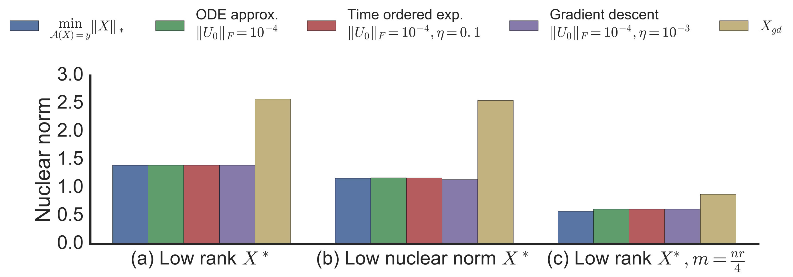 Figure 1
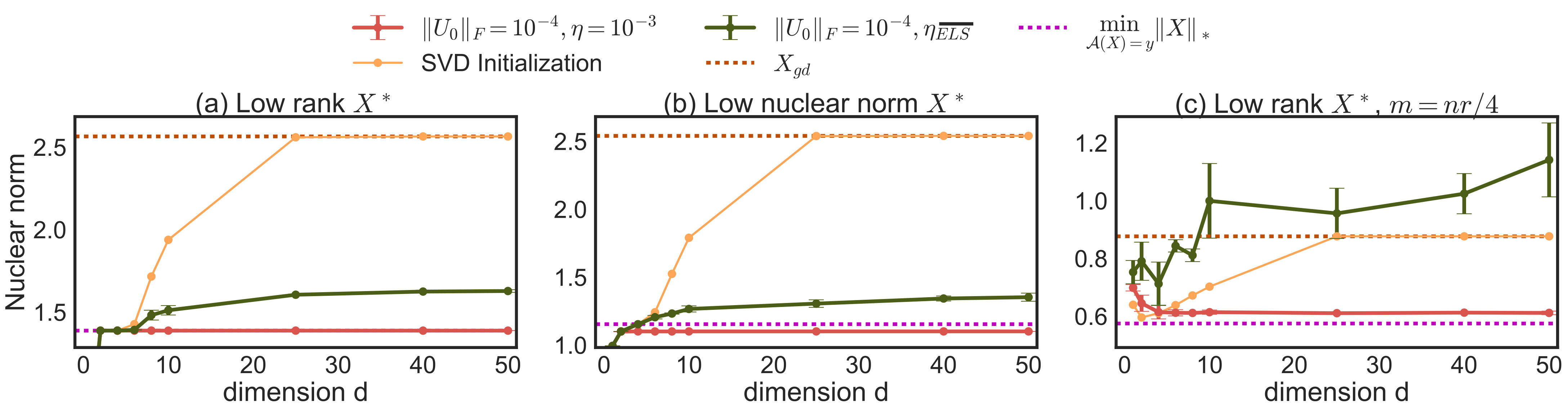 Figure 2
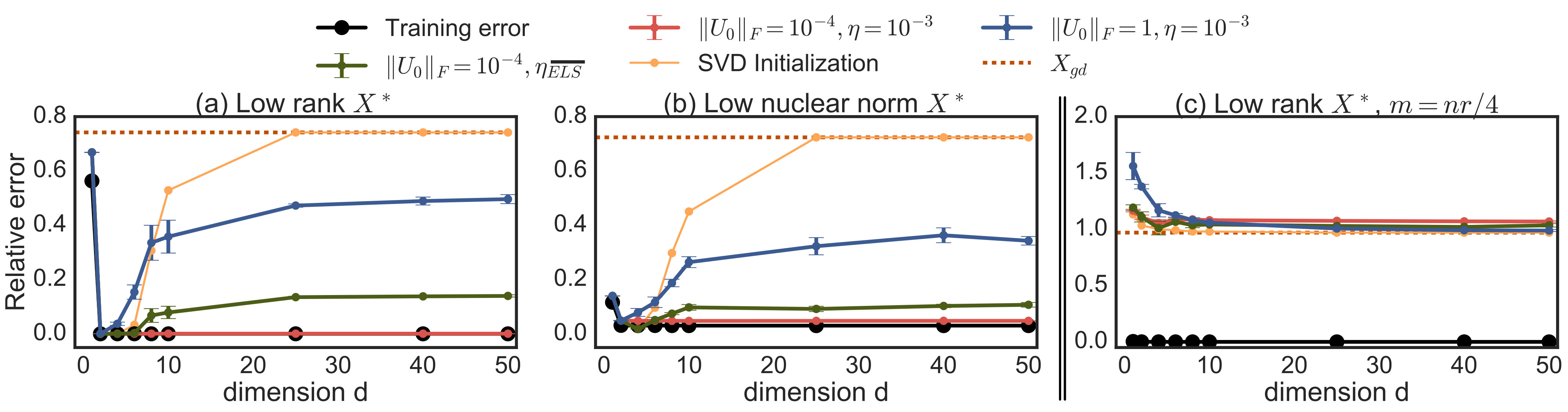 Figure 3
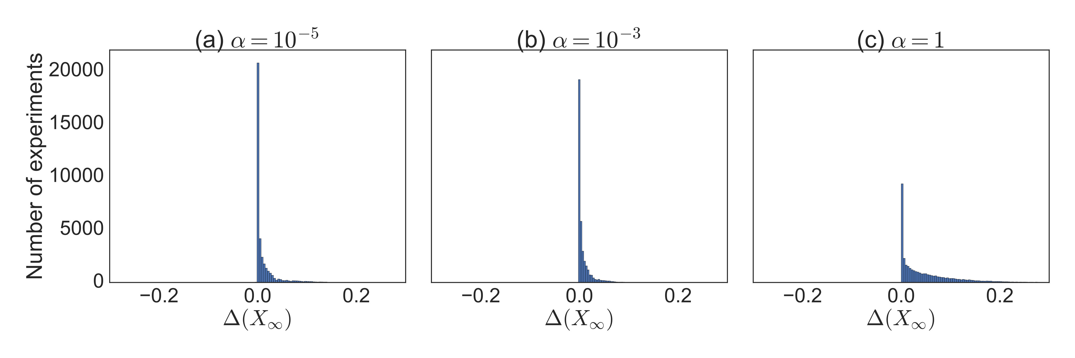 Figure 4
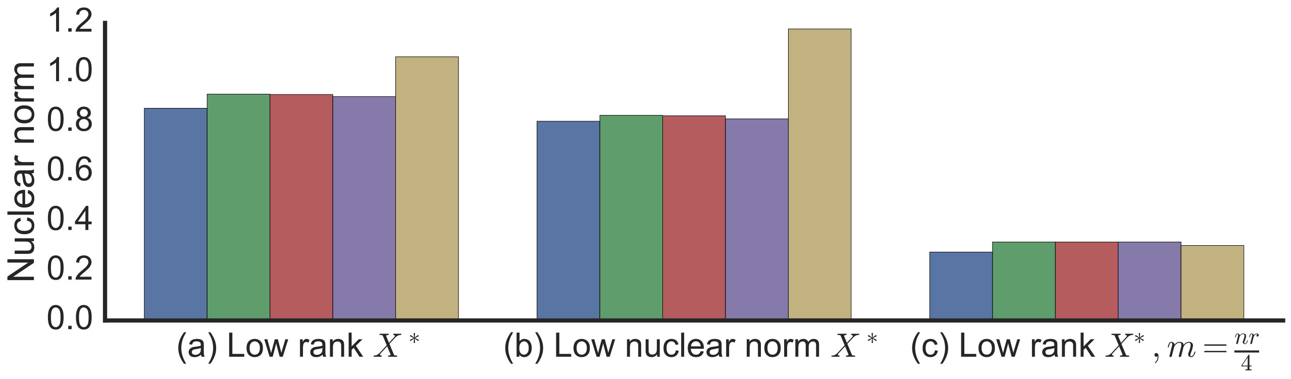 Figure 5
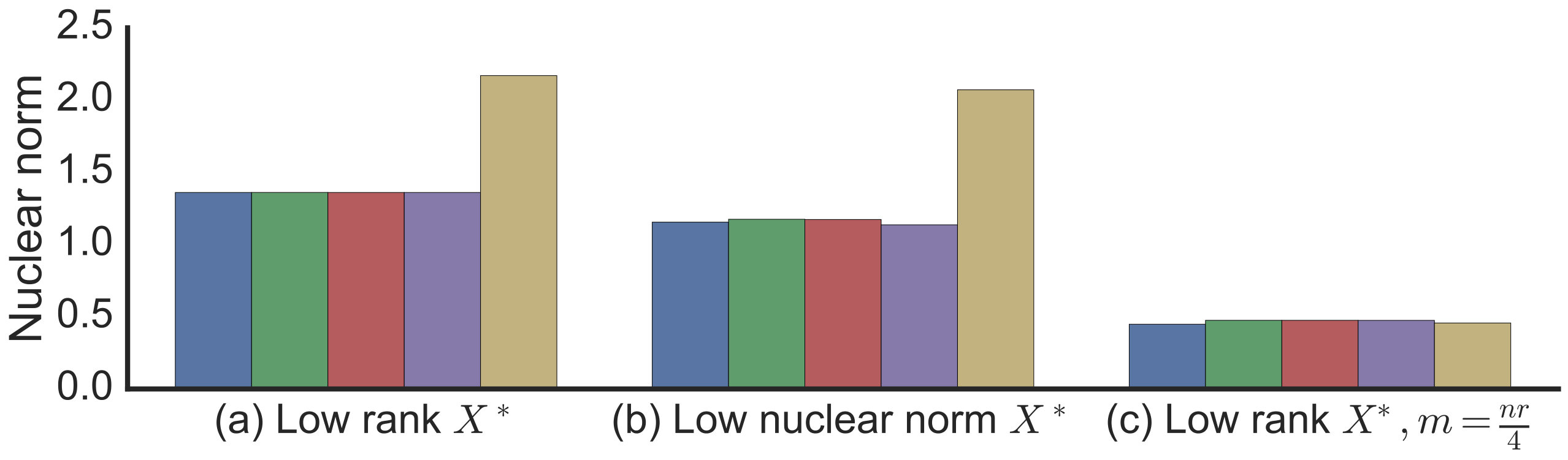 Figure 6
Peer Reviews
No public reviews on file for this paper yet. If you reviewed it on a platform where reviews are public (OpenReview, ICLR, NeurIPS, ICML), you can paste yours below so the community can read it here.
Videos
No videos yet. Explain this paper in a talk, walkthrough, or lecture? Add one.
Implicit Regularization in Matrix Factorization
\nameSuriya Gunasekar \[email protected] \AND\nameBlake Woodworth \[email protected] \AND\nameSrinadh Bhojanapalli \[email protected] \ANDBehnam Neyshabur \[email protected] \ANDNathan Srebro \[email protected]
Abstract
We study implicit regularization when optimizing an underdetermined quadratic objective over a matrix with gradient descent on a factorization of . We conjecture and provide empirical and theoretical evidence that with small enough step sizes and initialization close enough to the origin, gradient descent on a full dimensional factorization converges to the minimum nuclear norm solution.
1 Introduction
When optimizing underdetermined problems with multiple global minima, the choice of optimization algorithm can play a crucial role in biasing us toward a specific global minima, even though this bias is not explicitly specified in the objective or problem formulation. For example, using gradient descent to optimize an unregularized, underdetermined least squares problem would yield the minimum Euclidean norm solution, while using coordinate descent or preconditioned gradient descent might yield a different solution. Such implicit bias, which can also be viewed as a form of regularization, can play an important role in learning.
In particular, implicit regularization has been shown to play a crucial role in training deep models (Neyshabur et al., 2015, 2017; Zhang et al., 2017; Keskar et al., 2017): deep models often generalize well even when trained purely by minimizing the training error without any explicit regularization, and when there are more parameters than samples and the optimization problem is underdetermined. Consequently, there are many zero training error solutions, all global minima of the training objective, some of which my generalize horribly. Nevertheless, our choice of optimization algorithm, typically a variant of gradient descent, seems to prefer solutions that do generalize well. This generalization ability cannot be explained by the capacity of the explicitly specified model class (namely, the functions representable in the chosen architecture). Instead, it seems that the optimization algorithm biases us toward a “simple" model, minimizing some implicit “regularization measure”, and that generalization is linked to this measure. But what are the regularization measures that are implicitly minimized by different optimization procedures?
As a first step toward understanding implicit regularization in complex models, in this paper we carefully analyze implicit regularization in matrix factorization models, which can be viewed as two-layer networks with linear transfer. We consider gradient descent on the entries of the factor matrices, which is analogous to gradient descent on the weights of a multilayer network. We show how such an optimization approach can indeed yield good generalization properties even when the problem is underdetermined. We identify the implicit regularizer as the nuclear norm, and show that even when we use a full dimensional factorization, imposing no constraints on the factored matrix, optimization by gradient descent on the factorization biases us toward the minimum nuclear norm solution. Our empirical study leads us to conjecture that with small step sizes and initialization close to zero, gradient descent converges to the minimum nuclear norm solution, and we provide empirical and theoretical evidence for this conjecture, proving it in certain restricted settings.
2 Factorized Gradient Descent for Matrix Regression
We consider least squares objectives over matrices of the form:
[TABLE]
where is a linear operator specified by , , and . Without loss of generality, we consider only symmetric positive semidefinite (p.s.d.) and symmetric linearly independent (otherwise, consider optimization over a larger matrix with operating symmetrically on the off-diagonal blocks). In particular, this setting covers problems including matrix completion (where are indicators, Candès and Recht (2009)), matrix reconstruction from linear measurements (Recht et al., 2010) and multi-task training (where each column of is a predictor for a deferent task and have a single non-zero column, Argyriou et al. (2007); Amit et al. (2007)).
We are particularly interested in the regime where , in which case (1) is an underdetermined system with many global minima satisfying . For such underdetermined problems, merely minimizing (1) cannot ensure recovery (in matrix completion or recovery problems) or generalization (in prediction problems). For example, in a matrix completion problem (without diagonal observations), we can minimize (1) by setting all non-diagonal unobserved entries to zero, or to any other arbitrary value.
Instead of working on directly, we will study a factorization . We can write (1) equivalently as optimization over as,
[TABLE]
When , this imposes a constraint on the rank of , but we will be mostly interested in the case , under which no additional constraint is imposed on (beyond being p.s.d.) and (2) is equivalent to (1). Thus, if , then (2) with is similarly underdetermined and can be optimized in many ways — estimating a global optima cannot ensure generalization (e.g. imputing zeros in a matrix completion objective). Let us investigate what happens when we optimize (2) by gradient descent on .
To simulate such a matrix reconstruction problem, we generated random measurement matrices and set according to some planted . We minimized (2) by performing gradient descent on to convergence, and then measured the relative reconstruction error . Figure 1 shows the normalized training objective and reconstruction error as a function of the dimensionality of the factorization, for different initialization and step-size policies, and three different planted .
First, we see that (for sufficiently large ) gradient descent indeed finds a global optimum, as evidenced by the training error (the optimization objective) being zero. This is not surprising since with large enough this non-convex problem has no spurious local minima (Burer and Monteiro, 2003; Journée et al., 2010) and gradient descent converges almost surely to a global optima (Lee et al., 2016); there has also been recent work establishing conditions for global convergence for low (Bhojanapalli et al., 2016; Ge et al., 2016).
The more surprising observation is that in panels and , even when , indeed even for , we still get good reconstructions from the solution of gradient descent with initialization close to zero and small step size. In this regime, (2) is underdetermined and minimizing it does not ensure generalization. To emphasize this, we plot the reference behavior of a rank unconstrained global minimizer obtained via projected gradient descent for (1) on the space. For we also plot an example of an alternate “bad" rank global optima obtained with an initialization based on SVD of (‘SVD Initialization’).
When , we understand how the low-rank structure can guarantee generalization (Srebro et al., 2005) and reconstruction (Keshavan, 2012; Bhojanapalli et al., 2016; Ge et al., 2016). What ensures generalization when ? Is there a strong implicit regularization at play for the case of gradient descent on factor space and initialization close to zero?
Observing the nuclear norm of the resulting solutions plotted in Figure 2 suggests that gradient descent implicitly induces a low nuclear norm solution. This is the case even for when the factorization imposes no explicit constraints. Furthermore, we do not include any explicit regularization and optimization is run to convergence without any early stopping. In fact, we can see a clear bias toward low nuclear norm even in problems where reconstruction is not possible: in panel (c) of Figure 2 the number of samples is much smaller than those required to reconstruct a rank ground truth matrix . The optimization in (2) is highly underdetermined and there are many possible zero-error global minima, but gradient descent still prefers a lower nuclear norm solution. The emerging story is that gradient descent biases us to a low nuclear norm solution, and we already know how having low nuclear norm can ensure generalization (Srebro and Shraibman, 2005; Foygel and Srebro, 2011) and minimizing the nuclear norm ensures reconstruction (Recht et al., 2010; Candès and Recht, 2009).
Can we more explicitly characterize this bias? We see that we do not always converge precisely to the minimum nuclear norm solution. In particular, the choice of step size and initialization affects which solution gradient descent converges to. Nevertheless, as we formalize in Section 3, we argue that when is full dimensional, the step size becomes small enough, and the initialization approaches zero, gradient descent will converge precisely to a minimum nuclear norm solution, i.e. to .
3 Gradient Flow and Main Conjecture
The behavior of gradient descent with infinitesimally small step size is captured by the differential equation with an initial condition for . For the optimization in (2) this is
[TABLE]
where is the adjoint of and is given by . Gradient descent can be seen as a discretization of (3), and approaches (3) as the step size goes to zero.
The dynamics (3) define the behavior of the solution and using the chain rule we can verify that , where is a vector of the residual. That is, even though the dynamics are defined in terms of specific factorization , they are actually independent of the factorization and can be equivalently characterized as
[TABLE]
We can now define the limit point for the factorized gradient flow (4) initialized at . We emphasize that these dynamics are very different from the standard gradient flow dynamics of (1) on , corresponding to gradient descent on , which take the form .
Based on the preliminary experiments in Section 2 and a more comprehensive numerical study discussed in Section 5, we state our main conjecture as follows:
Conjecture**.**
For any full rank , if exists and is a global optima for (1) with , then .
Requiring a full-rank initial point demands a full dimensional factorization in (2). The assumption of global optimality in the conjecture is generally satisfied: for almost all initializations, gradient flow will converge to a local minimizer (Lee et al., 2016), and when any such local minimizer is also global minimum (Journée et al., 2010). Since we are primarily concerned with underdetermined problems, we expect the global optimum to achieve zero error, i.e. satisfy . We already know from these existing literature that gradient descent (or gradient flow) will generally converge to a solution satisfying ; the question we address here is which of those solutions will it converge to.
The conjecture implies the same behavior for asymmetric problems factorized as with gradient flow on , since this is equivalent to gradient flow on the p.s.d. factorization of .
4 Theoretical Analysis
We will prove our conjecture for the special case where the matrices commute, and discuss the more challenging non-commutative case. But first, let us begin by reviewing the behavior of straight-forward gradient descent on for the convex problem in (1).
Warm up:
Consider gradient descent updates on the original problem (1) in space, ignoring the p.s.d. constraint. The gradient direction is always spanned by the matrices . Initializing at , we will therefore always remain in the -dimensional subspace . Now consider the optimization problem . The KKT optimality conditions for this problem are and s.t. . As long as we are in , the second condition is satisfied, and if we converge to a zero-error global minimum, then the first condition is also satisfied. Since gradient descent stays on this manifold, this establishes that if gradient descent converges to a zero-error solution, it is the minimum Frobenius norm solution.
Getting started:
Consider the simplest case of the factorized problem when with and . The dynamics of (4) are given by , where is simply a scalar, and the solution for is given by, where . Assuming exists and , we want to show is an optimum for the following problem
[TABLE]
The KKT optimality conditions for (5) are:
[TABLE]
We already know that the first condition holds, and the p.s.d. condition is guaranteed by the factorization of . The remaining complementary slackness and dual feasibility conditions effectively require that is spanned by the top eigenvector(s) of . Informally, looking to the gradient flow path above, for any non-zero , as it is necessary that in order to converge to a global optima, thus eigenvectors corresponding to the top eigenvalues of will dominate the span of .
What we can prove: Commutative
The characterization of the the gradient flow path from the previous section can be extended to arbitrary in the case that the matrices commute, i.e. for all . Defining – a vector integral, we can verify by differentiating that solution of (4) is
[TABLE]
Theorem 1**.**
In the case where matrices commute, if exists and is a global optimum for (1) with , then .
Proof.
It suffices to show that such a satisfies the complementary slackness and dual feasibility KKT conditions in (6). Since the matrices commute and are symmetric, they are simultaneously diagonalizable by a basis , and so is for any . This implies that for any , given by (7) and its limit also have the same eigenbasis. Furthermore, since converges to , the scalars for each . Therefore, , where is defined as the eigenvalue corresponding to eigenvector and not necessarily the largest eigenvalue.
Let , then . For all such that , by the continuity of , we have
[TABLE]
Defining , we conclude that for all such that , . Similarly, for each such that ,
[TABLE]
Thus, for every , for sufficiently large
[TABLE]
Therefore, we have shown that and establishing the optimality of for (5). ∎
Interestingly, and similarly to gradient descent on , this proof does not exploit the particular form of the “control" and only relies on the fact that the gradient flow path stays within the manifold
[TABLE]
Since the ’s commute, we can verify that the tangent space of at a point is given by , thus gradient flow will always remain in . For any control such that following leads to a zero error global optimum, that optimum will be a minimum nuclear norm solution. This implies in particular that the conjecture extends to gradient flow on (2) even when the Euclidean norm is replaced by certain other norms, or when only a subset of measurements are used for each step (such as in stochastic gradient descent).
However, unlike gradient descent on , the manifold is not flat, and the tangent space at each point is different. Taking finite length steps, as in gradient descent, would cause us to “fall off" of the manifold. To avoid this, we must take infinitesimal steps, as in the gradient flow dynamics.
In the case that and the measurements are diagonal matrices, gradient descent on (2) is equivalent to a vector least squares problem, parametrized in terms of the square root of entries:
Corollary 2**.**
Let be the limit point of gradient flow on with initialization , where , and . If exists and , then .
The plot thickens: Non-commutative
Unfortunately, in the case that the matrices do not commute, analysis is much more difficult. For a matrix-valued function , is equal to only when and commute. Therefore, (7) is no longer a valid solution for (4). Discretizing the solution path, we can express the solution as the “time ordered exponential":
[TABLE]
where the order in the products is important. If commute, the product of exponentials is equal to an exponential of sums, which in the limit evaluates to the solution in (7). However, since in general , the path (12) is not contained in the manifold defined in (11).
It is tempting to try to construct a new manifold such that and , ensuring the gradient flow remains in . However, since ’s do not commute, by combining infinitesimal steps along different directions, it is possible to move (very slowly) in directions that are not of the form for any . The possible directions of movements indeed corresponds to the Lie algebra defined by the closure of under the commutator operator . Even when , this closure will generally encompass all of , allowing us to approach any p.s.d. matrix with some (wild) control . Thus, we cannot hope to ensure the KKT conditions for an arbitrary control as we did in the commutative case — it is necessary to exploit the structure of the residuals in some way.
Nevertheless, in order to make finite progress moving along a commutator direction like , it is necessary to use an extremely non-smooth control, e.g., looping times between steps in the directions , each such loop making an step in the desired direction. We expect the actual residuals to behave much more smoothly and that for smooth control the non-commutative terms in the expansion of the time ordered exponential (12) are asymptotically lower order then the direct term (as ). This is indeed confirmed numerically, both for the actual residual controls of the gradient flow path, and for other random controls.
5 Empirical Evidence
Beyond the matrix reconstruction experiments of Section 2, we also conducted experiments with similarly simulated matrix completion problems, including problems where entries are sampled from power-law distributions (thus not satisfying incoherence), as well as matrix completion problem on non-simulated Movielens data. In addition to gradient descent, we also looked more directly at the gradient flow ODE (3) and used a numerical ODE solver provided as part of SciPy (Jones et al., 2001). But we still uses a finite (non-zero) initialization. We also emulated staying on a valid “steering path" by numerically approximating the time ordered exponential of 12 — for a finite discretization , instead of moving linearly in the direction of the gradient (like in gradient descent), we multiply on right and left by . The results of these experiments are summarized in Figure 3.
In these experiments, we again observe trends similar to those in Section 2. In some panels in Figure 3, we do see a discernible gap between the minimum nuclear norm global optima and the nuclear norm of the gradient flow solution with . This discrepancy could either be due to starting at a non-limit point of , or numerical issue arising from approximations to the ODE, or it could potentially suggest a weakening of the conjecture. Even if the later case were true, the experiments so far provide strong evidence for atleast approximate versions of our conjecture being true under a wide range of problems.
Exhaustive search
Finally, we also did experiments on an exhaustive grid search over small problems, capturing essentially all possible problems of this size. We performed an exhaustive grid search for matrix completion problem instances in symmetric p.s.d. matrices. With , there are unique masks or ’s that are valid symmetric matrix completion observations. For each mask, we fill the observations with all possible combinations of uniformly spaced values in the interval . This gives us a total of problem instances. Of these problems instances, we discard the ones that do not have a valid PSD completion and run the ODE solver on every remaining instance with a random such that , for different values of . Results on the deviation from the minimum nuclear norm are reported in Figure 4. For small , most of instances of our grid search algorithm returned solutions with near minimal nuclear norms, and the maximum deviation is within the possibility of numerical error. This behavior also decays for .
6 Discussion
It is becoming increasingly apparent that biases introduced by optimization procedures, especially for under-determined problems, are playing a key role in learning. Yet, so far we have very little understanding of the implicit biases associated with different non-convex optimization methods. In this paper we carefully study such an implicit bias in a two-layer non-convex problem, identify it, and show how even though there is no difference in the model class (problems (1) and (2) are equivalent when , both with very high capacity), the non-convex modeling induces a potentially much more useful implicit bias.
We also discuss how the bias in the non-convex case is much more delicate then in convex gradient descent: since we are not restricted to a flat manifold, the bias introduced by optimization depends on the step sizes taken. Furthermore, for linear least square problems (i.e. methods based on the gradients w.r.t. in our formulation), any global optimization method that uses linear combination of gradients, including conjugate gradient descent, Nesterov acceleration and momentum methods, remains on the manifold spanned by the gradients, and so leads to the same minimum norm solution. This is not true if the manifold is curved, as using momentum or passed gradients will lead us to “shoot off” the manifold.
Much of the recent work on non-convex optimization, and matrix factorization in particular, has focused on global convergence: whether, and how quickly, we converge to a global minima. In contrast, we address the complimentary question of which global minima we converge to. There has also been much work on methods ensuring good matrix reconstruction or generalization based on structural and statistical properties. We do not assume any such properties, nor that reconstruction is possible or even that there is anything to reconstruct—for any problem of the form (1) we conjecture that (4) leads to the minimum nuclear norm solution. Whether such a minimum nuclear norm solution is good for reconstruction or learning is a separate issue already well addressed by the above literature.
We based our conjecture on extensive numerical simulations, with random, skewed, reconstructible, non-reconstructible, incoherent, non-incoherent, and and exhaustively enumerated problems, some of which is reported in Section 5. We believe our conjecture holds, perhaps with some additional technical conditions or corrections. We explain how the conjecture is related to control on manifolds and the time ordered exponential and discuss a possible approach for proving it.
The reference list from the paper itself. Each links out to its DOI / PubMed record.
- 1Amit et al. (2007) Yonatan Amit, Michael Fink, Nathan Srebro, and Shimon Ullman. Uncovering shared structures in multiclass classification. In Proceedings of the 24th international conference on Machine learning , pages 17–24. ACM, 2007.
- 2Argyriou et al. (2007) Andreas Argyriou, Theodoros Evgeniou, and Massimiliano Pontil. Multi-task feature learning. Advances in neural information processing systems , 19:41, 2007.
- 3Bhojanapalli et al. (2016) Srinadh Bhojanapalli, Behnam Neyshabur, and Nathan Srebro. Global optimality of local search for low rank matrix recovery. Advances in Neural Information Processing Systems , 2016.
- 4Burer and Monteiro (2003) Samuel Burer and Renato DC Monteiro. A nonlinear programming algorithm for solving semidefinite programs via low-rank factorization. Mathematical Programming , 95(2):329–357, 2003.
- 5Candès and Recht (2009) Emmanuel J Candès and Benjamin Recht. Exact matrix completion via convex optimization. Foundations of Computational mathematics , 9(6):717–772, 2009.
- 6Foygel and Srebro (2011) Rina Foygel and Nathan Srebro. Concentration-based guarantees for low-rank matrix reconstruction. In COLT , pages 315–340, 2011.
- 7Ge et al. (2016) Rong Ge, Jason D Lee, and Tengyu Ma. Matrix completion has no spurious local minimum. In Advances in Neural Information Processing Systems , pages 2973–2981, 2016.
- 8Jones et al. (2001) Eric Jones, Travis Oliphant, Pearu Peterson, et al. Sci Py: Open source scientific tools for Python, 2001. URL https://docs.scipy.org/doc/scipy-0.19.0/reference/generated/scipy.integrate.ode.html .