
TL;DR
This paper introduces a neural network-based method for generating pouring trajectories using force feedback, trained on demonstrations, and validated through simulation showing generalization to unseen pouring characteristics.
Contribution
It presents a novel force feedback-driven pouring trajectory generation approach utilizing recurrent neural networks trained on demonstration data.
Findings
System generalizes to unseen pouring characteristics
Force estimation system performs well in simulation
Neural network effectively predicts pouring velocity
Abstract
Pouring is a simple task people perform daily. It is the second most frequently executed motion in cooking scenarios, after pick-and-place. We present a pouring trajectory generation approach, which uses force feedback from the cup to determine the future velocity of pouring. The approach uses recurrent neural networks as its building blocks. We collected the pouring demonstrations which we used for training. To test our approach in simulation, we also created and trained a force estimation system. The simulated experiments show that the system is able to generalize to single unseen element of the pouring characteristics.
Click any figure to enlarge with its caption.
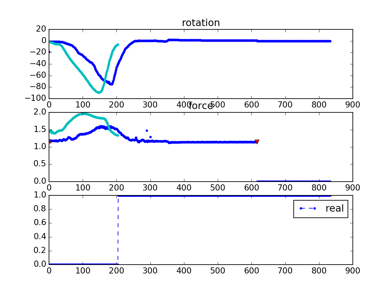 Figure 1
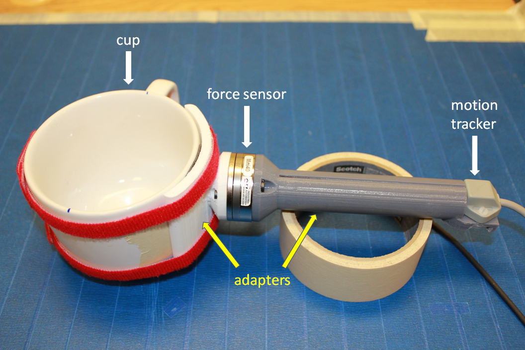 Figure 2
 Figure 3
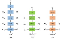 Figure 4
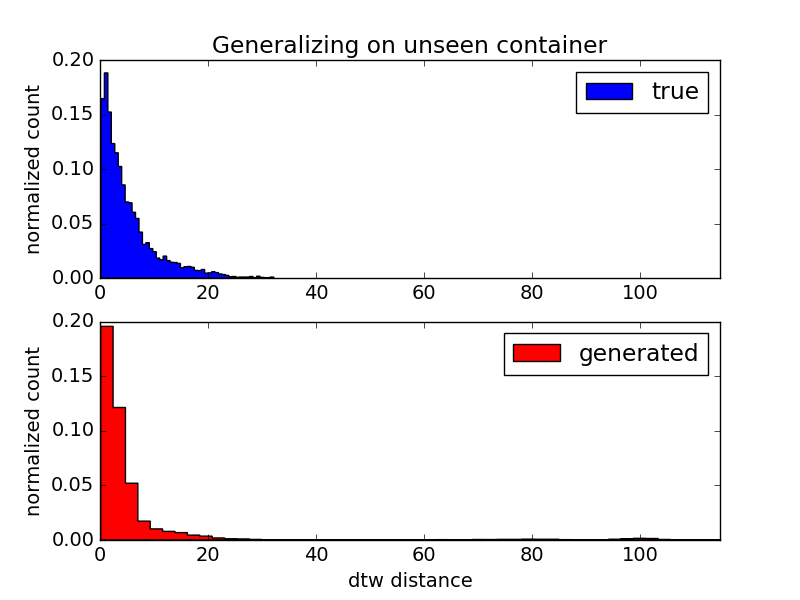 Figure 5
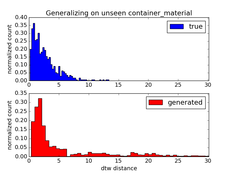 Figure 6
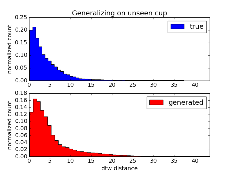 Figure 7
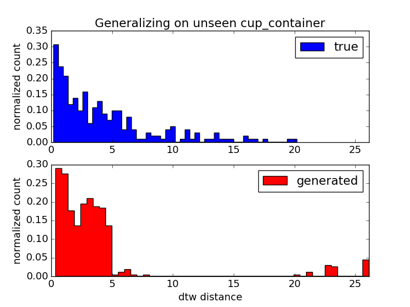 Figure 8
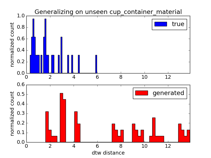 Figure 9
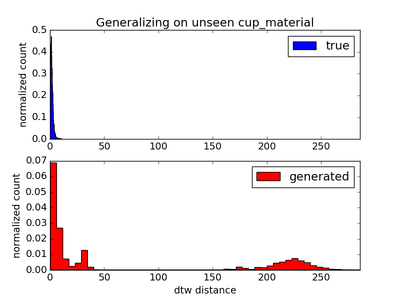 Figure 10
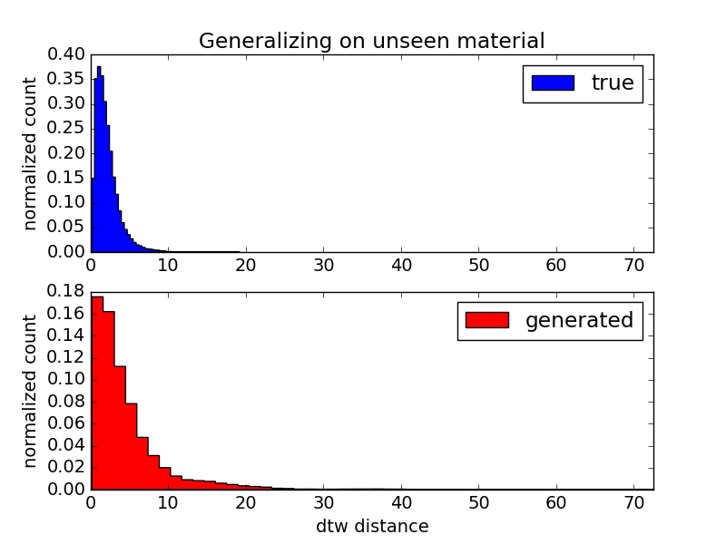 Figure 11
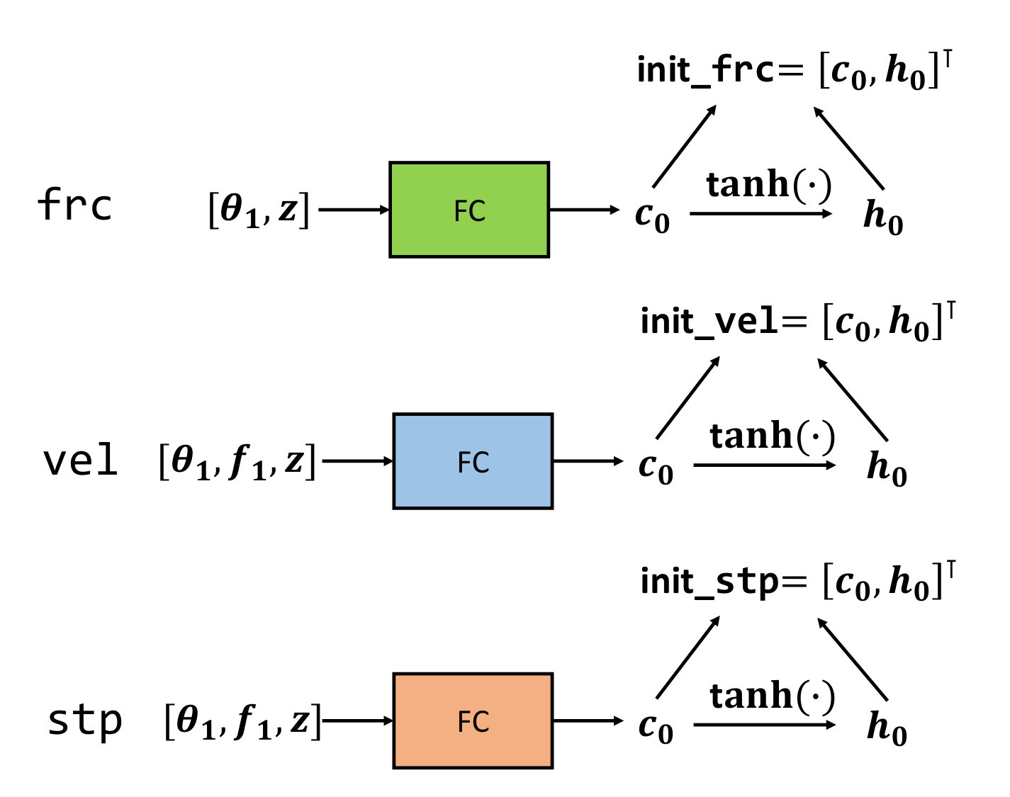 Figure 12
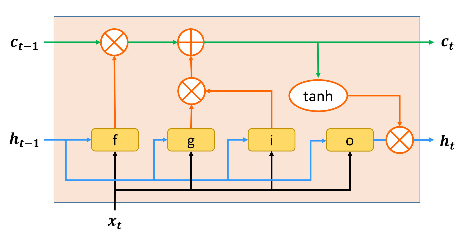 Figure 13
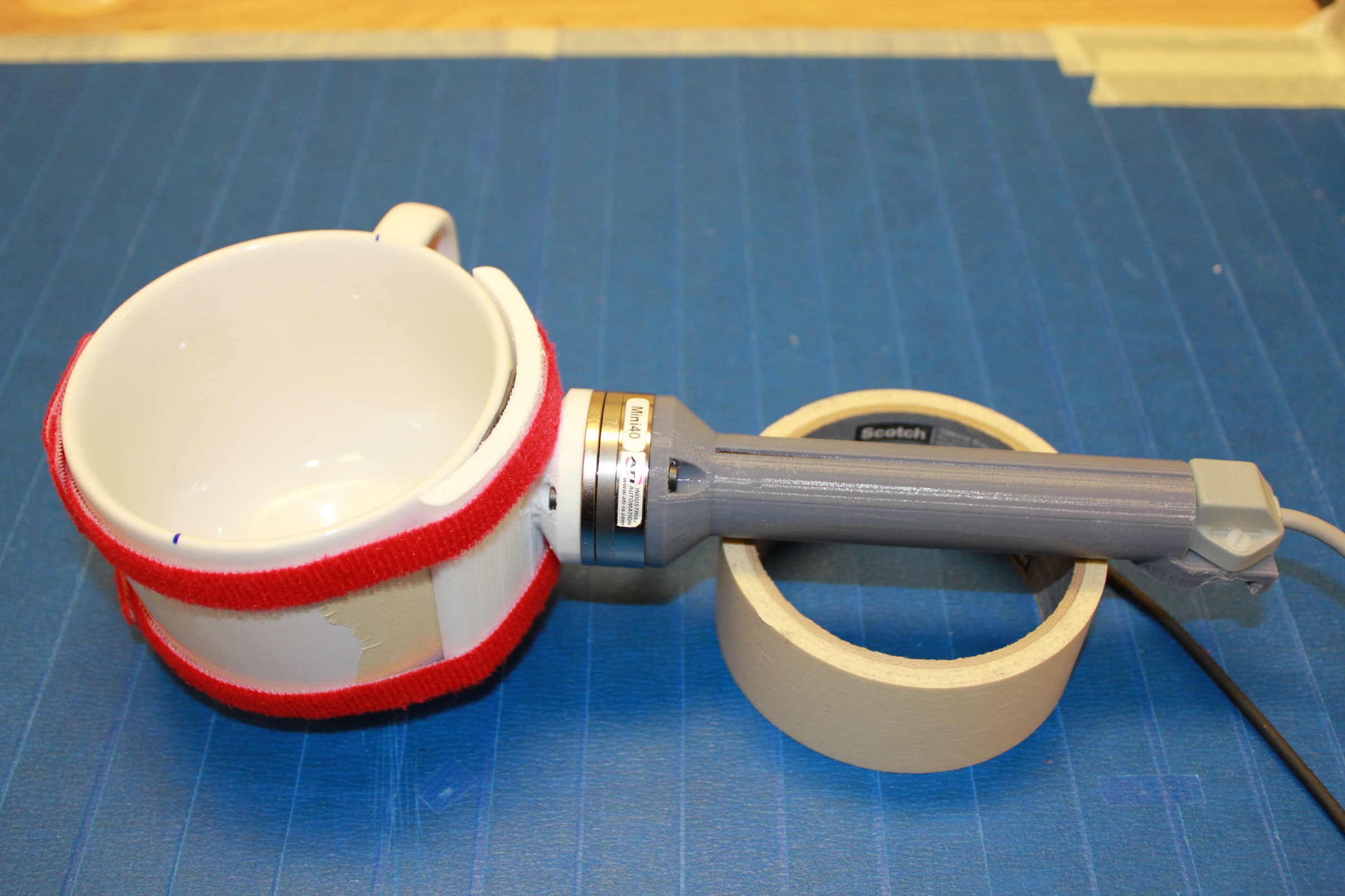 Figure 14
 Figure 15
 Figure 16
 Figure 17
 Figure 18
 Figure 19
 Figure 20
 Figure 21
 Figure 22
 Figure 23
 Figure 24
 Figure 25
 Figure 26
 Figure 27
 Figure 28
 Figure 29
 Figure 30
 Figure 31
 Figure 32
 Figure 33
 Figure 34
 Figure 35
 Figure 36
 Figure 37
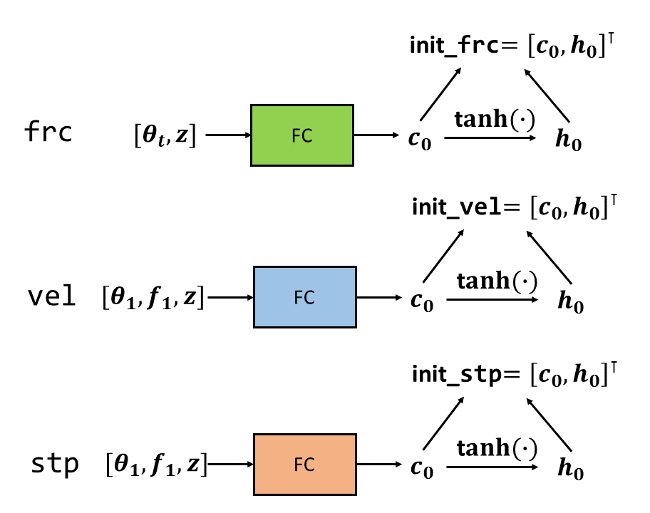 Figure 38
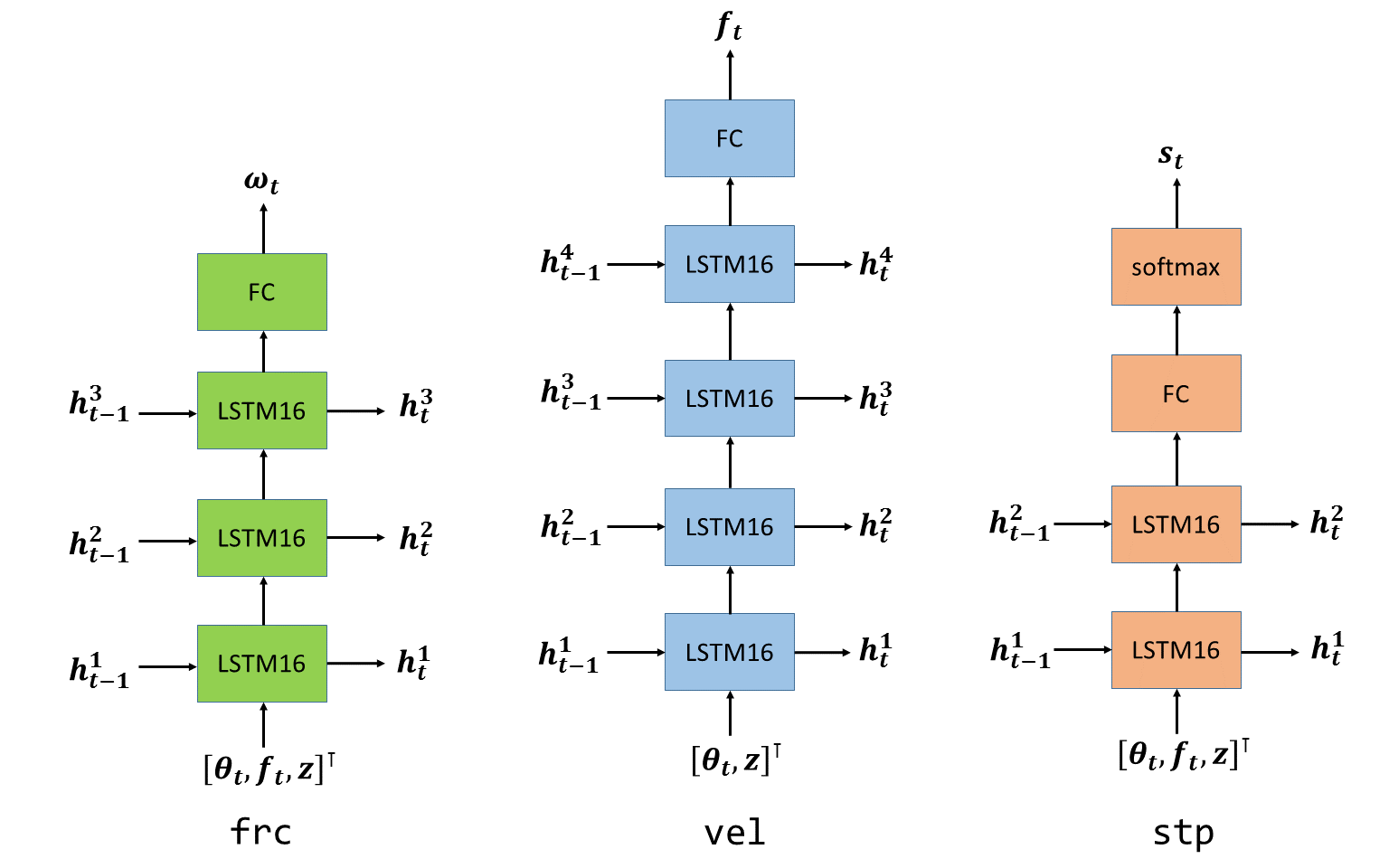 Figure 39
Peer Reviews
No public reviews on file for this paper yet. If you reviewed it on a platform where reviews are public (OpenReview, ICLR, NeurIPS, ICML), you can paste yours below so the community can read it here.
Videos
No videos yet. Explain this paper in a talk, walkthrough, or lecture? Add one.
Taxonomy
TopicsMusic and Audio Processing
Learning to Pour
Yongqiang Huang and Yu Sun The authors are with the Department of Computer Science and Engineering, University of South Florida, Tampa, FL 33620, USA. Email: [email protected], [email protected]
Abstract
Pouring is a simple task people perform daily. It is the second most frequently executed motion in cooking scenarios, after pick-and-place. We present a pouring trajectory generation approach, which uses force feedback from the cup to determine the future velocity of pouring. The approach uses recurrent neural networks as its building blocks. We collected the pouring demonstrations which we used for training. To test our approach in simulation, we also created and trained a force estimation system. The simulated experiments show that the system is able to generalize to single unseen element of the pouring characteristics.
I Introduction
Tasks that are found in manufacturing facilities are often precisely defined, repetitive, and tolerates very little error. Those tasks can be easily handled by industrial robots but proves difficult for human workers. In contrast, each time a daily activity is performed by human, its execution is adjusted according to the environment and is different from last time. Programming an industrial robot to accomplish the same is prohibitively difficult, whereas human completes those tasks with ease. To make robots more widely useful, researchers have been trying to help robots learn a task and generalize to different situations, to which the approach of teaching robots by providing examples has received considerable attention, known as programming by demonstration (PbD) [1]. In this work, we consider learning a task on the level of motion trajectories, and to perform a task, we generate a new trajectory.
Pouring is a simple task that human practice daily. It is the second most frequently executed motion in cooking scenarios after pick-and-place [2]. It relies on rotating a cup (or a container in general) that holds certain material. Sufficient rotation of the cup makes the material come out and sufficient recovery makes the pouring stop. Human typically pour using vision, while sensing the force resulted from the cup. We aim to learn from data how to pour using force feedback alone.
One popular framework for motion trajectory generation is dynamical movement primitives (DMP) [3]. DMP is a stable non-linear dynamical system, and is capable of modeling discrete movement such as swinging a tennis racket [4], playing table tennis [5] as well as rhythmic movement such as drumming [6] and walking [7]. DMP consists of a non-linear forcing function, a canonical system and a transformation system. The forcing function defines the desired task trajectory. The transformation system is a point attractor system for discrete movement or a limit cycle system for rhythmic movement that is modulated by the forcing function. The canonical system is a well-understood dynamical system that is guaranteed to converge and also serves to provide the phase variable of a task. The parameters that represent the forcing function can be learned from human demonstrations using locally weighted regression [8] or other regression methods.
Based on DMP, [9] introduced interactive primitives for two-agent collaborative tasks. A predictive distribution of the parameters of DMP is maintained and is used to infer the collaborative activity of one agent while observing that of the other. [10] extends [9] by using a Gaussian mixture of interactive primitives. Such extension allows the correlation between two agents of a collaboration task to be non-linear, and it also enables modeling multiple collaborative tasks.
Another approach for motion generation is based on Gaussian mixture model (GMM) and Gaussian mixture regression (GMR) [11]. GMM is used to model the trajectories of a task and GMR is used for task reproduction. GMM is learned using all the variables of a movement including time stamps, and GMR is conducted by infering the movement variables using the learned GMM conditioned on the time stamp. The parameters of GMM can be learned using the Expectation-Maximization algorithm [12]. Several constraints can be incorporated using the product property of Gaussians while performing a new task. The approach can be applied to both world and joint space to consider the trade-off of variations in difference spaces and thus achieves a more accurate control [13]. Also, task-parameterized GMM models a movement using multiple candidate frames of reference, and thus enables more detailed motion production [14]. Using time as the index the approach can produce a task trajectory in a single shot. In comparison, the approach can be extended to model a dynamical system which produces a trajectory step by step [15].
Principal Component Analysis (PCA) also proves useful for motion generation. Known as a dimension reduction technique used on the dimentionality axis of the data, PCA can be used on the time axis of motion trajectories instead to retrieve geometric variations [16]. Besides, PCA can also be applied to find variations in how the motion progresses in time, which, combined with the variations in geometry enables generating motions with more flexibility [17]. Functional PCA (fPCA) extends PCA by introducing continuous-time basis functions and treating trajectories as functions instead of collections of points [18]. [19] applies fPCA for producing trajectories of gross motion such as answering phone and punching, and for making the trajectories avoid obstacles with the guidance of quality via points. [2] uses fPCA for generating trajectories of fine motion such as pouring.
Recently, recurrent neural networks (RNN) receives increasing attention. At any time step, RNN takes a given input and the output emitted from the last time step, and emits an output which is passed to the next time step. The mechanism of RNN makes it inherently suitable for handling sequential data. Similar to DMP [3] and GMR based approach [15], RNN is also capable of modeling general dynamical systems [20, 21]. RNN can be readily used to generate trajectories by relating the emitted output to future inputs. For example, [22] generates English hand writing trajectories by predicting the location offset of the tip of the pen and the end of a stroke. [23] applies a similar strategy to generate Chinese characters. [24] generates motion capture trajectories by directly predicting the joint angle vector for the next time step.
The paper goes as follows. In Section II, we review the fundamentals of RNN and particularly LSTM, and present our pouring system. In Section III, we describe the data collection and preparation process, training the system, and creating and training a separate force estimation system. In Section IV, we conduct experiments to evaluate whether our system generalizes to unseen situations. We discuss the performance of our pouring system in Section V.
II Methodology for Pouring Trajectory Generation
In this section, we describe in detail our system of generating a pouring trajectory which builds on long short-term memory. To explain why we choose RNN as the building block, prior to the system description, we review the basics of traditional RNN, and of one particular structure, the long short-term memory.
II-A Recurrent Neural Network
Recurrent neural network (RNN) conducts its computation one step at a time, and at any step its input consists of two parts: a given input, and its own output from the previous time step. The idea is shown in Eq. (1) where is the given input, and are output from the previous and at the current step. The weight and bias can be learned using Backpropagation Through Time [25].
[TABLE]
In theory, by including its past output in its input, RNN takes the entire history of given inputs into account when it conducts computation at any step, and therefore is inherently suitable for handling sequential data. However, the traditional RNN as shown in Eq. (1) is difficult to train and has vanishing gradients problem, and therefore is inadequate for problems involving long-term dependency [26, 27]. Long short-term memory (LSTM) is a specific RNN design that overcomes the vanishing gradient problem [27]. We use a version of LSTM whose working mechanism is described by [28]:
[TABLE]
where are the input, output, and forget gates respectively, is the cell, sigm is short for sigmoid, and represent element-wise multiplication. Fig. 1 gives an illustration.
LSTM has been proven successful for sequential generation applications including generating hand written characters [22, 23], captioning images [29] and videos [30], drawing images [31], translating natural languages [32, 33], and executing computer programs [34].
We identify RNN, and specifically LSTM, as the architecture with which we build our pouring system. The reasons include:
The structure of RNN makes it inherently fit for handling sequences. 2. 2.
RNN is capable of modeling dynamical systems. Since a dynamical system is powered by velocity (or acceleration), it has the ability to react to changes of the environment. 3. 3.
RNN has proven ability to generate both categorical and continuous-valued sequences. 4. 4.
RNN eliminates the needs for temporally aligning sequences before modeling, and therefore preserves the dynamics in a sequence. 5. 5.
LSTM supercedes the traditional RNN, and has proven ability to handle long-term dependency.
II-B Generating Pouring Trajectory
The pouring system predicts the velocity of rotation using the force feedback produced by the cup, which is shown as (middle) in Fig. 1.
We assume trials of pouring motion are available. The data of trial are represented by , where is the sequence of cup rotation, is the sequence length, is the sequence of sensed force, and represents static data that characterize the trial. For simplicity, we assume are all one-dimensional.
We refer to the system that predicts the velocity of rotation as vel. The actual velocity is computed by
[TABLE]
At step , vel takes as input, and generates predicted velocity :
[TABLE]
where ‘fc’ is short for ‘fully connected’. The loss is defined using Euclidean distance:
[TABLE]
In order to automatically stop the generation process after the pouring task has completed, we create a stopping system. We refer to the system that stops the pouring motion as stp shown as (right) in Fig 2, which is a binary classifier. At step , stp takes as input, and outputs a 2-vector . We define class 0 as ‘continue’, and class 1 as ‘stop’.
[TABLE]
Let the target be represented by a trivial one-hot vector , where and . The loss is defined using cross entropy:
[TABLE]
The initial state of LSTM includes and , which are obtained by
[TABLE]
as shown in Fig. 3.
The trajectory is generated by first initializing vel and stp, and then keep generating and executing rotational velocities. Specifically, the trajectory generation process is described in Alg. 1.
III Data Preparation and Training
The equipment for data collection includes six different cups, ten different containers, one ATI mini40 force and torque (FT) sensor, and one Polhemus Patriot motion tracker. We refer to the pour-from container as cup and the pour-to container as container. All cups are mutually different and so are all the containers. The FT sensor records at 1KHz. The motion tracker records at 60Hz. The cup, the force sensor, and the motion tracker are connected by 3D printed adapters, shown in Fig. 4. The materials that are poured include water, beans, and ice.
We obtain the empty reading by keeping an empty cup in a level position, taking 500 FT samples (which takes 0.5 second), and then taking the average. Similarly, for each trial, we obtain the initial reading right before the trial with material in the cup, and the final reading right after the trial with or without material in the cup depending on the trial.
We define the sensed force as
[TABLE]
In total we collected 1,138 trials which involves 3 subjects. Each trial is represented by a sequence where and
[TABLE]
We pad all the sequences to the maximum length in the data: . For vel, we pad using zero because zero padding makes it easy to compute the original length of a sequence during training. For stp, we pad using the end value of the sequence because stp is intended to be used on generated motions which will not have zero padding.
We train using the Adam optimizer [35] and set the learning rate to 0.01. We trained each system for a fixed number of epochs: 4,000 for vel, and 2,000 for stp. The training error for vel ranges from 0.002 to 0.005 (mm), and the accuracy of stp ranges from 0.9 to 0.98.
III-A Training Force Estimation
In order to run our approach in simulation, we need to have force feedback after we have arrived at a new rotation. Real force feedback is not applicable in simulation. The movement of the liquid during pouring forms a complex dynamical system and is difficult to calculate analytically. Thus, to get force feedback, we decide to generate the force by ourselves. To that end, we learn from data the mapping relationship from rotation angles to force, and then use the learned model to estimate the force corresponding to current rotation.
Thus, we need to train a new system. We refer to the system that estimates the sensed force from rotation as frc, shown as (left) in Fig. 2. At step , frc takes as input, and produces estimated force :
[TABLE]
The loss is defined using Euclidean distance:
[TABLE]
The initialization of frc includes
[TABLE]
as shown in Fig. 3.
The data preparation for frc uses zero padding. We train the frc with a fixed 2000 epochs, and the error ranges between 0.002 to 0.003 (lbf).
With frc, the trajectory generation process needs modification. Force can no longer be assumed to be available, but must be produced explicitly by frc. The modified trajectory generation process is shown in Alg. 2.
IV Experiment on Generalization
We evaluate the generalization ability of our approach and see if it can generate pouring motion in unseen situations. Given a test sequence, we extract and , and generate a sequence using Alg. 2. The evaluation is conducted in simulation.
We test the system using unseen
cup, 2. 2.
container, 3. 3.
material, 4. 4.
cup and container, 5. 5.
container and material, 6. 6.
cup and material, 7. 7.
cup and container and material.
IV-A Identifying success
We evaluate the generalization ability of the pouring system using dynamic time warping (DTW) [36], which gives the minimum normalized distance between two trajectories.
We provide a set of test sequence which include an element that is unseen during training and see if the system is able to adapt to the changes. Let the set of test sequences be . We first compute the distance between each pair of test sequences and draw a histogram:
[TABLE]
Each can be used to generate a new trajectory . We compute the distance between and every test sequence and draw another histogram.
[TABLE]
Both histograms are normalized. We visually compare the similarity between and . If they are similar, then it means the generated trajectories are similar to the trajectories executed by human, which identifies that the generalization succeeds. The system fails to generalize if otherwise.
IV-B Results
The results for the seven cases of unseen elements of the pouring characteristics are shown in Fig. 5 to 11. Generalization on cup, or container, or material alone is successful because the pairing histograms are similar (Fig. 5, 6 and 7). Generalizing on cup and container (Fig. 8) and container and material (Fig. 9) can be considered successful because of the similarity in the concentration of the small-distances, despite the difference on mid to high-valued distance parts, which occupy only a small portion of all the distances. Generalizing on cup and material fails as well as on cup and container and materials, as shown in Fig. 10 and Fig. 11. For cup and container and material, only 8 test sequences are available, which may partly contribute to the difference between the two histograms.
V Discussion
We have presented an approach of generating pouring trajectories by learning from pouring motions demonstrated by human subjects. The approach uses force feedback from the cup to determine the future velocity of pouring. We aim to make the system generalize its learned knowledge to unseen situations. The system successfully generalize when either a cup, a container, or the material changes, and starts to stumble when changes of more than one element are present. Since the total size of data does not change, the more that is left out for testing (more unseen elements), the less there is available for training. Thus, the system accepts weaker training and after which faces more demanding challenges. The observed results of degrading performance with increading generalization difficulty is expected.
We have started evaluating the system on an industrial robot that is equipped with a force sensor. The evaluation is still under way.
Future work includes finishing the evaluation on the industrial robot, designing a quantitative measure that measures the degree of success of a generated trajectory, modifying the architecture to emphasize the role of initial and final force, and getting help from reinforcement learning.
The reference list from the paper itself. Each links out to its DOI / PubMed record.
- 1[1] A. Billard, S. Calinon, R. Dillmann, and S. Schaal, Robot Programming by Demonstration . Berlin, Heidelberg: Springer Berlin Heidelberg, 2008, pp. 1371–1394.
- 2[2] D. Paulius, Y. Huang, R. Milton, W. D. Buchanan, J. Sam, and Y. Sun, “Functional object-oriented network for manipulation learning,” in 2016 IEEE/RSJ International Conference on Intelligent Robots and Systems (IROS) , Oct 2016, pp. 2655–2662.
- 3[3] A. Ijspeert, J. Nakanishi, H. Hoffmann, P. Pastor, and S. Schaal, “Dynamical movement primitives: Learning attractor models for motor behaviors,” Neural Computation , vol. 25, no. 2, pp. 328–373, 2 2013.
- 4[4] A. J. Ijspeert, J. Nakanishi, and S. Schaal, “Movement imitation with nonlinear dynamical systems in humanoid robots,” in Proceedings 2002 IEEE International Conference on Robotics and Automation (Cat. No.02CH 37292) , vol. 2, 2002, pp. 1398–1403.
- 5[5] J. Kober, K. Mülling, O. Krömer, C. H. Lampert, B. Schölkopf, and J. Peters, “Movement templates for learning of hitting and batting,” in 2010 IEEE International Conference on Robotics and Automation , May 2010, pp. 853–858.
- 6[6] S. Schaal, “Movement planning and imitation by shaping nonlinear attractors,” in Proceedings of the 12th Yale Workshop on Adaptive and Learning Systems , Yale University, New Haven, CT, 2003. [Online]. Available: http://www-clmc.usc.edu/publications/S/schaal-YWALS 2003.pdf
- 7[7] J. Nakanishi, J. Morimoto, G. Endo, G. Cheng, S. Schaal, and M. Kawato, “Learning from demonstration and adaptation of biped locomotion,” vol. 47, no. 2-3, pp. 79–91, 2004. [Online]. Available: http://www-clmc.usc.edu/publications/N/nakanishi-RAS 2004.pdf
- 8[8] S. Schaal and C. G. Atkeson, “Constructive incremental learning from only local information,” Neural Comput. , vol. 10, no. 8, pp. 2047–2084, Nov. 1998.