Knot Fertility and Lineage
Jason Cantarella, Allison Henrich, Elsa Magness, Oliver O'Keefe, Kayla, Perez, Eric J. Rawdon, Briana Zimmer

TL;DR
This paper introduces the descendant relation among knots, explores properties of fertile knots with many descendants, and provides computational data to understand knot fertility better.
Contribution
It defines the descendant relation for knots, studies fertile knots with numerous descendants, and offers computational insights and open questions in knot theory.
Findings
Identification of fertile knots with many descendants
Properties of the descendant relation among knots
Computational data on knot fertility
Abstract
In this paper, we introduce a new type of relation between knots called the descendant relation. One knot is a descendant of another knot if can be obtained from a minimal crossing diagram of by some number of crossing changes. We explore properties of the descendant relation and study how certain knots are related, paying particular attention to those knots, called fertile knots, that have a large number of descendants. Furthermore, we provide computational data related to various notions of knot fertility and propose several open questions for future exploration.
Click any figure to enlarge with its caption.
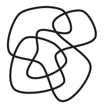 Figure 1
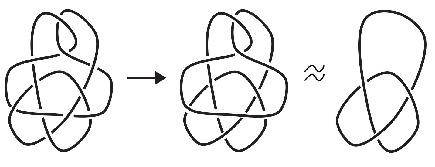 Figure 2
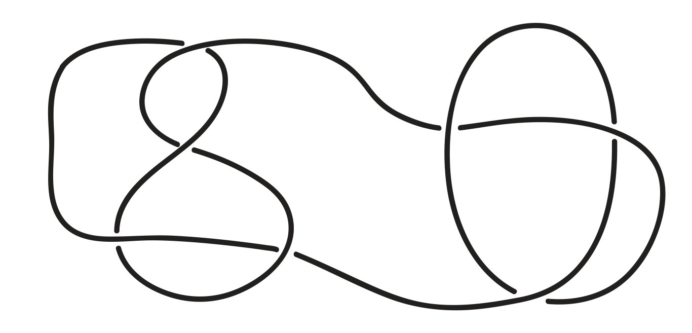 Figure 3
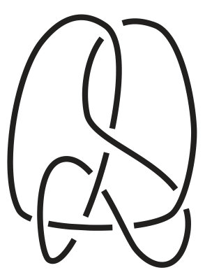 Figure 4
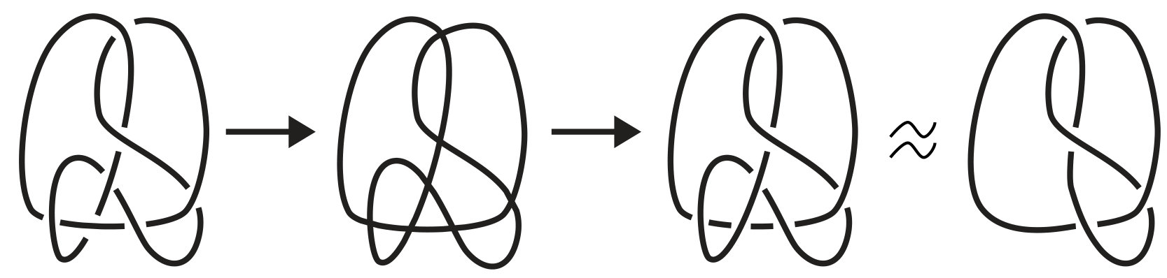 Figure 5
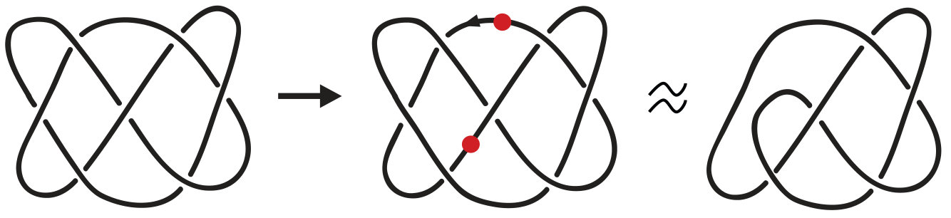 Figure 6
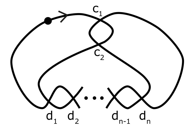 Figure 7
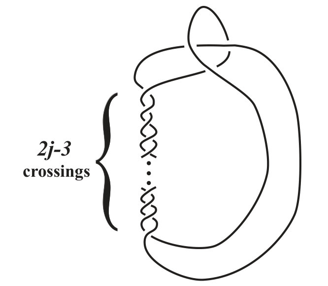 Figure 8
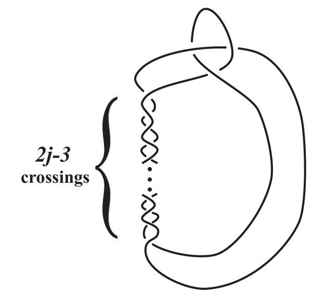 Figure 9
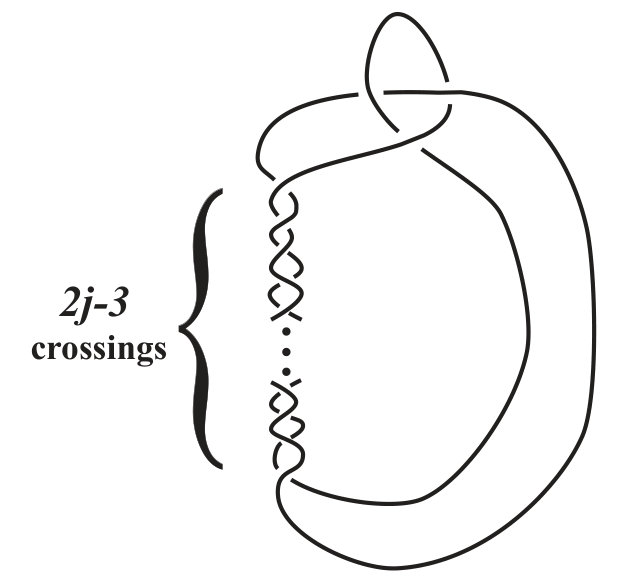 Figure 10
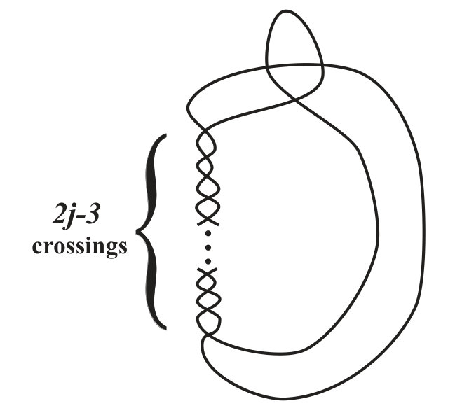 Figure 11
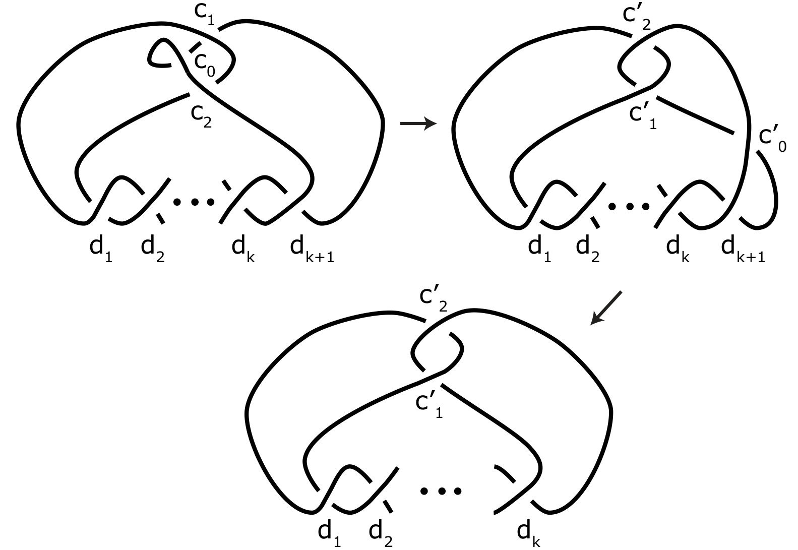 Figure 12
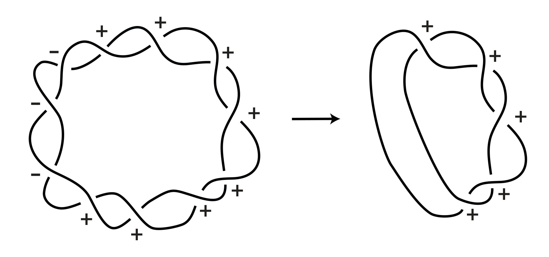 Figure 13
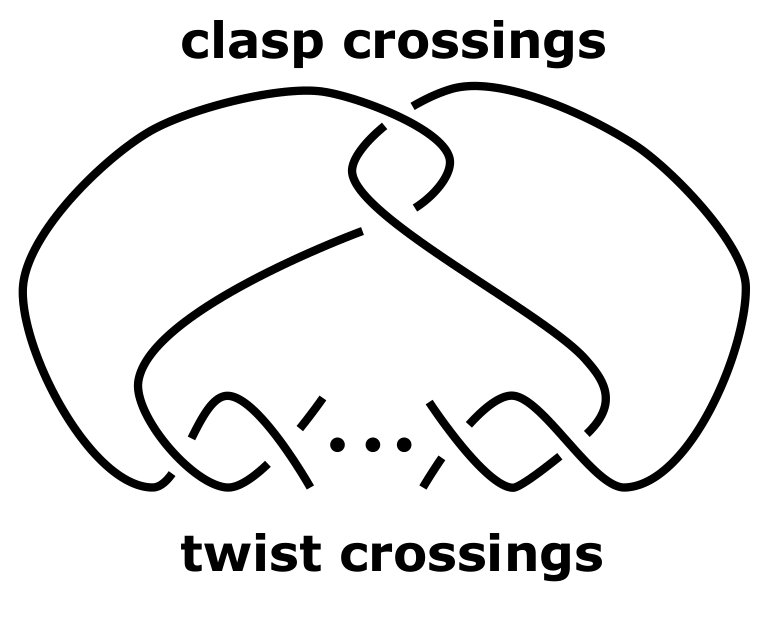 Figure 14
| crossings | shadows | totally unknotted | minimal prime | minimal composite |
|---|---|---|---|---|
| 3 | 6 | 5 | 1 | 0 |
| 4 | 19 | 16 | 1 | 0 |
| 5 | 76 | 55 | 2 | 0 |
| 6 | 376 | 240 | 3 | 2 |
| 7 | 2194 | 1149 | 10 | 3 |
| 8 | 14614 | 6229 | 27 | 13 |
| 9 | 106421 | 35995 | 101 | 59 |
| 10 | 823832 | 219272 | 364 | 263 |
| knot | shadows | knot | shadows | knot | shadows | knot | shadows | knot | shadows |
|---|---|---|---|---|---|---|---|---|---|
| 5 | 13 | 21 | 17 | 2 | |||||
| 7 | 12 | 26 | 18 | 3 | |||||
| 5 | 8 | 27 | 11 | 5 | |||||
| 17 | 7 | 19 | 7 | 10 | |||||
| 14 | 20 | 5 | 19 | 8 | |||||
| 17 | 19 | 16 | 15 | 3 | |||||
| 14 | 14 | 11 | 1 | 3 | |||||
| 8 | 14 | 8 | 2 | 3 | |||||
| 2 | 35 | 13 | 3 | 3 | |||||
| 4 | 32 | 8 | 6 | ||||||
| 2 | 20 | 10 | 6 |
| Knots that are -fertile | |
|---|---|
| 6 | , , , |
| 7 | , |
| 8 | , , , |
| 9 | , |
| 10 | , , , |
| 3 | 3 | 5 | 7 | 6 | 5 | 7 | |||||||
| 4 | 4 | 6 | 6 | 6 | 6 | 7 | |||||||
| 3 | 5 | 6 | 6 | 6 | 6 | 6 | |||||||
| 4 | 5 | 6 | 6 | 7 | 5 | 6 | |||||||
| 4 | 4 | 6 | 6 | 6 | 6 | 6 | |||||||
| 5 | 5 | 6 | 6 | 6 | 6 | 6 | |||||||
| 5 | 6 | 6 | 6 | 6 | 5 | 5 | |||||||
| 3 | 6 | 6 | 6 | 6 | 6 | 6 | |||||||
| 3 | 5 | 6 | 6 | 5 | 6 | 6 | |||||||
| 4 | 5 | 4 | 6 | 5 | 6 | 5 | |||||||
| 5 | 6 | 5 | 6 | 6 | 5 | 6 | |||||||
| 4 | 6 | 5 | 6 | 6 | 6 | 5 | |||||||
| 5 | 6 | 4 | 6 | 6 | 5 | 6 | |||||||
| 6 | 5 | 4 | 7 | 5 | 6 | 5 | |||||||
| 5 | 6 | 3 | 7 | 6 | 6 | 6 | |||||||
| 4 | 5 | 4 | 7 | 6 | 6 | 7 | |||||||
| 4 | 5 | 5 | 7 | 5 | 6 | 6 | |||||||
| 5 | 6 | 4 | 6 | 6 | 5 | 6 | |||||||
| 4 | 6 | 5 | 7 | 6 | 5 | 6 | |||||||
| 5 | 6 | 5 | 7 | 5 | 6 | 6 | |||||||
| 5 | 6 | 6 | 5 | 6 | 6 | 3 | |||||||
| 6 | 6 | 5 | 5 | 6 | 6 | 4 | |||||||
| 5 | 6 | 5 | 5 | 6 | 6 | 5 | |||||||
| 6 | 6 | 5 | 6 | 6 | 6 | 4 | |||||||
| 5 | 6 | 6 | 6 | 6 | 6 | 5 | |||||||
| 5 | 6 | 6 | 6 | 5 | 6 | 6 | |||||||
| 5 | 7 | 6 | 6 | 6 | 6 | 5 | |||||||
| 6 | 6 | 6 | 6 | 6 | 6 | 4 | |||||||
| 6 | 6 | 6 | 6 | 5 | 6 | 5 | |||||||
| 6 | 6 | 6 | 6 | 6 | 6 | 5 | |||||||
| 6 | 6 | 5 | 6 | 6 | 6 | 3 | |||||||
| 5 | 6 | 5 | 6 | 6 | 6 | 5 | |||||||
| 5 | 6 | 6 | 6 | 6 | 6 | 4 | |||||||
| 5 | 6 | 6 | 6 | 5 | 5 | 4 | |||||||
| 5 | 4 | 6 | 6 | 5 | 6 | ||||||||
| 6 | 6 | 5 | 5 | 6 | 6 | ||||||||
| 6 | 5 | 6 | 5 | 6 | 6 | ||||||||
| 3 | 6 | 7 | 6 | 6 | 6 | ||||||||
| 4 | 6 | 6 | 5 | 5 | 6 | ||||||||
| 4 | 5 | 7 | 6 | 6 | 6 |
| knot | siblings |
|---|---|
| 3 | 3 |
|---|
| 4 | 4 | 4 |
| 5 | 5 | 4 | 3 | 4 |
| 6 | 6 | 6 | 5 | 3 | |||||
| 6 | 5 | 4 | 5 |
| 7 | 6 | 6 | 3 | 4 | 5 | ||||||
| 7 | 6 | 6 | 4 | 5 | 4 | ||||||
| 6 | 6 | 4 | 5 | 6 |
| 8 | 7 | 6 | 5 | 6 | 6 | 6 | |||||||
| 8 | 7 | 6 | 4 | 5 | 6 | 6 | |||||||
| 8 | 6 | 6 | 5 | 5 | 5 | 3 | |||||||
| 7 | 5 | 6 | 5 | 5 | 5 | 4 | |||||||
| 8 | 6 | 4 | 6 | 6 | 5 | 4 | |||||||
| 6 | 7 | 4 | 5 | 6 | 5 |
| 9 | 7 | 6 | 4 | 5 | 6 | 6 | |||||||
| 9 | 7 | 7 | 5 | 5 | 6 | 6 | |||||||
| 8 | 6 | 7 | 5 | 6 | 6 | 6 | |||||||
| 8 | 6 | 6 | 4 | 6 | 6 | 6 | |||||||
| 8 | 7 | 6 | 5 | 6 | 6 | 6 | |||||||
| 7 | 6 | 6 | 6 | 6 | 4 | 6 | |||||||
| 7 | 7 | 5 | 6 | 6 | 6 | 4 | |||||||
| 8 | 6 | 6 | 5 | 6 | 5 | 5 | |||||||
| 6 | 7 | 6 | 5 | 6 | 6 | 5 | |||||||
| 7 | 7 | 6 | 6 | 6 | 6 | 4 | |||||||
| 7 | 7 | 5 | 6 | 6 | 5 | 4 | |||||||
| 7 | 6 | 6 | 6 | 7 | 5 | 3 | |||||||
| 7 | 6 | 4 | 5 | 6 | 6 | ||||||||
| 7 | 7 | 3 | 6 | 6 | 6 |
| 10 | 6 | 5 | 7 | 6 | 6 | 6 | |||||||
| 10 | 5 | 6 | 7 | 6 | 5 | 7 | |||||||
| 10 | 6 | 6 | 6 | 6 | 6 | 7 | |||||||
| 9 | 7 | 6 | 6 | 6 | 6 | 6 | |||||||
| 10 | 7 | 6 | 6 | 7 | 5 | 6 | |||||||
| 8 | 6 | 6 | 6 | 6 | 6 | 6 | |||||||
| 9 | 7 | 7 | 6 | 6 | 6 | 6 | |||||||
| 8 | 7 | 6 | 6 | 6 | 5 | 5 | |||||||
| 8 | 7 | 7 | 6 | 6 | 6 | 6 | |||||||
| 8 | 7 | 6 | 6 | 5 | 6 | 6 | |||||||
| 8 | 7 | 6 | 6 | 5 | 6 | 5 | |||||||
| 8 | 7 | 6 | 6 | 6 | 5 | 6 | |||||||
| 8 | 7 | 6 | 6 | 6 | 6 | 5 | |||||||
| 8 | 7 | 5 | 6 | 6 | 5 | 6 | |||||||
| 8 | 7 | 6 | 7 | 5 | 6 | 5 | |||||||
| 8 | 7 | 4 | 7 | 6 | 6 | 6 | |||||||
| 6 | 6 | 4 | 7 | 6 | 6 | 7 | |||||||
| 7 | 7 | 5 | 7 | 5 | 6 | 6 | |||||||
| 7 | 7 | 4 | 6 | 6 | 5 | 6 | |||||||
| 7 | 7 | 5 | 7 | 6 | 5 | 6 | |||||||
| 7 | 7 | 5 | 7 | 5 | 6 | 6 | |||||||
| 7 | 7 | 6 | 5 | 6 | 6 | 3 | |||||||
| 7 | 6 | 5 | 5 | 6 | 6 | 4 | |||||||
| 8 | 7 | 5 | 5 | 6 | 6 | 5 | |||||||
| 8 | 7 | 5 | 6 | 6 | 6 | 4 | |||||||
| 8 | 6 | 6 | 6 | 6 | 6 | 5 | |||||||
| 7 | 7 | 6 | 6 | 5 | 6 | 6 | |||||||
| 7 | 7 | 6 | 6 | 6 | 6 | 5 | |||||||
| 8 | 6 | 6 | 6 | 6 | 6 | 4 | |||||||
| 8 | 6 | 6 | 6 | 5 | 6 | 5 | |||||||
| 8 | 6 | 6 | 6 | 6 | 6 | 5 | |||||||
| 8 | 7 | 5 | 6 | 6 | 6 | 3 | |||||||
| 7 | 6 | 5 | 6 | 6 | 6 | 5 | |||||||
| 7 | 6 | 6 | 6 | 6 | 6 | 4 | |||||||
| 7 | 6 | 6 | 6 | 5 | 5 | 4 | |||||||
| 7 | 6 | 6 | 6 | 5 | 6 | ||||||||
| 8 | 6 | 5 | 5 | 6 | 6 | ||||||||
| 8 | 7 | 6 | 5 | 6 | 6 | ||||||||
| 6 | 6 | 7 | 6 | 6 | 6 | ||||||||
| 6 | 6 | 6 | 5 | 5 | 6 |
Peer Reviews
No public reviews on file for this paper yet. If you reviewed it on a platform where reviews are public (OpenReview, ICLR, NeurIPS, ICML), you can paste yours below so the community can read it here.
Videos
No videos yet. Explain this paper in a talk, walkthrough, or lecture? Add one.
Knot Fertility and Lineage
Jason Cantarella, Allison Henrich, Elsa Magness, Oliver O’Keefe, Kayla Perez,
Eric J. Rawdon and Briana Zimmer
Abstract
In this paper, we introduce a new type of relation between knots called the descendant relation. One knot is a descendant of another knot if can be obtained from a minimal crossing diagram of by some number of crossing changes. We explore properties of the descendant relation and study how certain knots are related, paying particular attention to those knots, called fertile knots, that have a large number of descendants. Furthermore, we provide computational data related to various notions of knot fertility and propose several open questions for future exploration.
1 Introduction
The knot, pictured in Figure 1, is a particularly interesting knot. This is because, in a certain sense, all smaller knots are contained in this knot.
What do we mean by “contained” in this context? We are interested in studying when a knot is a parent of another knot, where parenthood is defined as follows.
Definition 1**.**
A knot is a parent of a knot if a subset of the crossings in a minimal crossing diagram of can be changed to produce a diagram of . In this case, we say that is a descendant of .
For instance, knot is a parent of knot , the trefoil, as shown in Figure 2. Equivalently, we can say that the trefoil is a descendant of . A curious feature of this definition is that any knot is both its own descendant and its own parent.
It is when we consider this more general relationship between knots that we see how interesting is, for is a parent of all knots with strictly smaller crossing number. That is, the descendants of are: , , , , , , , and . It is precisely for this reason that we call a fertile knot.
Definition 2**.**
A knot with crossing number is fertile if is a parent of every knot with crossing number less than .
Now that we have defined the concept of fertility, it is natural to ask, “Which other knots are fertile?” and “Are there any fertile knots with more than seven crossings?” In thinking about the first question, we note that it is a straightforward exercise to verify that , , , , , and are also fertile. In Section 3, we will develop tools to prove that knots such as , , , and are not fertile. The computational results we present in Section 5 illustrate that many other knots with seven or more crossings fail to be fertile. Answering the second question is somewhat trickier. We will introduce the related notions of -fertility and -fertility in Section 4 to reframe this question.
In addition to considering questions that specifically pertain to fertility, we consider more broadly the parent–descendant relationships between knots. For instance, is this relationship transitive? That is, if is a descendant of and is a descendant of , is a descendant of ? We return to this fascinating question in Section 5.
2 Preliminaries
Before we get started, we note that it is often convenient to work with an alternative, but equivalent definition of what it means for one knot to be a parent (or descendant) of another. Suppose is a parent of . Then if we consider all minimal diagrams of and forget these diagrams’ crossing information—so we merely consider their shadows—then must be obtainable by some choice of crossing information in one of these shadows. Figure 3 gives an example of how we derive a descendant from a parent following this process.
We note that a diagram that is missing none, all, or some of its crossing information is referred to as a pseudodiagram, as in [6]. Unknown crossings in a pseudodiagram are called precrossings. Equivalence relations for pseudodiagrams, called pseudo-Reidemeister moves, allow us to think of pseudodiagrams in terms of the knots they have the potential to represent. (See [7] to learn much more about these objects.) Pseudodiagrams and pseudoknots will be useful objects in some constructions in Section 3.
There are a couple of preliminary results we can state now. For instance, we notice that we can equate knots with their mirror images when proving results about knot lineage, on account of the following general fact.
Proposition 3**.**
If a knot is a parent of a knot , then is also a parent of the mirror image of .
Proof.
Let be the shadow corresponding to a minimal diagram of knot , and suppose that is a descendant of . Then we can resolve the precrossings of to produce . Resolving the precrossings of in precisely the opposite way produces a diagram of the mirror image of . So must also be a parent of the mirror image of . ∎
We also make the following observation related to composite knots.
Proposition 4**.**
Suppose that and are either both alternating knots or both torus knots, is a descendant of , and is a descendant of . Then is a descendant of .
Proof.
For a pair of alternating knots and , we know by [10, 14, 16] that forming the connect sum of a minimal diagram of with a minimal diagram of in the plane—as in Figure 4—produces a minimal diagram of . A similar result holds if both and are torus knots by [2]. (We note that, in general, forming the connect sum of two minimal crossing diagrams of factor knots may not produce a minimal diagram of the composite knot [11].) Now, if we resolve a shadow of a minimal diagram of to produce and, likewise, resolve a shadow of a minimal diagram of to produce , these diagrams can be connected to produce a diagram of that projects to the shadow of a minimal diagram of . ∎
Now, without further ado, let us learn about descendant relations in families of knots.
3 Families of Knots
In this section, we consider two key knot families: twist knots and -torus knots. These families distinguish themselves by being closely related to one another—in terms of descendant and parent relations—and rather insular. As a result, we will observe that knots in these families tend to have few descendants.
Keeping this functional equivalence of knots and their mirror images in mind, let us turn to twist knots. A twist knot is a knot formed by two clasp crossings and twist crossings, as in Figure 5. We note that all twist knots are alternating, so it suffices to consider their minimal crossing diagrams as in the figure, where the alternating pattern is preserved as we pass between the clasp crossings and the twist crossings. For these knots, we have the following theorem.
Theorem 5**.**
The knot is a descendant of twist knot if and only if for some integer with .
Proof.
We begin by proving the “only if” direction of Theorem 5. Suppose that the knot is a descendant of twist knot for some positive integer . Then there exists a choice of crossing information for all crossings in the shadow of a standard minimal crossing diagram of (i.e., the shadow of a diagram from Figure 5) that produces a diagram of . Suppose that the clasp crossings, and , have opposite signs in this resolution. Then, is the unknot, . Otherwise, and are alternating.
In the remaining twist crossings, crossings are positive, and crossings are negative. We can perform or (whichever number is smaller) Reidemeister 2 moves to make the twist crossings alternating. If , the result is a two-crossing diagram of the unknot, . Otherwise, some number of twist crossings with the same sign remain. In this case, either the entire knot diagram is alternating, or we can remove one crossing—producing a diagram of —by using the sequence of Reidemeister moves pictured in Figure 6.
To prove the “if” direction of the theorem, let be the shadow of a minimal crossing diagram of , and suppose that is an integer such that . For the remainder of this proof, refer to Figure 7 for orientation and labeling conventions.
Case 1: is even. In the twist of , we resolve the crossings so that half are positive and half are negative. We then perform Reidemeister 2 moves on these crossings to produce the shadow of a minimal crossing diagram of . Finally, we resolve the precrossings in to produce a diagram of .
Case 2: is odd. We resolve the precrossings, in the twist of as in Case 1 so that half of the crossings are positive and half of the crossings are negative. Then, we perform Reidemeister 2 moves to eliminate crossings .
Next, if is odd, we resolve crossings and to be negative and to be positive. If is even, we resolve all of the crossings in the shadow so they are positive. In both cases, the effect of resolving precrossings in this way puts us in the situation of Figure 6 where we obtain a minimal crossing diagram of after a sequence of Reidemeister moves. ∎
Next, we prove a similar result for another knot family: the torus knots, i.e., the knots that can be represented as closures of 2-braids. Note that, since these torus knots are alternating, it suffices to consider their standard minimal diagrams as in, for example, Figure 8.
Theorem 6**.**
The knot is a descendant of torus knot if and only if for some , where and are odd integers.
Proof.
Let be a descendant of torus knot for some positive odd integer . Then, there exists a choice of crossing resolutions that produces a diagram of from the shadow of a minimal crossing diagram of . Suppose there are positive crossing resolutions and negative crossing resolutions for some non-negative integers and . If we let min, we can perform Reidemeister 2 moves to reduce the number of crossings in the diagram by . The resulting knot is .
To prove the converse, we consider the torus knot where is a positive odd integer, and we let be a positive odd integer less than . In the shadow of , we resolve crossings to be positive and the remaining crossings to be negative. This enables us to perform Reidemeister 2 moves—as in the Figure 8 example—to obtain a minimal crossing diagram of . ∎
4 Notions of Fertility
As we mentioned in the introduction, , , , , , , and are all fertile knots. On the other hand, the results of Section 2 allow us to show that knots , , , and are not fertile. Indeed, the knot is and is , while the figure-eight knot, does not equal for any , so fails to be a descendant of either knot. Furthermore, and are both twist knots while is not a twist knot and, hence, not a descendant. So both and fail to be fertile. A fun afternoon exercise shows that all other knots with seven or fewer crossings—namely, , , , and —fail to be fertile. For instance, we can show that is not a descendant of or while is not a descendant of or .
What about prime knots with more than seven crossings? What about composite knots? Computations for all prime and composite knots with 10 or fewer crossings reveals that there are no 8-, 9-, or 10-crossing fertile knots. In fact, we conjecture that there are no fertile knots with crossing number greater than seven.
So, is fertility a helpful notion? Yes and no. To gain insights about a knot’s structure from the notion of fertility, we expand our definition.
Definition 7**.**
A knot is n-fertile if it is a parent of every knot with or fewer crossings.
In other words, if a knot is -fertile and has crossing number , then is fertile. But for every knot , there is some nonnegative integer for which is -fertile. This notion enables us to define a new knot invariant.
Definition 8**.**
The fertility number, , of a knot is the greatest integer for which is -fertile.
What do we already know about the fertility number? First, the maximum value of for a knot with crossing number is . (Notice that the figure-eight knot is 4-fertile, the trefoil is 3-fertile, and the unknot is 0-fertile.) Furthermore, 0 is clearly a lower bound for , but perhaps we can say more. In Section 6, we will discuss how to improve the lower bound of in general. For small knots, the results in Section 5 will tell us so much more.
Before we look at fertility numbers for specific knots, we introduce one more notion related to knot fertility called -fertility.
Definition 9**.**
A knot is (n,m)-fertile if for each prime knot with , there is a knot shadow (not necessarily from a minimal diagram) with crossings that contains both and .
To determine if a knot is -fertile, one searches through all -crossing shadows that have as a resolution. (For instance, if , then this set of shadows is just all shadows coming from minimal diagrams of .) If the union of the resolution sets of all these shadows contains all knots with or fewer crossings, then is -fertile.
One of the first things we notice from Definition 9 is that -fertility is equivalent to fertility for crossing knots. We explore the concept of -fertility further in Sections 5 and 6.
5 Computational Results
Cantarella et al. [1] have computed an exhaustive list of all knot shadows through 10 crossings. By assigning all possible crossings to these shadows and analyzing all knot types resulting from the resulting knot diagrams, we obtain complete information about knot fertility for knots through 10 crossings.
The knot types were computed using lmpoly, a program by Ewing and Millett [4] to compute the HOMFLYPT polynomial [5] of diagrams, and knotfind, a program to compute knot types from Dowker codes, which is a part of the larger program Knotscape by Hoste and Thistlethwaite [8]. The program knotfind does not distinguish between the different chiralities of chiral knots. Since fertility is a non-chiral property (see Prop. 3), knotfind would have been sufficient for the work here. However, we used the HOMFLYPT computation via lmpoly as a further check on the data.
In Table 1, we show for each crossing number the total number of shadows, the number of shadows which host only unknots (which we call totally unknotted), and the number of shadows which yield a minimal crossing diagram (partitioned into prime and composite knot shadows). Note that some shadows host minimal diagrams for multiple knot types. In the table, the number of minimal diagrams are counted without multiplicity.
When different minimal diagrams exist for alternating knot types, they are all related by flype moves [9]. Thus, the list of descendants derived from one minimal diagram of an alternating knot is precisely the same as the list derived from any other minimal diagram. Minimal diagrams of non-alternating knot types, though, need not be related by flype moves. As a result, the lists of descendants derived from different minimal diagrams of a non-alternating knot might differ. In our fertility table, Table 5, we considered a knot type to be a descendant of a non-alternating knot type if there exists a shadow containing crossings that has both and as resolutions. This is consistent with—though it represents a different way of viewing—our original definition of “descendant.”
To give the reader some idea of the computational complexity of this problem, we provide Table 2, which shows the number of minimal diagrams for non-alternating knot types through 10 crossings.
In Table 5, we record fertility numbers, which provide one sort of summary of our more significant computational results. In fact, we derived an exhaustive list of descendants of all knots with up to 10 crossings. This collection of data is too vast to share here, but we can share some interesting observations we derived from the data.
First, and perhaps most interestingly, we found the descendant relation is decidedly not transitive. There are a number of counterexamples to transitivity, most of which involve non-alternating knot types. However, there are nine examples of non-transitivity involving only alternating knot types through 10 crossings. See Table 3.
The use of the term “descendant” in this paper leads to other strange naming conventions for knot relationships. In particular, we call a knot a sibling of a knot , where , if there is an -crossing shadow that has both and as resolutions.111The term “sibling” was used in a similar context in [3], though the two definitions differ. Note that for a given shadow, there are only two ways of assigning crossings to yield an alternating diagram, and these two diagrams are mirror images. Thus, these sibling relationships only occur between alternating and non-alternating or non-alternating and non-alternating knot types. Table 6 shows all sibling relationships for 8- and 9-crossing knot types. We created a table of sibling relationships between 10-crossing knots, but it is too unwieldy to include here. For instance, alone has 41 siblings!
Another interesting aspect of -fertility that can be studied is a notion of anti-fertility. Specifically, which knots act as roadblocks to more complex knots achieving -fertility for various values of ? For instance, our computations show that the knots , , and fail to be descendants of 15 of the 18 alternating 8-crossing knots. In essence, these three knots are providing a significant barrier to 8-crossing knots achieving fertility. These three knots continue to be problematic for alternating knots with crossing number 9 or 10. Of the 41 alternating 9-crossing knots, fails to be a descendant of 31 knots, fails to be a descendant of 26 knots, and fails to be a descendant of 19 knots. Similarly, of the 123 alternating 10-crossing knots, fails to be a descendant of 77 knots, fails to be a descendant of 67 knots, and fails to be a descendant of 53 knots.
Consider another unusual example. If we examine the shadows of alternating 9-crossing knots, we find that and fail to appear in the resolution sets of of 40 of the 41 representative shadows.222Note that we are only considering the shadow of one representative from each equivalence class of reduced, alternating knot diagrams that are related by flypes. In other words, and are each only descendants of one alternating 9-crossing knot ( and , respectively). The knot provides another barrier to fertility for 9- and 10-crossing knots. It fails to be a descendant of 38 out of 41 alternating 9-crossing knots and 109 of 123 alternating 10-crossing knots.
Just as we can make a number of observations about -fertility and anti-fertility, the data set helps us compute -fertility numbers for a number of knots. See Tables 7-14 in the appendix for a complete list of -fertility numbers for knots with up to 10 crossings. We highlight a subset of this data here, namely examples of knots that are -fertile for some . Table 4 shows a complete list of -fertile knots for . It is no surprise that the unknot is fertile for each since every knot shadow can be resolved to produce a diagram of the unknot. More interestingly, we notice that , , and are -fertile for certain values, following regular patterns. Using the observations of Table 4 and the results of Section 6, we are able to prove that these patterns hold ad infinitum.
There are likely many more interesting observations that can be made from staring at our data, but for now, we move on to discussing how our work fits in the context of the work done by others over the years.
6 Other Knot Relations
Our notion of descendant is not the first notion that attempts to capture what it means for a knot to contain another knot. For instance, the descendant relation shares some similarities with the notion of predecessor, introduced in [3].
Definition 10**.**
A knot is a predecessor of knot if the crossing number of is less than that of and can be obtained from a minimal diagram of by a single crossing change.
We see that, while the trefoil is a descendant of the figure-eight knot, it is not a predecessor since two crossing changes are required to derive a trefoil from a minimal diagram of the figure-eight knot. So if a knot is a predecessor of a knot , then is a descendant of , but the converse fails to hold in general.
In another effort to relate knots to their parts, Millett and Jablan described what it means for one knot to be a subknot of another knot [13]. In particular, they gave the following definition.
Definition 11**.**
A knot is a subknot of knot if it can be obtained from a minimal diagram of by crossing changes that preserve those within a segment of the diagram and change those outside this segment so that the complementary segment is strictly ascending.
In Figure 9, we see that the twist knot is a subknot of . Indeed, if crossing changes are performed on a segment of the knot between the two dots so that this segment is ascending, we find that knot is produced.
While the subknot definition seems stricter than the descendant relation, is it possible that the subknot and descendant relations are actually the same relations in disguise? Just as with the predecessor relation, we immediately observe that if a knot is a subknot of knot , then is a descendant of . What about the converse? In [12], it was proven that the trefoil is not a subknot of . On the other hand, we illustrated in Figure 2 that the trefoil is a descendant of , so the descendant and subknot relations must be distinct.
Finally, another well-known relationship between knots is one that was introduced by Taniyama in [15].
Definition 12**.**
A knot is a minor of knot if the set of knot shadows that have as a resolution is a subset of the set of shadows that have as a resolution.
Once again, we notice that if is a minor of , then is a descendant of . Since all shadows of diagrams of are also shadows of diagrams of when is a minor of , then in particular, a minimal crossing shadow of will have as a resolution. To determine if the minor relation is the same as the descendant relation, we need to ask about the converse. Our results from Section 5 hold the key to answering this question. Our computations show that is a descendant of . We also know that is a descendant of , but is not a descendant of —in fact, this trio of knots is one of our counterexamples to transitivity. More concretely, the shadow in Figure 10 contains but not . So is not a minor of . This proves that the descendant and minor relations are distinct.
While the descendant and minor relations are interestingly different, the fact that if is a minor of , then is a descendant of yields the following result as a corollary of Theorem 1 in [15].
Corollary 13**.**
Every nontrivial knot has the trefoil as a descendant.
From this result, we see in particular that the fertility number for any nontrivial knot must be at least 3. We can also infer the following result.
Theorem 14**.**
The trefoil is -fertile for all .
Similarly, we have the following three corollaries of Theorems 2, 3, and 4 in [15]. Each of these corollaries has further implications for bounds on fertility numbers.
Corollary 15**.**
If has a prime factor that is not equivalent to a -torus knot with , then has the figure-eight knot as a descendant.
Corollary 16**.**
If has a prime factor that is not equivalent to a -torus knot with or the figure-eight knot, then has the knot as a descendant.
Corollary 17**.**
If has a prime factor that is not equivalent to any of the pretzel knots (where , , and are odd integers), then has the knot as a descendant.
Corollaries 15 and 16 have a particularly nice consequence for -fertility that puts the data in Table 4 into a larger context. We can use these corollaries to prove the following result.
Theorem 18**.**
The figure-eight knot, , and the twist knot, , are both -fertile for any integer .
Proof.
Let us fix an integer . Our goal is to show: for every prime knot with crossing number less than or equal to , there is a knot shadow with crossings that has (resp. ) as a descendant. We prove the result for . The proof for is similar.
Let be any knot with . By Corollary 15, the only prime knots that fail to have as a descendant are torus knots.
Case 1: is not a torus knot. We know that is a descendant of , i.e. there is a -crossing shadow that can be resolved to both and . If , then we are done. If , then we can add crossings by applying pseudo-R1 moves to to obtain a -crossing shadow which resolves to both and .
Case 2: is a torus knot. In Figure 11, we provide a -crossing shadow that can be resolved to produce , , and all torus knots with odd, , which suffices to prove the theorem. We illustrate in subdiagram (b) that the torus knot can be derived from the shadow pictured in (a). By an argument similar to the one that proved Theorem 6, we can also derive from this shadow every torus knot with , where is an odd integer. Subdiagrams (c) and (d) illustrate our desired resolutions of the and knots, respectively. ∎
7 Conclusion
We conclude with some of our favorite lingering questions and ideas.
Are there fertile knots with crossing number greater than seven?
It seems highly unlikely that, if there are no fertile knots with crossing number 8, 9, or 10, there will suddenly appear a fertile knot with crossing number greater than 10. We have not conclusively ruled this possibility out, however. How could one prove that no more fertile knots exist? 2. 2.
Can the results of Section 3 be generalized? In other words, what more can we say about our favorite families of knots?
We have yet to explore other families of rational knots, pretzel knots, or Montesinos knots. In general, are there similar descendant relationships between families of knots other than twist knots and torus knots? 3. 3.
For an arbitrary -crossing knot , what proportion of -crossing knots (where ) should we expect to be parents of ?
For example, each alternating 8-crossing knot fails to be a descendant of between 33 and 41 of the 9-crossing alternating knots. In other words, each alternating 8-crossing knot has at most eight 9-crossing parents. Of the 123 10-crossing alternating knots, any given alternating 8-crossing knot will fail to be a descendant of between 73 and 116. 4. 4.
What more can we say about barriers to fertility?
For instance, for a given , what is the smallest set, , of alternating -crossing knots which has the property that no alternating -crossing knot has all members of as descendants? 5. 5.
What more can we say about -fertility in general and -fertility in particular?
We saw that , , and are -fertile for infinitely many . Are there other knot types that are -fertile for all sufficiently large or all sufficiently large odd or even ?
Acknowledgments
First, we would like to thank Ken Millett, Erica Flapan, Claus Ernst, Harrison Chapman, and Colin Adams for their suggestions that led to improvements of this paper. We express our deep gratitude to the National Science Foundation for supporting this work through grants DMS #1460537 and #1418869. This work was also supported by a grant from the Simons Foundation (#426566, Allison Henrich) as well as the Clare Boothe Luce Foundation and the Seattle University College of Science and Engineering. Finally, this project was inspired by an observation of Inga Johnson’s. We thank her for the inspiration.
The reference list from the paper itself. Each links out to its DOI / PubMed record.
- 1[1] Jason Cantarella, Harrison Chapman, and Matt Mastin. Knot probabilities in random diagrams. J. Phys. A , 49(40):405001, 28, 2016.
- 2[2] Yuanan Diao. The additivity of crossing numbers. J. Knot Theory Ramifications , 13(07):857–866, 2004.
- 3[3] Yuanan Diao, Claus Ernst, and Andrzej Stasiak. A partial ordering of knots through diagrammatic unknotting. J. Knot Theory Ramifications , 18(4):505–522, 2009.
- 4[4] Bruce Ewing and Kenneth C. Millett. Computational algorithms and the complexity of link polynomials. In Progress in knot theory and related topics , pages 51–68. Hermann, Paris, 1997.
- 5[5] P. Freyd, D. Yetter, J. Hoste, W. B. R. Lickorish, K. Millett, and A. Ocneanu. A new polynomial invariant of knots and links. Bull. Amer. Math. Soc. (N.S.) , 12(2):239–246, 1985.
- 6[6] Ryo Hanaki. Pseudo diagrams of knots, links and spatial graphs. Osaka J. Math. , 47(3):863–883, 2010.
- 7[7] Allison Henrich, Rebecca Hoberg, Slavik Jablan, Lee Johnson, Elizabeth Minten, and Ljiljana Radović. The theory of pseudoknots. J. Knot Theory Ramifications , 22(7):1350032, 21, 2013.
- 8[8] Jim Hoste and Morwen Thistlethwaite. Knotscape. http://www.math.utk.edu/ ∼ similar-to \sim morwen/knotscape.html, 2009. Program for computing topological information about knots.