The Dual Graph Shift Operator: Identifying the Support of the Frequency Domain
Geert Leus, Santiago Segarra, Alejandro Ribeiro, Antonio G. Marques

TL;DR
This paper introduces the dual graph shift operator to better interpret the support of graph frequency signals, enabling improved analysis, filtering, and understanding of graph-structured data.
Contribution
It proposes the dual GSO, a novel concept that captures the support of graph frequency signals as a graph, enhancing interpretability and processing in graph signal analysis.
Findings
Dual GSO provides a richer interpretation of graph frequency support.
Enables development of improved graph filters and filter banks.
Facilitates generalization of classical signal processing results to graphs.
Abstract
Contemporary data is often supported by an irregular structure, which can be conveniently captured by a graph. Accounting for this graph support is crucial to analyze the data, leading to an area known as graph signal processing (GSP). The two most important tools in GSP are the graph shift operator (GSO), which is a sparse matrix accounting for the topology of the graph, and the graph Fourier transform (GFT), which maps graph signals into a frequency domain spanned by a number of graph-related Fourier-like basis vectors. This alternative representation of a graph signal is denominated the graph frequency signal. Several attempts have been undertaken in order to interpret the support of this graph frequency signal, but they all resulted in a one-dimensional interpretation. However, if the support of the original signal is captured by a graph, why would the graph frequency signal have a…
Click any figure to enlarge with its caption.
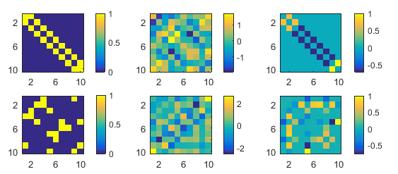 Figure 1
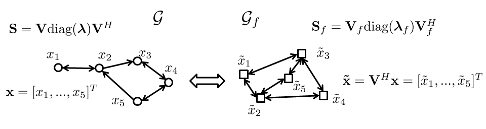 Figure 2
Peer Reviews
No public reviews on file for this paper yet. If you reviewed it on a platform where reviews are public (OpenReview, ICLR, NeurIPS, ICML), you can paste yours below so the community can read it here.
Videos
No videos yet. Explain this paper in a talk, walkthrough, or lecture? Add one.
The Dual Graph Shift Operator: Identifying the Support of the Frequency Domain
Geert Leus, , Santiago Segarra, , Alejandro Ribeiro, ,
and Antonio G. Marques Work in this paper is supported by Spanish MINECO grants No TEC2013- 41604-R, TEC2016-75361-R and USA NSF CCF-1217963. G. Leus is with the Dept. of Electrical Eng., Math. and Comp. Science, Delft Univ. of Technology. S. Segarra is with the Inst. for Data, Systems and Society, Massachusetts Inst. of Technology. A. Ribeiro are with the Dept. of Electrical and Systems Eng., Univ. of Pennsylvania. A. G. Marques is with the Dept. of Signal Theory and Comms., King Juan Carlos Univ. Emails: [email protected], [email protected], [email protected], [email protected].
Abstract
Contemporary data is often supported by an irregular structure, which can be conveniently captured by a graph. Accounting for this graph support is crucial to analyze the data, leading to an area known as graph signal processing (GSP). The two most important tools in GSP are the graph shift operator (GSO), which is a sparse matrix accounting for the topology of the graph, and the graph Fourier transform (GFT), which maps graph signals into a frequency domain spanned by a number of graph-related Fourier-like basis vectors. This alternative representation of a graph signal is denominated the graph frequency signal. Several attempts have been undertaken in order to interpret the support of this graph frequency signal, but they all resulted in a one-dimensional interpretation. However, if the support of the original signal is captured by a graph, why would the graph frequency signal have a simple one-dimensional support? That is why, for the first time, we propose an irregular support for the graph frequency signal, which we coin the dual graph. The dual GSO leads to a better interpretation of the graph frequency signal and its domain, helps to understand how the different graph frequencies are related and clustered, enables the development of better graph filters and filter banks, and facilitates the generalization of classical SP results to the graph domain.
Index Terms:
Graph signal processing, Dual graph shift operator, Frequency support, Graph Fourier transform, Duality.
I Introduction
Graph signal processing (GSP) has emerged as an effective solution to handle data with an irregular support. Its approach is to represent this support by a graph, view the data as a signal defined on its nodes, and use algebraic and spectral properties of the graph to study the signals [1]. Such a data structure appears in many domains, including social networks, smart grids, sensor networks, and neuroscience. Instrumental to GSP are the notions of the graph shift operator (GSO), which is a matrix that accounts for the topology of the graph, and the graph Fourier transform (GFT), which allows the representation of graph signals in the so-called graph frequency domain. These tools are the fundamental building blocks for the development of compression schemes, filter banks, node-varying filters, windows, and other GSP techniques [2, 3, 4, 5, 6, 7, 8].
Motivated by the practical importance of the GFT, some efforts have been made to establish a total ordering of the graph frequencies [1, 9, 10], implicitly assuming a one-dimensional support for the graph frequency signal. Such an ordering translates into proximities between frequencies, which are critical for the definition of bandlimitedness and smoothness as well as for the design of sampling and (bank) filtering schemes. However, the basis vectors associated with frequencies that are close in such one-dimensional domains are often dissimilar and focus on completely different parts of the graph [11], suggesting that a one-dimensional support is not descriptive enough to capture the similarity relationships between graph frequencies. To overcome that limitation, we propose the first description of the (not necessarily regular) support of a graph frequency signal by means of a graph (which we denominate as the dual graph111This is not related to the graph theoretic notion of dual graph of a planar graph , which is a graph that has a vertex for each face of [12].) and its corresponding dual GSO. This dual GSO helps in describing the existing relations across frequencies, which can be ultimately leveraged to enhance existing vertex-frequency GSP schemes.
II The dual graph
We start by reviewing fundamental concepts of GSP and then state formally the problem of identifying the dual GSO.
II-A Fundamentals of GSP
Consider a graph of nodes or vertices with node set and edge set {\mathcal{E}}=\{(n_{i},n_{j})\,|\,\text{n_{i}n_{j}}\}. The graph is further characterized by the so-called GSO, which is an matrix whose entries for are zero whenever nodes and are not connected. The diagonal entries of can be selected freely and typical choices for the GSO include the Laplacian or adjacency matrices [1, 9]. A graph signal defined on can be conveniently represented by a vector , where is the signal value associated with node .
The GSO – encoding the structure of the graph – is crucial to define the GFT and graph filters. The former transforms graph signals into a frequency domain, whereas the latter represents a class of local linear operators between graph signals. Assume for simplicity that the GSO is normal, such that its eigenvalue decomposition (EVD) can always be written as {\mathbf{S}}={\mathbf{V}}{\mbox{\boldmath\Lambda}}{\mathbf{V}}^{H}, where is a unitary matrix that stacks the eigenvectors and is a diagonal matrix that stacks the eigenvalues. To simplify exposition, we also assume the eigenvalues of the shift are simple (non-repeated), such that the associated eigenspaces are unidimensional. The eigenvectors correspond to the graph frequency basis vectors whereas the eigenvalues {\mbox{\boldmath\lambda}}=\text{diag}({\mbox{\boldmath\Lambda}})=[\lambda_{1},...,\lambda_{N}]^{T} can be viewed as graph frequencies. With these conventions, the definitions of the GFT and graph filters are given next.
Definition 1**.**
*Given the GSO {\mathbf{S}}={\mathbf{V}}{\mbox{\boldmath\Lambda}}{\mathbf{V}}^{H}, the GFT of the graph signal is . *
Definition 2**.**
Given the GSO {\mathbf{S}}={\mathbf{V}}{\mbox{\boldmath\Lambda}}{\mathbf{V}}^{H}, a graph filter of degree is a graph-signal operator of the form
[TABLE]
where and {\tilde{\mathbf{h}}}:=\text{diag}(\sum_{l=0}^{L}h_{l}{\mbox{\boldmath\Lambda}}^{l}).
Definition 1 implies that the inverse GFT (iGFT) is simply . Vector in Definition 2 collects the filter coefficients and in (2) can be deemed as the frequency response of the filter. The particular case of the filter being , so that {\tilde{\mathbf{h}}}={\mbox{\boldmath\lambda}}, will be subject of further discussion in Section III. Graph filters and the GFT have been shown useful for sampling, compression, filtering, windowing, and spectral estimation of graph signals [2, 3, 4, 5, 6, 7, 8].
II-B Support of the frequency domain
The underlying assumption in GSP is that to analyze and process the graph signal one has to take into account its graph support via the associated GSO . Moreover, according to Definition 1 the graph frequency signal is an alternative representation of . Thus, a natural problem is the identification of the graph and the GSO corresponding to . More precisely, we are interested in finding the dual graph – represented via the corresponding dual GSO – that characterizes the support of the frequency domain.
Let denote the node set of the dual graph . Each element in corresponds to a different frequency , thus, the edge set indicates pairwise relations between the different frequencies. We interpret as a signal defined on this dual graph, where is associated with the node (frequency) . As for the primal GSO, the EVD of the matrix associated with will be instrumental to study . We start from the assumption that normality of implies normality of . Later on, we will see that this assumption is valid. Due to normality, we have then that {\mathbf{S}}_{f}={\mathbf{V}}_{f}{\mbox{\boldmath\Lambda}}_{f}{\mathbf{V}}^{H}_{f}, and thus the dual graph has (dual) frequency basis vectors and (dual) graph frequencies {\mbox{\boldmath\lambda}}_{f}=\text{diag}({\mbox{\boldmath\Lambda}}_{f})=[\lambda_{f,1},...,\lambda_{f,N}]^{T} (cf. Fig. 1).
Problem statement. Given the GSO {\mathbf{S}}={\mathbf{V}}{\mbox{\boldmath\Lambda}}{\mathbf{V}}^{H} find the dual GSO {\mathbf{S}}_{f}={\mathbf{V}}_{f}{\mbox{\boldmath\Lambda}}_{f}{\mathbf{V}}^{H}_{f}.
To address this problem we postulate desirable properties that we want the dual GSO to satisfy. First, we start by identifying (Section III). We then proceed to determine {\mbox{\boldmath\Lambda}}_{f} (Section IV), which is a more challenging problem.
III Eigenvectors of the dual graph
We want the GFT associated with the dual graph to map back to graph signal . Given that (cf. Definition 1), the ensuing result follows.
Property 1**.**
Given the primal GSO {\mathbf{S}}={\mathbf{V}}{\mbox{\boldmath\Lambda}}{\mathbf{V}}^{H}, the eigenvectors of the dual GSO are .
As announced in the previous section, since we have that , then the dual shift is normal too. With denoting the th canonical basis vector (all entries are zero except for the one corresponding to the th node, which is one), then can be written as , i.e., the GFT of the graph signal . Hence, the dual frequency vector can be viewed as how node expresses each of the primal graph frequencies, revealing that each frequency of the dual graph is related to a particular node of the primal graph . Moreover, we can also interpret the dual eigenvalues from a primal perspective. To that end, note that {\mbox{\boldmath\lambda}}_{f} is the frequency response of the dual filter (cf. discussion after Definition 2); thus, the th entry of {\mbox{\boldmath\lambda}}_{f} can be understood as how strongly the primal value at the th node is amplified when is applied to .
One interesting implication of Property 1 is that the dual of a Laplacian shift {\mathbf{S}}={\mathbf{V}}{\mbox{\boldmath\Lambda}}{\mathbf{V}}^{H} is, in general, not a Laplacian. Laplacian matrices require the existence of a constant eigenvector. Hence, for to be a Laplacian, one of the rows of – corresponding to the columns of – needs to be constant, which in general is not the case. Another implication of Property 1 is the duality of the filtering and windowing operations, as shown next.
Corollary 1**.**
Given the graph signal and the window , define the windowed graph signal as
[TABLE]
Then, recalling that and , if does not have repeated eigenvalues it holds that
[TABLE]
for some and .
**Proof: ** Substituting and into the definition of yields . This reveals that the mapping from to is given by the matrix . Since is normal and unitary, are the eigenvectors of and are its eigenvalues. Because are also the eigenvectors of (cf. Property 1), to show that is a filter on we only need to show that there exist coefficients such that {\mathbf{w}}=\text{diag}(\sum_{l=0}^{N-1}h_{f,l}{\mbox{\boldmath\Lambda}}_{f}^{l}) [cf. (1)]. Defining {\mbox{\boldmath\Psi}}_{f}\in\mathbb{C}^{N\times N} as [{\mbox{\boldmath\Psi}}_{f}]_{i,l}=(\lambda_{f,i})^{l-1}, the equality can be written as {\mathbf{w}}={\mbox{\boldmath\Psi}}_{f}{\mathbf{h}}_{f}. Since {\mbox{\boldmath\Psi}}_{f} is Vandermonde, if all the dual eigenvalues are distinct, an solving {\mathbf{w}}={\mbox{\boldmath\Psi}}_{f}{\mathbf{h}}_{f} exists.
The proof holds regardless of the particular {\mbox{\boldmath\lambda}}_{f} and only requires to have non-repeated eigenvalues. The corollary states that multiplication in the vertex domain is equivalent to filtering in the dual domain – note that the GSO of the filter in (3) is . Clearly, when the entries of are binary values, multiplying by acts as a windowing procedure preserving the values of in the support , while discarding the information at the remaining nodes.
IV Eigenvalues of the dual graph
Given {\mathbf{S}}={\mathbf{V}}\text{diag}({\mbox{\boldmath\lambda}}){\mathbf{V}}^{H} and using Property 1 to write the dual shift as {\mathbf{S}}_{f}={\mathbf{V}}^{H}\text{diag}({\mbox{\boldmath\lambda}}_{f}){\mathbf{V}}, the last step to identify is to obtain {\mbox{\boldmath\lambda}}_{f}. Two different (complementary) approaches to accomplish this are discussed next.
IV-A Axiomatic approach
Our first approach is to postulate properties that we want the dual shift to satisfy, and then translate these properties into requirements on the dual eigenvalues {\mbox{\boldmath\lambda}}_{f}. We denominate these properties as axioms, which we state next. In the following, denotes an arbitrary permutation matrix.
(A1) Axiom of Duality. The dual of the dual graph is equal to the original graph
[TABLE]
(A2) Axiom of Reordering. The dual graph is robust to reordering the nodes in the primal graph
[TABLE]
(A3) Axiom of Permutation. Permutations in the EVD of the primal shift lead to permutations in the dual graph
[TABLE]
Consistency with Property 1 is encoded in the Axiom of Duality (A1). More precisely, since the GFT of the dual shift transforms a frequency signal back into the graph domain , we want the associated shift to be recovered as well.The Axiom of Reordering (A2) ensures that the frequency structure encoded in the dual shift is invariant to relabelings of the nodes in the primal shift. Specifically, the frequency coefficients of a given signal with respect to should be the same as those of with respect to . Finally, since the nodes of the dual graph correspond to different frequencies, the Axiom of Permutation (A3) ensures that if we permute the eigenvectors (and corresponding eigenvalues) of , the nodes of the dual shift are permuted accordingly.
Axioms (A1)-(A3) impose conditions on the possible choices for the dual eigenvalues {\mbox{\boldmath\lambda}}_{f}. More precisely, let us define the function , that computes the dual eigenvalues {\mbox{\boldmath\lambda}}_{f}=h({\mbox{\boldmath\lambda}},{\mathbf{V}}) as a function of the eigen-decomposition of . In terms of , axiom (A1) requires that
[TABLE]
In order to translate (5) into a condition on , notice that {\mathbf{P}}{\mathbf{S}}{\mathbf{P}}^{T}={\mathbf{P}}{\mathbf{V}}\text{diag}({\mbox{\boldmath\lambda}}){\mathbf{V}}^{H}{\mathbf{P}}^{T} so that from Property 1 must be equal to {\mathbf{V}}^{H}{\mathbf{P}}^{T}\text{diag}({\mbox{\boldmath\lambda}}^{\prime}){\mathbf{P}}{\mathbf{V}}. Thus, for to coincide with we need {\mbox{\boldmath\lambda}}^{\prime}={\mathbf{P}}{\mbox{\boldmath\lambda}}_{f} which ultimately requires that
[TABLE]
Lastly, in order to find the requirement imposed by axiom (A3) on , we again leverage Property 1 to obtain ({\mathbf{V}}{\mathbf{P}}\text{diag}({\mathbf{P}}^{T}{\mbox{\boldmath\lambda}}){\mathbf{P}}^{T}{\mathbf{V}}^{H})_{f}={\mathbf{P}}^{T}{\mathbf{V}}^{H}\text{diag}({\mbox{\boldmath\lambda}}^{\prime}){\mathbf{V}}{\mathbf{P}}. It readily follows that to satisfy (6) we need {\mbox{\boldmath\lambda}}^{\prime}={\mbox{\boldmath\lambda}}_{f}, i.e.
[TABLE]
It is possible to find a function that simultaneously satisfies (7)-(9), as shown next.
Theorem 1**.**
The following class of functions satisfies (7)-(9), leading to a generating method for dual graphs that abides by axioms (A1)-(A3)
[TABLE]
where and , with any permutation invariant function, i.e., .
**Proof: ** We show that (10) satisfies (7), (8), and (9). Showing that (7) holds, requires only substituting (10) into h(h({\mbox{\boldmath\lambda}},{\mathbf{V}}),{\mathbf{V}}^{H}), which yields
[TABLE]
In order to show (8), notice that a permutation of the rows of (the columns of ) does not influence and only permutes the diagonal entries of . Hence, we can write h({\mbox{\boldmath\lambda}},{\mathbf{P}}{\mathbf{V}}) as
[TABLE]
Finally, since a permutation of the columns of (the rows of ) does not influence and only permutes the diagonal entries of , we can write h({\mathbf{P}}^{T}{\mbox{\boldmath\lambda}},{\mathbf{V}}{\mathbf{P}}) as [cf. (9)]
[TABLE]
Note that Theorem 1 proves the existence of a class of eligible dual graphs, but it does not indicate that every dual graph falls in this class. If we restrict ourselves to the class in (10), which can be described by the function , the simplest choice for is . This results in {\mbox{\boldmath\lambda}}_{f}={\mathbf{V}}{\mbox{\boldmath\lambda}}, but any power of any norm is also a valid function, i.e., . A possible policy to design a dual graph could be to select the function that optimizes a particular figure of merit (such as the minimization of the number of edges in the dual graph ) yet keeping faithful to (A1)-(A3). This problem is discussed in more detail at the end of the following section. Furthermore, additional axioms can be imposed on to further winnow the class of admissible functions . A possible avenue, not investigated here, is to impose a desirable behavior of with respect to the intrinsic phase ambiguity of the primal EVD.
IV-B Optimization approach
A different (and complementary) approach is to find a dual shift for which certain properties of practical relevance are promoted. For example, one may be interested in the sparsest . To be rigorous, consider that the primal shift {\mathbf{S}}={\mathbf{V}}{\mbox{\boldmath\Lambda}}{\mathbf{V}}^{H} is given. Then, upon setting (cf. Property 1), the dual shift is found by solving
[TABLE]
In the above problem the optimization variables are effectively the eigenvalues {\mbox{\boldmath\lambda}}_{f}, since the constraint forces the columns of to be the eigenvectors of . The objective promotes desirable network structural properties, such as sparsity or minimum-energy edge weights. The constraint set imposes requirements on the sought shift, such as each entry being non-negative or each node having at least one neighbor. This problem has been analyzed in detail in the context of network topology inference from nodal observations [13].
One challenge of this approach is guaranteeing that the dual shift satisfies axioms (A1)-(A3), already deemed as desirable properties. For example, for axiom (A1) to hold, it is necessary for the original shift itself to be optimal in the sense encoded by (11). To elaborate on this, consider the normal unitary matrix and the associated shift set {\mathcal{S}}_{{\mathbf{U}}}:=\{{\mathbf{S}}={\mathbf{V}}\text{diag}({\mbox{\boldmath\Lambda}}){\mathbf{V}}^{H}\;|{\mathbf{V}}={\mathbf{U}}\;\text{and}\;{\mbox{\boldmath\lambda}}\in\mathbb{C}^{N}\}. Moreover, let denote the solution to (11) when and the solution when . Then, it holds that: i) the dual shift for any is given by , and ii) the dual of is . Hence, is the only element of that guarantees that the dual of the dual is the original graph. Alternatively, one can see as a shift class whose (canonical) representative is . With this interpretation any is first mapped to and then serves as input for (11). Under this assumption, the invertibility of the dual mapping is achieved.
One important choice for the objective in (11) is to set , so that the goal is to find the sparsest shift (the one minimizing the number of pairwise relationships between the frequencies). Another interesting choice is to find a GSO that either minimizes the variability (maximizes the smoothness) of a given set of signals, or guarantees that the sum of the variability in the primal and dual domains does not exceed a given threshold – which entails minor modifications to (11).
To ensure that the optimal satisfies axioms (A1)-(A3), the approaches in Sections IV-A and IV-B can be combined. More specifically, one can solve (11) by optimizing over the class of admissible functions ; cf. Theorem 1. This interesting (and more challenging) problem is left as future work.
V Illustrative Simulations
We provide a few simple examples illustrating that representations of the frequency domain that go beyond one dimension are of interest. To that end, we consider two primal graphs and compute their associated dual graphs by applying the methods in Sections IV-A (setting {\mbox{\boldmath\lambda}}_{f}={\mathbf{V}}{\mbox{\boldmath\lambda}}) and IV-B (setting ). The results are shown in Fig. 2. The first row corresponds to the primal graph associated with the Discrete Cosine Transform (DCT) of type II [14], while the second row corresponds to an Erdős-Rényi (ER) graph [15] with and edge probability . The first observation is that for none of the primal graphs the axiomatic approach gives rise to a sparse dual graph (cf. central column). This is important because the plotted dual graphs, which do not admit a one-dimensional representation, are legitimate representations of the pairwise interactions between the frequencies. The second observation is that the method promoting sparsity is able to find a very sparse dual graph for the case of the DCT, but not for the ER graph. The sparse and regular dual graph obtained for the DCT serves as implicit validation of our approach and indicates that graphs with a very strong structure in the primal domain can be associated with strong and regular structures in the dual domain. In this extreme case, a one-dimensional representation could be argued to be sufficient. However, the dual shift corresponding to the ER graph demonstrates that the support of the frequency domain is, in general, more complicated and that structures that go beyond one-dimensional representations are required. These observations are confirmed for other types of graphs which, due to space limitations, are not presented here.
VI Conclusions and Open Questions
This paper investigated the problem of identifying the support associated with the frequency representation of graph signals. Given the (primal) graph shift operator supporting graph signals of interest, the problem was formulated as that of finding a compatible dual graph shift operator that serves as a domain for the frequency representation of these signals. We first identified the eigenvectors of the dual shift, showing that those correspond to how each of the nodes expresses the different graph frequencies. We then proposed different alternatives to find the dual eigenvalues and characterized relevant properties that those eigenvalues must satisfy. Future work includes considering additional properties for the dual eigenvalues so that the size of feasible dual shift operators is reduced, and identifying additional results connecting the vertex domain with the frequency domain. The results in this paper constitute a first step towards understanding the structure of the signals in the frequency domain as well as developing enhanced GSP algorithms for signal compression, frequency grouping, filtering, and spectral estimation schemes.
The reference list from the paper itself. Each links out to its DOI / PubMed record.
- 1[1] D. Shuman, S. Narang, P. Frossard, A. Ortega, and P. Vandergheynst, “The emerging field of signal processing on graphs: Extending high-dimensional data analysis to networks and other irregular domains,” IEEE Signal Process. Mag. , vol. 30, no. 3, pp. 83–98, May 2013.
- 2[2] S. Chen, R. Varma, A. Sandryhaila, and J. Kovačević, “Discrete signal processing on graphs: Sampling theory,” IEEE Trans. Signal Process. , vol. 63, no. 24, pp. 6510 – 6523, Dec. 2015.
- 3[3] A. G. Marques, S. Segarra, G. Leus, and A. Ribeiro, “Sampling of graph signals with successive local aggregations,” IEEE Trans. Signal Process. , vol. 64, no. 7, pp. 1832 – 1843, Apr. 2016.
- 4[4] A. Sandryhaila and J. Moura, “Discrete signal processing on graphs,” IEEE Trans. Signal Process. , vol. 61, no. 7, pp. 1644–1656, Apr. 2013.
- 5[5] E. Isufi, A. Loukas, A. Simonetto, and G. Leus, “Autoregressive moving average graph filtering,” IEEE Trans. Signal Process. , vol. 65, no. 2, pp. 274–288, 2017.
- 6[6] S. Segarra, A. G. Marques, and A. Ribeiro, “Distributed linear network operators using graph filters,” ar Xiv preprint ar Xiv:1510.03947 , 2015.
- 7[7] D. I. Shuman, B. Ricaud, and P. Vandergheynst, “Vertex-frequency analysis on graphs,” Applied and Computational Harmonic Analysis , vol. 40, no. 2, pp. 260–291, 2016.
- 8[8] A. G. Marques, S. Segarra, G. Leus, and A. Ribeiro, “Stationary graph processes and spectral estimation,” ar Xiv preprint ar Xiv:1603.04667 , 2016.