Communication vs Distributed Computation: an alternative trade-off curve
Yahya H. Ezzeldin, Mohammed Karmoose, Christina Fragouli

TL;DR
This paper explores the trade-off between communication and distributed computation in MapReduce-like systems, considering storage constraints and computational limits, and proposes bounds and heuristics for optimizing this balance.
Contribution
It introduces a new perspective on the communication-computation trade-off by accounting for partial computation and computational constraints, extending prior models.
Findings
Derived lower bounds on communication load under computational constraints
Proposed heuristic schemes that approach the theoretical bounds
Highlighted the impact of partial computation on storage and communication trade-offs
Abstract
In this paper, we revisit the communication vs. distributed computing trade-off, studied within the framework of MapReduce in [1]. An implicit assumption in the aforementioned work is that each server performs all possible computations on all the files stored in its memory. Our starting observation is that, if servers can compute only the intermediate values they need, then storage constraints do not directly imply computation constraints. We examine how this affects the communication-computation trade-off and suggest that the trade-off be studied with a predetermined storage constraint. We then proceed to examine the case where servers need to perform computationally intensive tasks, and may not have sufficient time to perform all computations required by the scheme in [1]. Given a threshold that limits the computational load, we derive a lower bound on the associated communication…
Click any figure to enlarge with its caption.
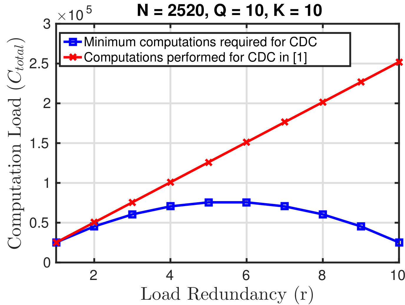 Figure 1
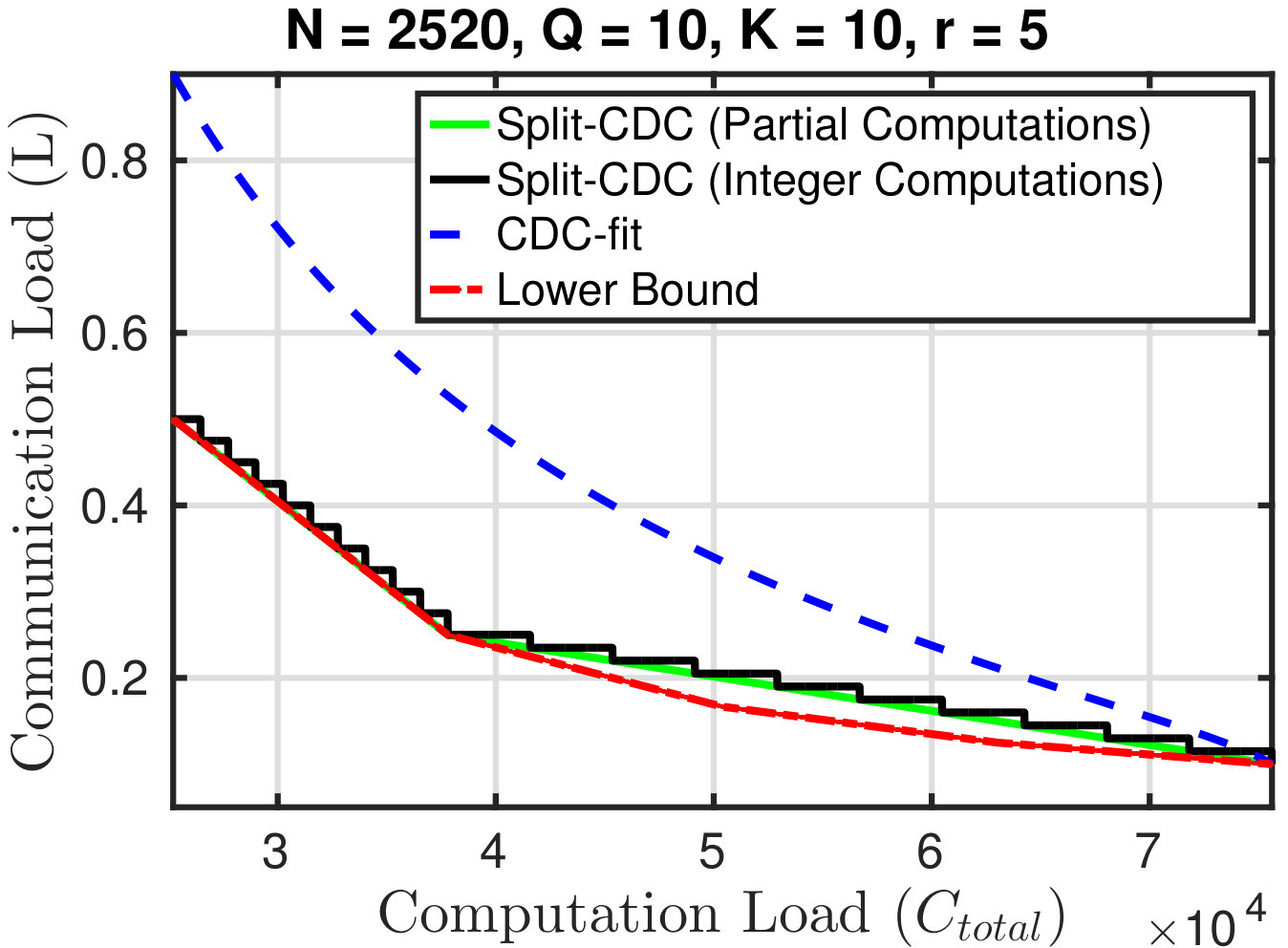 Figure 2
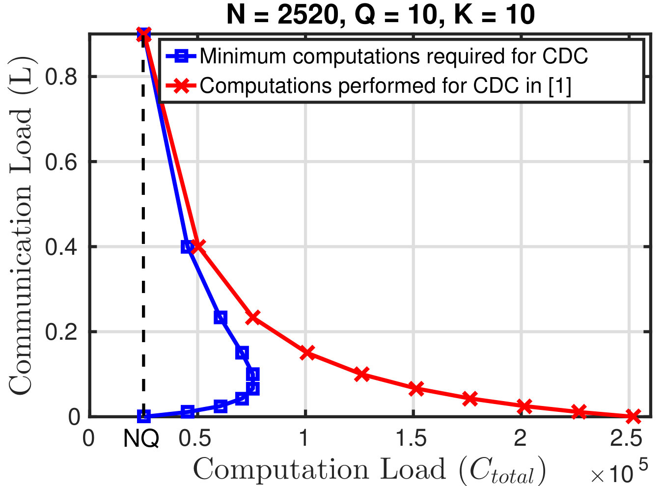 Figure 3
Peer Reviews
No public reviews on file for this paper yet. If you reviewed it on a platform where reviews are public (OpenReview, ICLR, NeurIPS, ICML), you can paste yours below so the community can read it here.
Videos
No videos yet. Explain this paper in a talk, walkthrough, or lecture? Add one.
Communication vs Distributed Computation:
an alternative trade-off curve
Yahya H. Ezzeldin, Mohammed Karmoose, Christina Fragouli University of California, Los Angeles, CA 90095, USA,
Email: {yahya.ezzeldin, mkarmoose, christina.fragouli}@ucla.edu
Abstract
In this paper, we revisit the communication vs. distributed computing trade-off, studied within the framework of MapReduce in [1]. An implicit assumption in the aforementioned work is that each server performs all possible computations on all the files stored in its memory. Our starting observation is that, if servers can compute only the intermediate values they need, then storage constraints do not directly imply computation constraints. We examine how this affects the communication-computation trade-off and suggest that the trade-off be studied with a predetermined storage constraint. We then proceed to examine the case where servers need to perform computationally intensive tasks, and may not have sufficient time to perform all computations required by the scheme in [1]. Given a threshold that limits the computational load, we derive a lower bound on the associated communication load, and propose a heuristic scheme that achieves in some cases the lower bound.
I Introduction
Distributed computation across a set of wireless networked servers is well motivated for several practical constraints: we may want to speed up computation time so as to finish a computation faster; we may have partial view of the files needed for computation across servers; we may have limited memory in each server; or we may be motivated by energy constraints. In this paper we consider the distributed computing framework studied in [1], that follows the architecture of MapReduce [2].
Our starting observation is that, the system in [1] does not explicitly separate computation from storage. The system uses a cluster of servers to compute output functions from input files. Each file is stored in different servers, balancing the amount of storage across servers. The work in [1] calculates the trade-off between the amount of computation and communication that servers need to do for such file placement. However, an underlying assumption of the derived trade-off, is that each server performs all possible computations on all the files stored in its memory. It is natural to ask: is it indeed useful to perform all possible computations?
The following simple example illustrates that this is not always the case. Consider a cluster with servers, files and output functions. All files are available at each server and each server is required to compute only one of the output functions. In this case, instead of performing computations per server (as assumed in [1]), each server only needs to perform computations related to its dedicated output function, i.e., only 3 computations are needed per server.
Our first contribution is to generalize this observation and derive an alternative trade-off curve to the scheme in [1]. We explicitly use three parameters: the total amount of computation required; that captures the memory requirements; and the communication load . We consider the placement and communication scheme in [1], and calculate the minimum number of computations each server needs to perform. We take into account the amount computed by the server for its assigned output functions, the amount that need to be communicated to other servers, and the amount needed to use as side information to decode transmissions from other servers.
We then proceed to examine the case where servers need to perform computationally intensive tasks, and in particular, do not have sufficient time to perform all computations the curve in [1] requires. Such a scenario may occur in wireless, where we may have cheap mobile devices with low computational power that need to cooperatively perform time-critical operations, for scientific computing or virtual reality applications. We ask, if the cluster is limited to perform an amount of computation below a threshold, what is the resulting minimum communication required to achieve the function computation.
Our second contribution is to derive a lower bound for the communication-computation trade-off when a cluster has a limited computation budget. For this lower bound, we assume that the files are distributed across the cluster with a predetermined level of redundancy that does not grow with the available computation budget. We show that a scheme directly inferred from [1] performs poorly when compared against the derived lower bound. Finally, we develop a distributed computing scheme inspired by [1] and show through numerical evaluation that the communication-computation trade-off it provides is comparable to the aforementioned lower bound.
Related Work. Minimizing communication load for distributed computation tasks has received considerable attention in the literature: starting from distributed boolean function computation between two parties [3, 4] to the more generalized theory of communication complexity [5, 6]. A key concept in reducing the needed amount of communication is through network coding. A prominent example of this concept is in the context of distributed cache networks [7, 8, 9], where coding is used in either the data placement or data delivery phases to reduce the amount of communication in the delivery phase. Recently, coding was also considered in the context of distributed computing systems that are based on the MapReduce framework [1, 10, 11]. In fact, the authors in [1] provided a Coded Distributed Computing (CDC) scheme which reduces the amount of communication needed in the data shuffling phase by using coded multicast transmissions. Our work differs in that we separate computation and storage, and thus derive alternative trade-off curves depending on the relative values of these parameters.
II System Model
Notation. Calligraphic letters denote sets through out the paper. denotes the cardinality of the set . The expression denotes the set of integers from to .
MapReduce framework. We consider a cluster of servers that computes output functions , , from input files , . In this paper, we assume that the servers share a lossless broadcast domain: a transmission from a server can be losslesly received by all other servers.
We assume the cluster uses a MapReduce framework to compute the set of functions in a distributed manner. MapReduce is based on the assumption that each output function can be calculated as a function of some intermediate processing of the files. In other words, , where is the intermediate value computed from file relevant to the output function , and has length bits. In MapReduce terminology, the intermediate value is computed (or “mapped”) using a map function and “reduces” the intermediate values to output .
Based on this decomposition, the computation model in [1] consists of three phases: Map, Shuffle and Reduce. Additionally, a Placement phase distributes files and tasks among the servers in the cluster. We next describe each of the phases:
-
Placement Phase: Each server is loaded with a subset of the files, such that . Each server is also assigned to compute a partition of the output functions, where .
-
Map Phase: Each server computes a subset of the intermediate values related to , i.e., . At the end of the Map phase, the assigned computation subsets satisfy that .
Remark 1**.**
In MapReduce, files are mapped by presenting them as pairs to a function that outputs a set of intermediate pairs based on the input pair. Although, the same build is used across the servers, the function can output different sets intermediate values based on the server ID by including this information in the .
-
Shuffle Phase: For a server to compute a function where , it needs all the intermediate messages . Thus in the Shuffle phase, the servers exchange intermediate values, such that each server has access to all its needed sets . The shuffling scheme can be described as follows: each server creates a message that is a function of its locally computed intermediate values and broadcasts this message to the remaining nodes.
-
Reduce Phase: In the Reduce phase, server uses its locally computed intermediate values and the received transmissions to decode the set of the needed intermediate values , . Using , the nodes can now compute the desired functions , .
Performance metrics. We measure the performance of this computation cluster across three parameters: the load redundancy (), the computation load () and the communication load (), defined as follows:
Load Redundancy. We define the load redundancy as the average number of times a file is assigned across the servers. We denote this by , i.e., . Load redundancy captures memory constraints.
Computation Load. We define the computation load as the total number of computations performed across servers in the cluster.
Communication Load. We define the communication load , as the number of bits transmitted in the Shuffle phase normalized by , where is the number of bits used to represent and is the total number of bits in all intermediate values , for and . From the definition, we have .
The definitions of and follow [1]; however in this paper, we explicitly separate the redundancy from the computation load, and use different parameters for each.
III On the relation between redundancy and computation
An underlying assumption in [1] is that each server must compute all the intermediate value for its stored files . In other words, . In this case, the load redundancy is linearly proportional to the total number of computations in the system as and can be therefore regarded as the computation load. However, if the server can selectively choose which intermediate values of to compute in the Map phase (as long as the communication load is the same), then the total number of computations is not necessarily linearly correlated with .
Consequently, an increase in does not necessarily result in an increase in the number of computations performed by the cluster. For example, assume that and each server is required to compute 1 output function (without loss of generality, ). Then, we have for both and . For , each file is available at only one server, thus each server needs to compute all intermediate values for all files stored in its memory. For , all files are available at each server. Thus, each server needs only to compute intermediate values related to its output function. In both cases, the optimal communication load is achieved [1, Theorem 1]. Note that for , if the servers computed all intermediate values for their files, there would be computations instead of .
Later in this section, we characterize the minimum computation load needed by the Coded Distributed Computing (CDC) scheme in [1] in order to achieve the optimal communication load in [1, Theorem 1] for . As we see later, taking this minimum computation load into account changes the trade-off in [1] for CDC. As a preliminary to that discussion, we next briefly describe the CDC scheme in [1].
An overview of the CDC scheme. Assume that and are sufficiently large so that and for some . The CDC scheme operates as follows (see [1] for a complete description):
-
Placement Phase: A disjoint subset of the files is assigned to each subset of servers where . Every server is thus assigned a set of files and every partition of these files is shared with a unique set of other servers. Every server is also assigned a unique subset of the output functions to calculate such that .
-
Map Phase: Every server computes all possible intermediate function values for the files it has.
-
Shuffling Phase: The shuffling phase repeats the following procedure for every set of size :
(i) For every , define and identify as
[TABLE]
The set represents the intermediate values that are needed by server to compute functions in , which can be computed exclusively by all servers in (recall that a file is replicated at exactly servers). Note that .
(ii) Split every intermediate value in into disjoint parts of bits and associate each part with a server in . Thus we split the set into partitions denoted by , , each of size . Each server will be responsible to convey its part to server with coded broadcast transmissions.
(iii) After splitting all sets for all (we have such sets), server sends the bit-wise XOR of all the -bit parts in , i.e., it makes broadcast transmissions each of size bits. Each transmission is useful to all other nodes in ; moreover, each server in has the required side information to decode the part it needs.
- Reduce Phase: In the reduce phase, every server uses its locally computed intermediate values and the decoded intermediate values in the shuffling phase to compute the output functions assigned to it in the initialization phase.
Next we discuss the minimum computation load needed for the CDC scheme.
Minimum Computations. The next proposition characterizes the minimum computation required by the CDC scheme.
Proposition 1**.**
For the placement scheme in [1] with , the communication load can be achieved with computation load
[TABLE]
Proof.
We first note that every server locally computes all intermediate values required by the functions in and corresponding to the files in ; we denote these intermediate values as . Thus, we have . Note that . In addition to , server also performs a set of computations required to carry out shuffling in the CDC scheme. We denote this set by . To calculate the number of computations in , we distinguish between computations required by server to decode its needed intermediate values (from transmissions in the shuffling phase) and the computations needed to create its transmissions in the shuffling phase.
Observe (from the description of the CDC scheme earlier and in [1]) that in any of size where , server uses the sets to construct its transmission. In addition, since the remaining parts will be XOR-ed (at the other servers) with parts needed by server , then server should compute the intermediate values in order to decode its requested intermediate values as well as construct its transmissions in the shuffling phase. This amounts to computations for every set . Thus, the total number of computations by server , , is
[TABLE]
where: (i) follows since server appears in only subsets of size ; (ii) and (iii) follow from the assumptions that and . From symmetry, the total number of computations in the Map phase equals . ∎
Note from (2) that is quadratic in . Thus, we cannot view as a direct measure of computation load since both the communication load as well as the number of computations reduce for . Fig. 3 shows the relation in (2) for and versus the number of computations if a server compute all map functions for each of its stored files. If we use [1, Theorem 1] and Proposition 1 to couple and , then we get the trade-off shown in Fig. 3 for the CDC scheme, where the red line is a scaled version of the trade-off in [1]. From Fig. 3, it can be seen that if we are free to choose for a given , then the optimal trade-off happens at ; by picking . This gives a communication load equal to zero while achieving the minimum computation load. This observation suggests that we can better understand the communication-computation trade-off, if we consider it with a predefined redundancy load () that does not change with the computation load .
Thus, in the remainder of the paper, we consider as a parameter of the cluster (with and ), and show how we can exploit this redundancy to perform coded distributed computing when at most computations are allowed.
IV An Achievable Communication-Computation Trade-off
Consider a distributed computing cluster with parameters and load redundancy , where represents the number of times each file is stored across the servers in the cluster. For our discussion in this section, we assume that and that the file placement (for a given ) follows the strategy in [1]. We are interested in answering the question: If the cluster is allowed to perform at most computations, what is the minimum communication load needed in order to compute output functions using the cluster ?
If , then from Proposition 1, we can directly use the CDC scheme described in [1], to achieve the optimal communication load . However, when , then the available computation budget is not enough to perform the shuffling and decoding required by the CDC scheme. In this case, can the CDC scheme be adapted to work with a restrictive computation budget? From [1], we can infer a simple modification to the CDC scheme, which we refer to as CDC-fit. In this scheme, we use CDC on the cluster while operating it with a lower load redundancy that fits the computation constraints. In other words, we pick and operate the cluster as if the files are only repeated times. This ensures that there are enough computations to satisfy CDC for and achieve the communication load . A natural question to ask here is whether this is the best possible approach?
To characterize this, we next develop a lower bound on the communication load when the cluster has a computation load and load redundancy .
Lower Bound on Communication load. We provide here a lower bound on the communication load for only a particular class of shuffling schemes. In this class, given a broadcast transmission sent during the shuffling phase, server can decode its required intermediate value from that transmission using only side information that it has locally computed. i.e., it does not rely on future transmissions to provide it with enough linear combinations to decode its required intermediate values. In what follows, an -type transmission denotes a broadcast transmission made by a server during shuffling, which consists of the XOR of equally-sized parts of intermediate values. The weight of an -type transmission is the size of the intermediate value parts used in the transmission.
In order to relax our lower bound, we assume that a server can perform partial computations on the files, i.e., if a server wants to transmit a fraction of bits (with ) of (recall is made of bits), then it only expends of a computation. With this assumption, we can observe the following properties of our cluster:
Obs. 1. Each server has files stored locally, and needs to receive intermediate values through shuffling.
Obs. 2. For a cluster with load redundancy , all feasible transmission have . This follows by noting that an -type transmission is assumed to satisfy servers 111If it is only useful for less than servers then the transmitter could have XOR-ed less intermediate values to generate the transmission.. Therefore, each intermediate value involved in this transmission is computed once at the transmitter, and computed once at each of the other servers which would utilize this intermediate value as side information to decode the transmission. Since each file is repeated across servers, then .
Obs. 3. In the shuffling phase, each -type transmission and weight incurs an added computation cost to the cluster equal to . To see this, note that the server sending this transmission makes computations. Moreover, an -type transmission serves servers, each of which would have to do computations to acquire the needed side information. Therefore we get .
Let be the number of -type transmissions. Then, the communication load for a shuffling scheme is lower bounded by the solution of the following Linear Program (LP)
[TABLE]
where: (i) the first constraint is a necessary condition for the shuffling phase to deliver intermediate values to each server in the cluster; (ii) the second condition is a necessary condition for the total computation (local computations and shuffling computations) to not exceed . Note that the result of the LP is a lower bound to the communication load since the first constraint is not sufficient to ensure that each server receives its needed intermediate values. Fig 3 compares the communication-computation trade-off for the aforementioned CDC-fit scheme with the lower bound in (4). The two trade-offs are close only towards high computation loads which allows the system to operate with an close to the natural of the cluster. Next, we propose a modification to the CDC scheme denoted as Split-CDC (S-CDC) that provide a communication-computation trade-off close to the trade-off suggested by the lower bound in (4).
Split-CDC (S-CDC). In order to introduce S-CDC, we make the following observations on the shuffling strategy in CDC.
Obs. 1. The set described in (1) is of size .
Obs. 2. For every subset of servers, the computations needed to satisfy all servers in is and the number of packets communicated among them is .
Obs. 3. From (1), it is not hard to see that for any subset such that , .
The previous observations suggest the following modification to the CDC scheme. Each subset of size can be split into disjoint subsets of smaller size. Each smaller subset can still be used to satisfy its members with the set as per Observation . Therefore, by using subsets of size different than , this would allow the scheme to exhibit different levels of communications and computations per (based on the size of the splits), as evident from Observation . The possible sizes of are , which we refer to as the split size. For , define and . Thus we can split set into disjoint sets of size and one set of size . For each set in , the needed number of computations is and the needed number of communicated packets is . If is not empty, then similar expression follow (except when , where we need computations and packets exchanges to send the intermediate values through unicast transmissions from any server in ). Finally, since , for every subset of size , CDC would naturally incur transmission rounds, each delivering exactly one intermediate value in for all servers in . Thus, our observations suggest that CDC can operate each of these transmission rounds with a different splitting size of ; thus the name Split-CDC (S-CDC). For a transmission round using split size , the total computations and communications per subset of size is
[TABLE]
S-CDC can now be formally described. Let be the fraction of the intermediate values in per subset that is delivered using split size . Then, S-CDC works as follows:
Determine the optimal values of for - this is done via solving the LP in (IV).
For each of size and split size :
- •
Split set into disjoint sets of size and one set of size .
- •
Use enough computations and communications per each of the subsets and as per the CDC scheme, to deliver intermediate values to all servers in . The computations and communications needed to do so is equal to and respectively.
What remains is to find the optimal values of . We do so via solving the following LP, which minimizes the total communication load subject to a total computation constraint.
[TABLE]
Note that in (IV), the variables are allowed to take non-integer values which means that we are allowing the servers to do partial computations of the intermediate values if that is what they will need to transmit or decode. To restrict partial computations, we can approximate the solution of (IV) to get a suboptimal integer-valued solution . Note that if an optimal solution of (IV) is non-integer, then there exists only two non-zero elements of ; we denote these two elements as and where . Then for our approximate solution, we define and . This gives us a communication load .
Fig. 3 compares the performance of S-CDC with the lower bound in (4) for and when partial computations are allowed. In this particular setup, Fig. 3 shows that by preventing partial computations, we only incur a small fraction of the communication load as an expense.
The reference list from the paper itself. Each links out to its DOI / PubMed record.
- 1[1] S. Li, M. A. Maddah-Ali, and A. S. Avestimehr, “Fundamental tradeoff between computation and communication in distributed computing,” in IEEE International Symposium on Information Theory (ISIT) , 2016, pp. 1814–1818.
- 2[2] J. Dean and S. Ghemawat, “Mapreduce: simplified data processing on large clusters,” Communications of the ACM , vol. 51, no. 1, pp. 107–113, 2008.
- 3[3] A. C.-C. Yao, “Some complexity questions related to distributive computing (preliminary report),” in Proceedings of the eleventh annual ACM symposium on Theory of computing , 1979, pp. 209–213.
- 4[4] A. Orlitsky and J. Roche, “Coding for computing,” IEEE Trans. on Information Theory , vol. 47, no. 3, pp. 903–917, 2001.
- 5[5] E. Kushilevitz and N. Nisan, “Communication complexity,” 2006.
- 6[6] K. Becker and U. Wille, “Communication complexity of group key distribution,” in Proceedings of the 5th ACM conference on Computer and communications security , 1998, pp. 1–6.
- 7[7] M. A. Maddah-Ali and U. Niesen, “Fundamental limits of caching,” IEEE Trans. on Information Theory , vol. 60, no. 5, pp. 2856–2867, 2014.
- 8[8] N. Karamchandani, U. Niesen, M. A. Maddah-Ali, and S. N. Diggavi, “Hierarchical coded caching,” IEEE Trans. on Information Theory , vol. 62, no. 6, pp. 3212–3229, 2016.