Tree-level vacuum stability of two-Higgs-doublet models and new constraints on the scalar potential
Xun-Jie Xu

TL;DR
This paper investigates the conditions under which the vacuum in two-Higgs-doublet models is stable at tree-level, providing new constraints on the scalar potential that are relevant for phenomenological analyses.
Contribution
It derives conditions ensuring the considered vacuum is the global minimum in 2HDMs, adding new theoretical constraints to stabilize the scalar potential.
Findings
Derived tree-level vacuum stability conditions for 2HDMs
Identified new constraints on the scalar potential parameters
Applied constraints to a specific 2HDM model
Abstract
The scalar potential of the two-Higgs-doublet model (2HDM) may have more than one local minimum and the usually considered vacuum could be located at one of them that could decay to another. This paper studies the condition that the usually considered vacuum is the global minimum which, combined with the bounded-from-below condition, will stabilize the vacuum at tree-level. We further apply these conditions to a specific 2HDM and obtain new constraints which could be important in phenomenological studies.
Click any figure to enlarge with its caption.
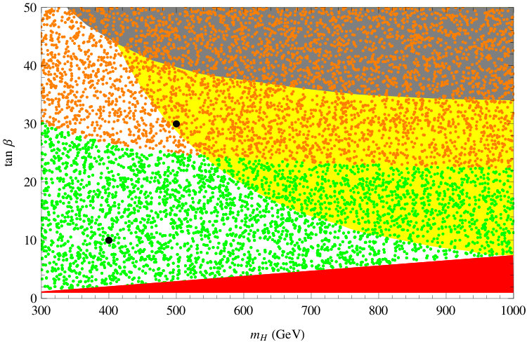 Figure 1
Peer Reviews
No public reviews on file for this paper yet. If you reviewed it on a platform where reviews are public (OpenReview, ICLR, NeurIPS, ICML), you can paste yours below so the community can read it here.
Videos
No videos yet. Explain this paper in a talk, walkthrough, or lecture? Add one.
Tree-level vacuum stability of two-Higgs-doublet models and new
constraints on the scalar potential
Xun-Jie Xu
Max-Planck-Institut für Kernphysik, Postfach 103980, D-69029 Heidelberg, Germany.
(March 18, 2024)
Abstract
The scalar potential of the two-Higgs-doublet model (2HDM) may have more than one local minimum and the usually considered vacuum could be located at one of them that could decay to another. This paper studies the condition that the usually considered vacuum is the global minimum which, combined with the bounded-from-below condition, will stabilize the vacuum at tree level. We further apply these conditions to a specific 2HDM and obtain new constraints which could be important in phenomenological studies.
I Introduction
As a simple extension of the Standard Model (SM), the Two-Higgs-Doublet Model (2HDM) is well motivated in many aspects, including supersymmetry Djouadi (2008), violation Lee (1973), axion models Kim (1987), etc. Besides, it also provides a very rich phenomenology in collider experiments Haber and Stal (2015); Chakrabarty and Mukhopadhyaya (2017); Capdequi Peyranere et al. (1991); Haber (2012); Ferreira et al. (2013a, 2014a, 2014b); Broggio et al. (2014); Bernon et al. (2015, 2016); Ferreira and Jones (2009); Ferreira et al. (2012a, b); Barroso et al. (2013a); Ferreira et al. (2013b, 2014c, 2014d); Dumont et al. (2014); Bhupal Dev and Pilaftsis (2014); Campos et al. (2017). Therefore the 2HDM, as well as many variations, have been extensively studied in recent years (see, e.g., Branco et al. (2012) for a comprehensive review).
In the 2HDM, an additional Higgs doublet is introduced to the scalar sector of the SM. The scalar potential contains not only self-coupling terms of each Higgs doublet but also several mixing terms of the two doublets. As a consequence, the potential may contain several different minima at which the scalar fields may obtain very different vacuum expectation values (VEVs). Depending on the configuration of the potential, it is possible that one of the doublets does not acquire a VEV (which appears in inert 2HDMs—see, e.g. Ma (2006a, b); Barbieri et al. (2006); Majumdar and Ghosal (2008); Lopez Honorez et al. (2007); Sahu and Sarkar (2007); Martinez et al. (2011); Melfo et al. (2011); Khan and Rakshit (2015)), or the VEVs break the symmetry Dubinin and Semenov (2003); Gunion and Haber (2005); Maniatis et al. (2008); Bian and Chen (2016); Grzadkowski et al. (2016), or even break the electromagnetic symmetry which should be avoided in model building. In many phenomenological studies on 2HDMs, the desired vacuum is usually imposed without checking whether the potential necessarily results in such vacuum. It has been discussed in Ferreira et al. (2004); Barroso et al. (2006a, b, c); Ivanov (2007a); Barroso et al. (2006d); Ivanov (2008); Barroso et al. (2007); Ivanov (2007b, 2009); Ivanov and Nishi (2010); Barros e Sa et al. (2008); Ginzburg et al. (2010); Ivanov (2010); Battye et al. (2011); Barroso et al. (2013b, c, d, e); Ivanov and Silva (2015), however, that more than one local minimum could coexist in the 2HDM potential, which implies the desired vacuum111In this paper we refer to the vacuum that is compatible with all experimental observations as the desired vacuum. might be only a local minimum that could decay into a deeper one by quantum tunneling Coleman (1977); Callan and Coleman (1977). If this could happen, the vacuum would be unstable.
To avoid vacuum instability we expect a global minimum222In principle, if the vacuum is a local minimum but the decay rate is low enough, then it can be metastable and the model is still valid. We will discuss this issue in Sec. IV. for the desired vacuum, which requires some new constraints on the potential parameters, in addition to the bounded-from-below (BFB) constraints Klimenko (1985); Maniatis et al. (2006); Ivanov (2007a); Ferreira and Jones (2009). Although it has been noticed in the literature Ferreira et al. (2004); Barroso et al. (2006a, b, c); Ivanov (2007a); Barroso et al. (2006d); Ivanov (2008); Barroso et al. (2007); Ivanov (2007b, 2009); Ivanov and Nishi (2010); Barros e Sa et al. (2008); Ginzburg et al. (2010); Ivanov (2010); Battye et al. (2011); Barroso et al. (2013b, c, d, e); Ivanov and Silva (2015) that the vacuum could be unstable due to localness of the minimum, in most phenomenological studies only the BFB constraint is taken into account for the vacuum stability.333 In addition to the BFB constraint, the unitarity bound Casalbuoni et al. (1986, 1988); Maalampi et al. (1991); Kanemura et al. (1993); Arhrib (2000); Akeroyd et al. (2000); Ginzburg and Ivanov (2003, 2005); Horejsi and Kladiva (2006) is another theoretical constraint on the potential which has been taken into account in many phenomenological studies. Actually in the Higgs triplet model [the SM extended by an triplet Higgs], recently we have derived explicit expressions of the conditions to keep the desired vacuum globally minimal Xu (2016). It turns out that such conditions lead to interesting constraints on the masses of the scalar bosons in the Higgs triplet model. Therefore, we expect that in 2HDMs this issue may also have phenomenologically interesting consequences and should be taken into consideration in future studies on 2HDMs.
In this paper, we will investigate the 2HDM potential and derive the condition for a selected minimum being the global one in order to stabilize the corresponding vacuum. The method is similar to Xu (2016), in which we first analytically compute all possible local minima and then compare them with each other. We will adopt the most general potential including all renormalizable terms that respect the gauge symmetries of the SM. In some specific models, e.g. the type I and type II 2HDMs with symmetries444The type I 2HDM couples all quarks to one Higgs doublet (denoting the other as ), which can be realized by the symmetry: , . The type II 2HDM couples down-type right-handed quarks and up-type right-handed quarks to and respectively, which can be realized by assigning the charge to and . In both cases, terms in the scalar potential containing odd numbers of should be absent. to avoid tree-level flavour-changing neutral currents (FCNC), some terms in the potential are absent. They can be regarded as special cases of the most general potential we adopted so our calculations also apply to these special cases. Based on the analytical calculations, a numerical process is established to determine whether a selected minimum is globally minimal. Applying this process to a specific -conserving type I 2HDM with softly broken symmetry Haber and Stal (2015), we show that the parameter space of the scalar potential can be considerably constrained by the vacuum stability and in a certain scenario the constraint is even stronger than the LHC constraint.
The issue that the 2HDM vacuum could be unstable if it was not the global minimum has been studied in the literature for more than a decade Ferreira et al. (2004); Barroso et al. (2006a, b, c); Ivanov (2007a); Barroso et al. (2006d); Ivanov (2008); Barroso et al. (2007); Ivanov (2007b, 2009); Ivanov and Nishi (2010); Barros e Sa et al. (2008); Ginzburg et al. (2010); Ivanov (2010); Battye et al. (2011); Barroso et al. (2013b, c, d, e); Ivanov and Silva (2015). In an early work Ferreira et al. (2004) it has been shown that, for a potential without explicit breaking, if a minimum preserving the electromagnetic and symmetries exists, then it is the global one. However it was also pointed out in Barroso et al. (2006b, 2007) that two neutral minima may coexist and have different potential depths. References Ivanov (2007a, 2008) adopt a geometric approach by reformulating the 2HDM potential in terms of 3-quadrics in the Minkowski space and prove that the potential can have at most two local minima. Furthermore, if the two local minima coexist and there is a discrete symmetry in the potential, then the two minima will both break or both preserve the symmetry. In a recent study Ivanov and Silva (2015) the criteria to guarantee that the desired minimum is global have been proposed. The method involves calculating a determinant and in some cases solving eigenvalues of a matrix numerically, which is different from the method we adopt in this paper.
The reminder of this paper is organized as follows. In Sec. II we analyze the most general scalar potential in 2HDMs and analytically compute all possible types of local minima. Then we discuss how to determine the global minimum in Sec. III with a numerical example to illustrate the method. In Sec. IV we study the vacuum stability with both the BFB condition and the requirement of a global minimum taken into account, focusing on the type I 2HDM with softly broken symmetry. Finally, we summarize at Sec. V. Some numerical examples which can be used to verify our calculations are described in detail in Appendix A.
II The scalar potential and local minima
With two Higgs doublets and (both have the same hypercharge ), the most general renormalizable scalar potential can be written as Wu and Wolfenstein (1994)
[TABLE]
There are three quadratic terms and seven quartic terms in Eq. (1), with four complex coefficients (, ) and six real coefficients (, , ), i.e., 14 real parameters in total. However due to the unitary basis transformation where is an matrix, three unphysical degrees of freedom can be removed so actually there are only 11 physical degrees of freedom Branco et al. (2012). In some 2HDMs due to additional symmetries [e.g. , , , etc.], some terms are absent. To apply the calculations below to these specific models, one only needs to set the corresponding couplings to zero. There are 8 degrees of freedom in the two doublets and . After spontaneous symmetry breaking, three of them become Goldstone bosons and the remaining five form massive scalar particles, including two -even scalar bosons (, ), one -odd scalar boson () and one charged scalar boson ().
An important feature of the above potential is that it is a quadratic functions of three invariants of the fields Botella and Silva (1995)
[TABLE]
where are real, non-negative and is complex. Since and are not invariant under transformations, we will use instead of in the following analysis. The potential expressed in terms of and is:
[TABLE]
Without boundary conditions, one can immediately find a minimum (to distinguish it from other minima, we will refer to it as the type A minimum) by solving
[TABLE]
Equation. (4) is a combination of linear equations with respect to , with the following explicit form:
[TABLE]
The solution of the above linear equation is given by Ferreira et al. (2004); Maniatis et al. (2006); Ivanov (2007a); Nishi (2007)
[TABLE]
where555Note that in many models due to some symmetries in the potential, the matrix could be noninvertible. For example, if are real and then does not exist. However, one can still use Eqs. (6) and (7) in this case by taking . In Sec. III we will present an example in this case.
[TABLE]
The potential value at this minimum is
[TABLE]
However, we should note that the three variables are subjected to some boundary conditions. From the definitions of and we have two boundary conditions
[TABLE]
Besides, since is a scalar product of two complex vectors, its absolute value should be less than or equal to the product of their lengths, which is . So we have
[TABLE]
The type A minimum exists only if the point computed via Eq. (6) is located in the region restricted by the above conditions.
Apart from the type A minimum, other minima could exist but they should be on the boundaries (9), (10) or (11) otherwise they would be determined by the off-boundary minimization equation (4) which has a unique solution, i.e. the type A minimum. There are four types of on-boundary minima, which depending on the boundaries will be referred to as the type B, C, D and E minima:
[TABLE]
Type B and C minima can be computed by setting or to zero and minimizing the potential with respect to or . This gives
[TABLE]
The corresponding potential values at these minima are given by
[TABLE]
[TABLE]
Type E is the simplest case. All fields and the potential value are zero at this minimum.
The remaining case, type D, is actually the desired vacuum in many 2HDMs with non-vanishing and , because implies the two complex vectors and are parallel to each other at the minimum, i.e. . Since the absolute value of is fixed by , the potential can be treated as a function of , and
[TABLE]
From we get
[TABLE]
where we have defined
[TABLE]
[TABLE]
[TABLE]
[TABLE]
The above calculation is basis independent. However, to represent it in a more conventional form, we may choose an appropriate basis so that
[TABLE]
which implies that the type D minimum corresponds to the vacuum usually adopted in many 2HDMs. In this basis, one can interpret as the well-known ratio
[TABLE]
and relate the value of at the minimum to the electroweak vacuum expectation value
[TABLE]
One can solve Eqs. (21), (22), and (23) with respect to (or ), , and to get the type D minimum of the potential, at least numerically. Since they are nonlinear equations, the solutions may be not unique. In general, all solutions should be taken into account, which makes the type D minima a little more complicated than the other types. We will show an example which has more than one type D minimum in Sec. III.
Finally, let us summarize all possible local minima of the scalar potential, as listed in Tab. 1. There are five types of minima, classified according to whether they locate on some boundaries [cf. Eqs. (9), (10), and (11)] in the space. Type A is not on any of the boundaries, which implies it has the most degrees of freedom in the minimization, while type E is actually on all the boundaries so it is completely fixed by these boundaries. To provide a straightforward understanding of them, the second row of Tab. 1 shows the zero components of and , where we use “” and “” to represent nonzero and arbitrary (zero or nonzero) values, respectively. However, one should be careful about the basis dependence. For any minimum of the potential, the transformation
[TABLE]
where is a unitary matrix would transform the vacuum to another equivalent vacuum, while the appearance of zero components in and is not invariant under this transformation. Therefore, and in Tab. 1 for each type of minima should be understood as a category of VEVs that can be transformed to such a form. For instance, if the potential is found to has a minimum at
[TABLE]
or
[TABLE]
then this minimum should be of type A (generally), since the doublets can be transformed to the form and . However, if it happens coincidentally that in Eq. (32), then this falls into type D, since the transformation will simultaneously set the upper components of and to zero.
To avoid the basis dependence, we recommend using instead of explicit forms of and . Once a minimum is found, one can compute the values of to see whether the minimum is located on some of the boundaries of Eqs. (9), (10) , and (11), which is the original definition of the five types of minima.
For any given potential in 2HDMs, one can exhaustively find all the possible minima by computing according to the third row of Tab. 1. But the corresponding minima do not necessarily exist, e.g. or computed in this way may be negative. So in Tab. 1 we also provide the conditions of existence of these minima, which should be checked after is computed. The existence conditions listed here are only necessary conditions, not sufficient, which implies the locations could be saddle points or even local maxima. But in the framework of this paper, this does not concern us because by comparing the potential values at these points we will take the lowest point among these candidates as the vacuum of the model, which must be the global minimum, provided that the potential is BFB.
III Global minima
As we have derived, there can be several types of minima in the scalar potential so it is possible that the desired vacuum is not located at a global minimum. This problem in 2HDMs has been studied in Refs. Ferreira et al. (2004); Barroso et al. (2006b, 2007); Ivanov (2008) where one can find some useful conclusions. First, it has been proved that at most two physically inequivalent local minima can coexist in the potential. This implies that among the five possible types of local minima, only one or two of them can actually exist in a certain potential while the others should be saddle points or local maxima. Second, the two minima (if exist) violate or conserve a discrete symmetry (if exist in the potential) simultaneously, e.g., -conserving and -violating minima cannot coexist in a -conserving potential.
Despite these conclusions, given a general 2HDM potential and a minimum of the potential, one still cannot determine the globalness of the minimum in a simple way. However, since we know how to find all possible local minima in the potential, there is a numerical process that enables us to determine whether a minimum is global or local.
For a given potential and one of its minima, denoting the location of this minimum as and the corresponding potential value as , if then obviously is not a global minimum because the potential value is larger than the type E minimum. If , then one proceeds as follows:
Compute for the minima of types A, B, and C listed in Tab. 1. 2. 2.
Check the existence condition for each of them. If it is violated then it will not be considered anymore. 3. 3.
Compute the potential values at the remaining minima; if any of them are lower than then is not a global minimum. 4. 4.
Otherwise, numerically solve Eqs. (21), (22) and (23) and compare with the potential values of these solutions. If is still the lowest, then is the global minimum.
Here, in principle, we can also include type D in step 1 and remove step 4. However, type D involves solving non-linear equations numerically, which consumes much more CPU usage for computers to work it out than types A, B and C. According to our numerical experience, if is not a global minimum, in many cases it can be excluded by comparing with the first three types of minima. Therefore we leave the calculation of type D minima as the last step, which optimizes the program considerably.
The above process is simple to be realized in programming so it can be readily included in numerical analyses of 2HDMs. Actually, the situation is similar to the BFB condition. Despite that there have been some analytical expressions of the BFB condition in some special cases such as Branco et al. (2012), for the most general potential there has not been a simple criterion for BFB. Currently a numerical process that combines necessary analytical results is able to achieve this, which has been adopted in the program 2HDMC Eriksson et al. (2010). Likewise, one may also adopt the similar numerical process proposed above to check whether a minimum is global.
To illustrate the above process, we will analyze a specific example, which also serves as a benchmark to show that requiring the vacuum to be globally minimal provides new constraints on the model. In a specific scenario of 2HDM studied in Haber and Stal (2015), the potential parameters take the following values:888Corresponding to GeV, GeV, , , , and in the hybrid basis Haber and Stal (2015), which are taken as an input in the code 2HDMC Eriksson et al. (2010) to generate the parameters in Eqs. (34) and (35).
[TABLE]
[TABLE]
This example is well compatible with recent constraints from LHC Dumont et al. (2014); Haber and Stal (2015), including both the observed Higgs signal and non-observation of additional Higgs states. The vacuum of this model is at GeV and , corresponding to a minimum at
[TABLE]
The potential value at this minimum is .
Now we would like to know whether this minimum is global or local. Since , we neglect the type E minimum. Computing for type A, B and C minima gives999In this example we have which makes non-invertible. Such cases appear occasionally in 2HDM potentials with some symmetries. To validate Eqs. (6) and (7), one can simply add a small perturbation to and compute .
[TABLE]
However, the solution of type A violates its existence condition since . Thus we only need to compute the potential values at type B and C minima:
[TABLE]
As we can see, so we can conclude that is not the global minimum without solving the nonlinear equations of type D.
Nevertheless, if we further solve the equations of type D, we will know the actual vacuum structure. According to the results in Appendix A, there are four solutions of type D in this example, denoted as D1, D2, D3 and D4, with the following potential values:
[TABLE]
These values imply that the global minimum of this potential is D1 while is actually identical to D2 which is a local minimum101010In general, one needs to compute the second-order derivatives (Hessian matrix) to make sure that it is not a saddle point or a local maximum. However, this is not necessary for since we know the mass spectrum of the scalar bosons (see Appendix A) is above zero, which implies the eigenvalues of the Hessian matrix are all positive.. Since there can be at most two physically inequivalent minima in a 2HDM potential, we immediately know that these two minima must be D1 and D2. As a consequence, the other local minimum candidates such as and in Eq. (38) can only be saddle points or local maxima, despite that is lower than the local minimum .
IV Tree-level vacuum stability and its constraints
on 2HDMs
In the previous section, we have seen an example of the 2HDM potential in which the desired vacuum is not a global minimum, though it is compatible with all constraints from LHC. In such case, the vacuum may decay into a deeper minimum via quantum tunneling which makes the vacuum unstable. This situation should be avoided in any valid 2HDM. Consequently we will have a new constraint on the model by requiring that the desired vacuum is a global minimum.
We would like to comment here that this is not completely equivalent to the vacuum stability. First, if the decay rate is low enough, the vacuum can be metastable which means the lifetime of the vacuum is longer than the age of the universe so that the metastable vacuum still survives today. Second, even if the vacuum at tree level is absolutely stable, in the effective potential including loop corrections Staub (2017); Dorsch et al. (2017) the vacuum could be unstable. A well-known example is the SM in which the potential would be negative around GeV due to large loop corrections from the top quark Lindner et al. (1989). An elaborate investigation Buttazzo et al. (2013) suggests that with current best-fit values of top quark and Higgs masses the SM vacuum is metastable.
In principle, one may take the metastability and loop corrections into consideration in 2HDMs as well. However, both of them are only important when the parameters of the model are near some critical configurations (e.g. the SM metastability depends critically on the top quark mass). In 2HDMs many parameters are still far from being precisely determined while in contrast, the potential parameters of the SM have been known precisely from the Higgs mass and the Fermi constant. Therefore at the current stage, we should not be concerned with these two issues. Instead, we only consider the absolute stability of vacuum at tree level.
Next we will focus on a specific 2HDM to study the constraint from the vacuum stability on some physical quantities. In a -conserving 2HDM with a softly broken symmetry that has been studied in Ref. Haber and Stal (2015), the quartic terms are invariant under the transformation
[TABLE]
which leads to
[TABLE]
The quadratic term , however, softly breaks the symmetry. All quartic and quadratic coefficients in the potential are real due to the symmetry. After spontaneous symmetry breaking, the two Higgs doublets are expected to acquire -conserving VEVs:
[TABLE]
Apart from three Goldstone bosons, there are four mass eigenstates of the scalar fields, including two -even Higgs fields and , a -odd field and a charged Higgs . Their masses are given by Gunion and Haber (2003)
[TABLE]
[TABLE]
[TABLE]
where the matrix is defined as
[TABLE]
Diagonalizing the matrix gives the eigenvalues and the mixing angle (-\pi/2$$\leq\alpha\leq$$\pi/2) between the two eigenstates,
[TABLE]
In Ref. Haber and Stal (2015), a “hybrid” basis is adopted in specifying the input parameters of the model. The input parameters in the hybrid basis are where and are defined as
[TABLE]
[TABLE]
[TABLE]
This basis has already been included in the code 2HDMC Eriksson et al. (2010) which facilitates the input of valid model parameters. Hence we will use 2HDMC in scanning the parameter space. We focus on a specific scenario with the major portion of its parameter space still compatible with the recent LHC constraints. In the hybrid basis, the input parameters are
[TABLE]
and
[TABLE]
To show the constraint from the vacuum stability, we randomly generate samples with the input parameters given in Eqs. (50) and (51). We use 2HDMC to compute the corresponding potential parameters and and also to check the BFB condition of the potentials. For those samples with BFB potentials, we proceed to check whether the electroweak vacuum is a global minimum, with the method introduced in Sec. III. For simplicity, we call it the GM (global minimum) condition. The result is presented in Fig. 1, where the red region is excluded by the BFB bound, the orange points violate the GM conditions and the green points satisfy both the BFB and the GM conditions. Two examples (one of them has been studied in Sec. III) are marked in Fig. 1 by black points, with the numerical details given in Appendix A, which can be used to check the calculations. The gray region represents the constraint from direct searches from LHC, taken from Haber and Stal (2015). The yellow region violates the unitarity bound Casalbuoni et al. (1986, 1988); Maalampi et al. (1991); Kanemura et al. (1993); Arhrib (2000); Akeroyd et al. (2000); Ginzburg and Ivanov (2003, 2005); Horejsi and Kladiva (2006), checked by 2HDMC. As is shown in the plot, there is a considerably large part of the parameter space that can be excluded by the stability of the electroweak vacuum at tree level. In the specific scenario considered here, the GM constraint is even stronger than the LHC constraint and complementary to the unitarity bound. One should note that this is based on the type I -conserving 2HDM studied in Ref. Haber and Stal (2015) in a particular scenario, which should not be regarded as a general conclusion. Nevertheless, the result presented in Fig. 1 suggests that the vacuum stability at tree level should be taken into account in theoretical constraints on 2HDMs.
V Conclusion
In the most general scalar potential of 2HDMs, more than one minimum may coexist while the usually considered vacuum could be located at a local minimum that could decay into a deeper one. We have seen such an example in Sec. III. To avoid vacuum instability at tree level, we require a global minimum for the vacuum. Therefore in this paper we study on the local and global minima of the 2HDM potential and try to find out the condition of a selected minimum being globally minimal.
According to our analytical calculations, there are five different possible types (denoted as type A to E) of minima, which are all summarized in Tab. 1. Regarding the question of which is the global minimum, though there has not been a simple answer, a numerical process is proposed to address it, which is practically applicable in phenomenological studies.
The requirement of a global minimum will generate a new constraint on the model. In a -conserving 2HDM with softly broken symmetry, we have shown in Fig. 1 that such a new constraint can be considerably significant in reducing the allowed parameter space. In general, this constraint can be applied to many other 2HDMs, which will be studied in future work.
Acknowledgements.
XJX would like to thank Carlos Yaguna for some useful discussions at the early stage of this work, and Werner Rodejohann and Florian Goertz for carefully reading the manuscript and many helpful suggestions.
Appendix A Numerical examples
In this appendix we show two examples with numerical information in detail. One example violates the GM condition which will be called example (1) below. The other satisfying the GM condition is called example (2). Both are displayed in Fig. 1.
The input parameters in the hybrid basis are [here and henceforth we add superscripts (1) and (2) on the corresponding quantities to distinguish between them]
[TABLE]
[TABLE]
The output potentials computed by 2HDMC are
[TABLE]
[TABLE]
[TABLE]
[TABLE]
The masses of scalar bosons computed according to Eqs. (43), (44), and (45) are
[TABLE]
[TABLE]
The mixing angle from Eq. (46) is
[TABLE]
The first three types of minima computed according to Tab. 1 are
[TABLE]
[TABLE]
[TABLE]
[TABLE]
and
[TABLE]
[TABLE]
[TABLE]
[TABLE]
The type D minima are obtained by numerically solving the non-linear equations (21), (22) and (23). There are four different solutions in example (1) which are denoted as D1, D2, D3 and D4:
[TABLE]
[TABLE]
[TABLE]
[TABLE]
The corresponding potential values are
[TABLE]
So D1 is the global minimum.
As for example (2), there is only one solution at
[TABLE]
and the potential value is
[TABLE]
which is the global minimum of the potential in example (2).
The reference list from the paper itself. Each links out to its DOI / PubMed record.
- 1Djouadi (2008) A. Djouadi, Phys. Rept. 459 , 1 (2008) , ar Xiv:hep-ph/0503173 [hep-ph] . · doi ↗
- 2Lee (1973) T. D. Lee, Phys. Rev. D 8 , 1226 (1973) , [,516(1973)]. · doi ↗
- 3Kim (1987) J. E. Kim, Phys. Rept. 150 , 1 (1987) . · doi ↗
- 4Haber and Stal (2015) H. E. Haber and O. Stal, Eur. Phys. J. C 75 , 491 (2015) , [Erratum: Eur. Phys. J.C 76,no.6,312(2016)], ar Xiv:1507.04281 [hep-ph] . · doi ↗
- 5Chakrabarty and Mukhopadhyaya (2017) N. Chakrabarty and B. Mukhopadhyaya, (2017), ar Xiv:1702.08268 [hep-ph] .
- 6Capdequi Peyranere et al. (1991) M. Capdequi Peyranere, H. E. Haber, and P. Irulegui, Phys. Rev. D 44 , 191 (1991) . · doi ↗
- 7Haber (2012) H. E. Haber, in International Workshop on Future Linear Colliders (LCWS 11) Granada, Spain, September 26-30, 2011 (2012) ar Xiv:1203.2631 [hep-ph] .
- 8Ferreira et al. (2013 a) P. M. Ferreira, R. Santos, H. E. Haber, and J. P. Silva, Phys. Rev. D 87 , 055009 (2013 a) , ar Xiv:1211.3131 [hep-ph] . · doi ↗