A Geometric Approach to Dynamical Model-Order Reduction
Florian Feppon, Pierre F.J. Lermusiaux

TL;DR
This paper introduces a geometric framework for model-order reduction of stochastic PDEs, analyzing the manifold of fixed rank matrices and deriving dynamical systems that optimize low-rank approximations.
Contribution
It provides a detailed geometric analysis of the fixed rank matrix manifold and develops explicit dynamical systems for low-rank approximation and model reduction.
Findings
The curvature of the fixed rank matrix manifold is characterized.
Error bounds for the DO approximation are established based on singular value gaps.
Algorithms for adaptive low-rank matrix approximation are proposed.
Abstract
Any model order reduced dynamical system that evolves a modal decomposition to approximate the discretized solution of a stochastic PDE can be related to a vector field tangent to the manifold of fixed rank matrices. The Dynamically Orthogonal (DO) approximation is the canonical reduced order model for which the corresponding vector field is the orthogonal projection of the original system dynamics onto the tangent spaces of this manifold. The embedded geometry of the fixed rank matrix manifold is thoroughly analyzed. The curvature of the manifold is characterized and related to the smallest singular value through the study of the Weingarten map. Differentiability results for the orthogonal projection onto embedded manifolds are reviewed and used to derive an explicit dynamical system for tracking the truncated Singular Value Decomposition (SVD) of a time-dependent matrix. It is…
Click any figure to enlarge with its caption.
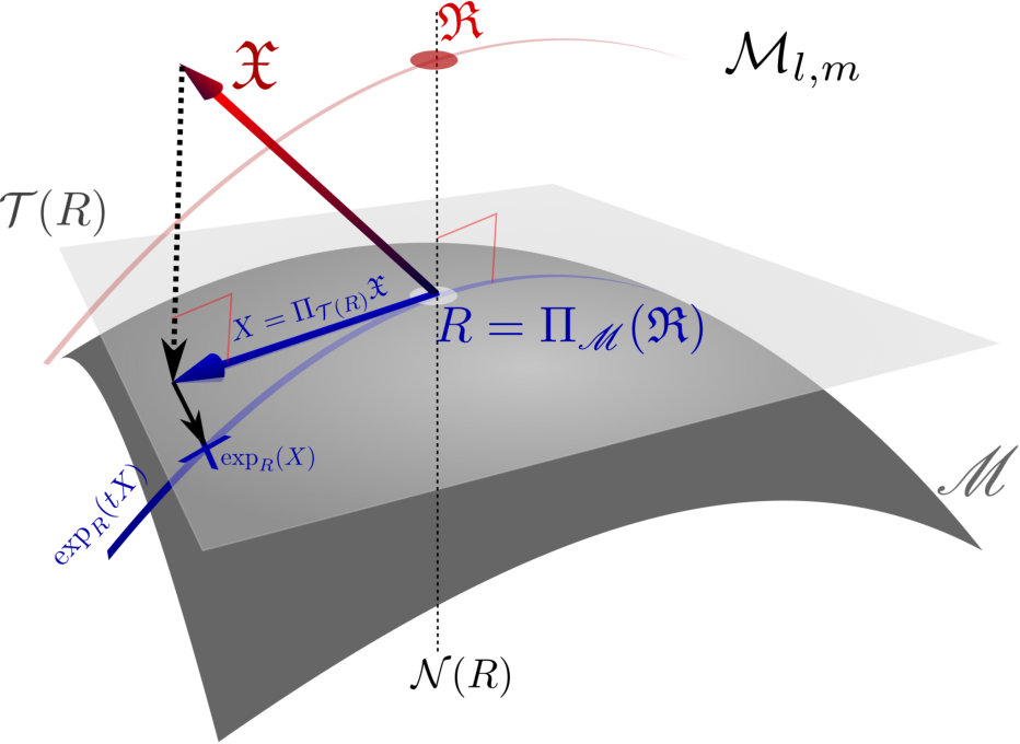 Figure 1
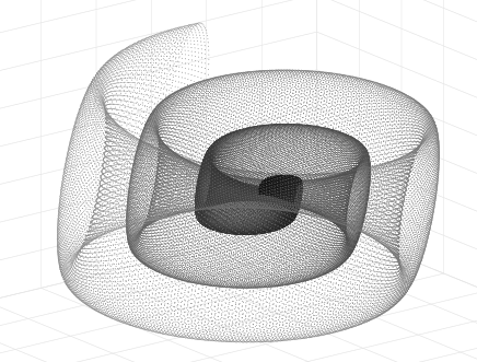 Figure 2
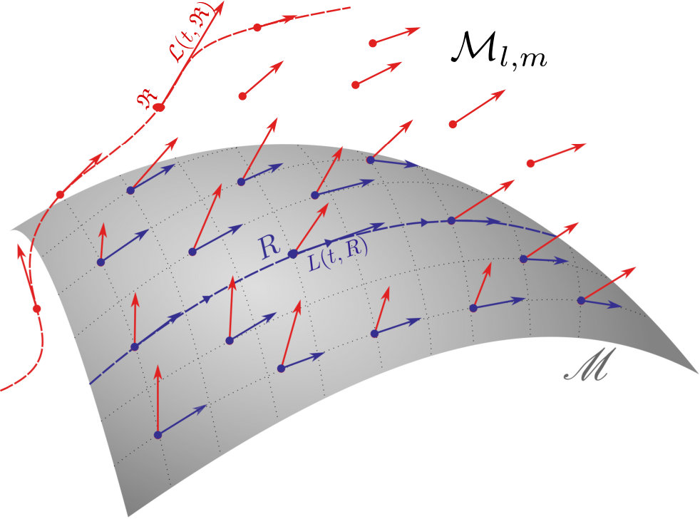 Figure 3
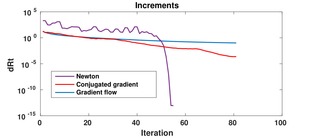 Figure 4
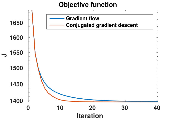 Figure 5
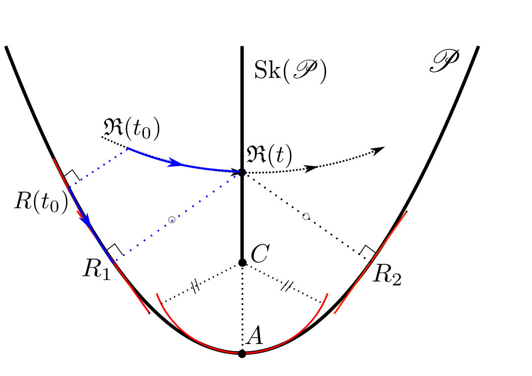 Figure 6
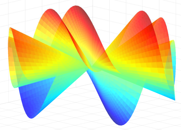 Figure 7
| Space of -by- real matrices | |
| Space of -by- matrices that have full rank | |
| Rank of a matrix | |
| Fixed rank matrix manifold | |
| Group of -by- orthogonal matrices | |
| Stiefel Manifold | |
| Point with and | |
| Tangent space at | |
| Tangent vector at | |
| Horizontal space at | |
| with | |
| and | |
| Orthogonal projection onto the plane | |
| Skeleton of | |
| Orthogonal projection onto (defined on ) | |
| Identity mapping | |
| Transpose of a square matrix | |
| Frobenius matrix scalar product | |
| Frobenius norm | |
| Non zeros singular values of | |
| Time derivative of a trajectory | |
| Differential of a function in direction | |
| Differential of the projection operator applied to |
Peer Reviews
No public reviews on file for this paper yet. If you reviewed it on a platform where reviews are public (OpenReview, ICLR, NeurIPS, ICML), you can paste yours below so the community can read it here.
Videos
No videos yet. Explain this paper in a talk, walkthrough, or lecture? Add one.
\newsiamremark
remarkRemark
\headersA geometric approach to dynamical model–order reductionF. Feppon and P.F.J. Lermusiaux
\externaldocumentex_supplement
A geometric approach to
dynamical model–order reduction
Florian Feppon
Pierre F.J. Lermusiaux MSEAS, Massachusetts Institute of Technology (, ). [email protected]
Abstract
Any model order reduced dynamical system that evolves a modal decomposition to approximate the discretized solution of a stochastic PDE can be related to a vector field tangent to the manifold of fixed rank matrices. The Dynamically Orthogonal (DO) approximation is the canonical reduced order model for which the corresponding vector field is the orthogonal projection of the original system dynamics onto the tangent spaces of this manifold. The embedded geometry of the fixed rank matrix manifold is thoroughly analyzed. The curvature of the manifold is characterized and related to the smallest singular value through the study of the Weingarten map. Differentiability results for the orthogonal projection onto embedded manifolds are reviewed and used to derive an explicit dynamical system for tracking the truncated Singular Value Decomposition (SVD) of a time-dependent matrix. It is demonstrated that the error made by the DO approximation remains controlled under the minimal condition that the original solution stays close to the low rank manifold, which translates into an explicit dependence of this error on the gap between singular values. The DO approximation is also justified as the dynamical system that applies instantaneously the SVD truncation to optimally constrain the rank of the reduced solution. Riemannian matrix optimization is investigated in this extrinsic framework to provide algorithms that adaptively update the best low rank approximation of a smoothly varying matrix. The related gradient flow provides a dynamical system that converges to the truncated SVD of an input matrix for almost every initial data.
keywords:
Model order reduction, fixed rank matrix manifold, low rank approximation, Singular Value Decomposition, orthogonal projection, curvature, Weingarten map, Dynamically Orthogonal approximation, Riemannian matrix optimization.
{AMS}
65C20, 53B21, 65F30, 15A23, 53A07, 35R60, 65M15
1 Introduction
Finding efficient model order reduction methods is an issue commonly encountered in a wide variety of domains involving intensive computations and expensive high-fidelity simulations [66, 61, 38, 13]. Such domains include uncertainty quantification [25, 46, 69, 72], dynamical systems analysis [30, 9, 80], electrical engineering [24, 8], mechanical engineering [54], ocean and weather predictions [41, 49, 12, 62], chemistry [55], and biology [40], to name a few. The computational costs and challenges arise from the complexity of the mathematical models as well as from the needs of representing variations of parameter values and the dominant uncertainties involved. For example, to quantify uncertainties of dynamical system fields, one often needs to solve stochastic partial differential equations (PDEs),
[TABLE]
where is time, the uncertain dynamical fields, a differential operator, and a random event. For deterministic but parametric dynamical systems, may represent a large set of possible parameter values that need to be accounted for by the model-order reduction. Generally, after both spatial and stochastic/parametric event discretization of the PDE Eq. 1, or more directly if the focus is on solving a complex system of ordinary differential equations (ODEs), one is interested in the numerical solution of a large system of ODEs of the form
[TABLE]
where is an operator acting on the space of -by- matrices . In the case of a direct Monte-Carlo approach for the resolution of the stochastic PDE Eq. 1, is thought as being the discretization of the differential operator by using spatial nodes and Monte-Carlo realizations or parameter values being considered. Accurate quantification of the statistical/parametric properties of the original solution often require to solve such system Eq. 2 with both a high spatial resolution, , and high number of realizations, . Hence, solving Eq. 2 directly with a Monte-Carlo approach becomes quickly intractable for realistic, real-time applications such as ocean and weather predictions [57, 44] or real-time control [39, 47].
A method to address this challenge is to assume the existence of an approximation of the solution onto a finite number of spatial modes, , and stochastic coefficients, (here assumed to be both time-dependent [44, 64]),
[TABLE]
and look for a dynamical system that would most accurately govern the evolution of these dominant modes and coefficients. The optimal approximation (in the sense that the error is minimized) is achieved by the Karuhnen-Loève (KL) decomposition [48, 30], whose first modes yields an optimal orthonormal basis . Many methods, such as polynomial chaos expansions [82], Fourier decomposition [79], or Proper Orthogonal Decomposition [30] rely on the choice of a predefined, time-independent orthonormal basis either for the modes, , or the coefficients, , and obtain equations for the respective unknown coefficients or modes by Galerkin projection [58]. However, the use of modes and coefficients that are simultaneously dynamic has been shown to be efficient [44, 45]. Dynamically Orthogonal (DO) field equations [64, 65] were thus derived to evolve adaptively this decomposition for a general differential operator and allowed to obtain efficient simulations of stochastic Navier-Stokes equations [73].
At the discrete level, the decomposition Eq. 3 is written where is a rank approximation of the full rank matrix , decomposed as the product of a -by- matrix containing the discretization of the basis functions, , and of a -by- matrix containing the realizations of the stochastic coefficients, . It is well known that such approximation is optimal (in the Frobenius norm) when is obtained by truncating the Singular Value Decomposition (SVD), i.e. by selecting to be the singular vectors associated with the largest singular values of and setting [32, 31]. In 2007, Koch and Lubich [37] proposed a method inspired from the Dirac Frenkel variational principle in quantum physics, to evolve dynamically a rank matrix that approximates the full dynamical system Eq. 2. The main principle of the method lies in the intuition that one can update optimally the low-rank approximation by projecting onto the tangent space of the manifold constituted by low rank matrices. Recently, Musharbash [52] noticed the parallel with the DO method, and applied the results obtained in [37] to analyze the error committed by the DO approximation for a stochastic heat equation. In fact, in the same way the KL expansion is the continuous analogous of the SVD, the discretization of the DO decomposition [64] is strictly equivalent to the dynamical low rank approximation of Koch and Lubich [37] when the discretization reduces to simulate the matrix dynamical system Eq. 2 of realizations spatially resolved with nodes.
Simultaneously, new approaches have emerged since the 1990s in optimization onto matrix sets [18, 3]. The application of Riemannian geometry to manifolds of matrices has allowed the development of new optimization algorithms, that are evolving orthogonality constraints geometrically rather than using more classical techniques, such as Lagrange multiplier methods [18]. Matrix dynamical systems that continuously perform matrices operations, such as inversion, eigen- or SVD-decompositions, steepest descents, and gradient optimization have thus been proposed [10, 14, 70]. These continuous–time systems were extended and applied to adaptive uncertainty predictions, learning of dominant subspace, and data assimilation [42, 43].
The purpose of this article is to extend the analysis and the understanding of the DO method in the matrix framework as initiated by [37] and in the above works, by furthering its relation to the Singular Value Decomposition and its geometric interpretation as a constrained dynamics on the manifold of fixed rank matrices. In the vein of [18, 3, 50], this article utilizes the point of view of differential geometry. To provide a visual intuition, a 3D projection of two 2-dimensional subsurfaces of the manifold of rank one 2-by-2 matrices is visible on Fig. 1. This figure has been obtained by using the parameterization
[TABLE]
on and projecting orthogonally two subsurfaces by plotting the first three elements and . Since the multiplication of singular values by a non-zero constant does not affect the rank of a matrix, is a cone, which is consistent with the increasing of curvature visible on 1(a) near the origin. More generally, is the union of -dimensional affine subspaces of supported by the manifold of strictly lower rank matrices. It will actually be proven in Section 4 that the curvature of is inversely proportional to the lowest singular value, which diverges as matrices approach a rank strictly less than . Hence can be understood either as a collection of cones (1(b)) or as a multidimensional spiral (1(a)).
Geometrically, a dynamical system Eq. 2 can be seen as a time dependent vector field that assigns the velocity at time at each point of the ambient space of -by- matrices (2(a)). Similarly, any rank model order reduction can be viewed as a vector field that must be everywhere tangent to the manifold of rank matrices. The corresponding dynamical system is
[TABLE]
where denotes the tangent space of at .
From this point of view, “combing the hair” formed by the original vector field on the manifold , by setting to the time-dependent orthogonal projection of each vector onto each tangent space is nothing less than the DO approximation (2(b)). As such, the DO-reduced dynamical system is optimal in the sense that the resulting vector field is the best dynamic tangent approximation of at every point .
Analyzing the error committed by the DO approximation can be done by understanding how the best rank approximation of the solution evolves [37, 52]. This requires the time derivative of the truncated SVD as a function of . Nevertheless, to the best of our knowledge, no explicit expression of the dynamical system satisfied by the best low rank approximation has been obtained in the literature. To address this gap, this article brings forward the following novelties. First, a more exhaustive study of the extrinsic geometry of the fixed rank manifold is provided. This includes the characterization and derivation of principal curvatures and of their direct relation to singular values. Second, the geometric interpretation of the truncated SVD as an orthogonal projection onto is utilized, so as to apply existing results relating the differential of this projection to the curvature of the manifold. It will be demonstrated in particular (Theorem 4.8) that the truncated SVD is differentiable so long as the singular values of order and remain distinct, even if multiple singular values of lower order occur. As a result, an explicit dynamical system is obtained for the evolution of the best low rank approximation of the solution of Eq. 2. This derivation finally also allows a sharpening of the the initial error analysis of [37].
The article is organized as follows: the Riemannian geometric setting is specified in Section 2. Parameterizations of and of its tangent spaces are first recalled. Novel geometric characteristics such as covariant derivative and geodesic equations are then derived. In Section 3, classical results on the differentiability of the orthogonal projection onto smooth embedded sub-manifolds [26] are reviewed and reformulated in a framework that avoids the use of tensor notations. Curvatures with respect to a normal direction are defined, and their relation to the differential of the projection map is stated in Theorem 3.8. These results are applied in Section 4 where the curvature of the fixed rank manifold is characterized, and the new formula for the differential of the truncated SVD is provided. The Dynamically Orthogonal approximation (DO) is studied in Section 5. Two justifications of the “reasonable” character of this approximation are given. First, it is shown that this reduced order model corresponds to the dynamical system that applies the SVD truncation at all instants. The error analysis performed by [37] is then extended and improved using the knowledge of the differential of the truncated SVD. The error committed by the DO approximation is shown to be controlled over large integration times provided the original solution remains close to the low rank manifold , in the sense that it remains far from the skeleton of . This geometric condition can be expressed as an explicit dependence of the error on the gaps between singular values of order and . Lastly, Riemannian matrix optimization on the fixed rank manifold equipped with the extrinsic geometry is considered in Section 6 as an alternative approach for tracking the truncated SVD. A novel dynamical system is proposed to compute the best low-rank approximation, that is shown to be convergent for almost any initial data.
Notations
Important notations used in this paper are summed up below :
The differential of a smooth function at the point (respectively ) in the direction (respectively ) is denoted :
[TABLE]
where is a curve of (respectively ) such that and . The differential of the orthogonal projection operator at , in the direction and applied to is denoted :
[TABLE]
where is a curve drawn on such that and .
2 Riemannian set up: parameterizations, tangent-space, geodesics
This section establishes the geometric framework of low-rank approximation, by reviewing and unifying results sparsely available in [37, 64, 52], and by providing new expressions for classical geometric characteristics, namely geodesics and covariant derivative. It is not assumed that the reader is accustomed to differential geometry: necessary definitions and properties are recalled. Several concepts of this section are illustrated on 2(b).
Definition 2.1**.**
The manifold of -by- matrices of rank is denoted by :
[TABLE]
Remark 2.2**.**
*The fact that is a manifold is a consequence of the constant rank theorem ([71], Th.10, chap.2, vol. 1) whose assumptions (the map from to is a submersion with differential of constant rank) translate in the requirement that the candidate tangent spaces have constant dimension, as found later in Proposition 2.4. Detailed proofs are available in [71] (exercise 34, chap. 2, vol. 1) or [75] (Prop. 2.1). *
The following lemma [60] fixes the parametrization of by conveniently representing its elements in terms of mode and coefficient matrices, and , respectively.
Lemma 2.3**.**
Any matrix can be decomposed as where and , i.e. , respectively. Furthermore, this decomposition is unique modulo a rotation matrix , namely if , , and , then
[TABLE]
In the following, the statement “let ” always implicitly assumes , , , and . Other parameterizations of are possible and give equivalent results [50].
The tangent space at a point is the set of all possible vectors tangent to smooth curves drawn on the manifold . Therefore, such tangent vector at is of the form , where and are the time derivatives of the matrices and at time . In the following, the notations , , and will be used to denote the tangent directions , , and for the respective matrices , and . The orthogonality condition that must hold for all times implies that must satisfy .
Nevertheless, this is not sufficient to parameterize uniquely tangent vectors from the displacements and for and : two different couples satisfying may exist for a single tangent vector . Indeed, rotations of the columns of the mode matrix do not change the subspace supporting the modal decomposition Eq. 3, and hence can be captured by updating the values of the coefficients contained in the matrix with the same rotation . This translates infinitesimally in the tangent space by the invariance of tangent vectors under the transformations and for any skew-symmetric matrix . This can easily be seen by inserting the transformations into the expression for or by differentiating the relation with . A unique parameterization of the tangent space can be obtained by fixing this infinitesimal rotation , for example by adding the condition that the reduced subspace spanned by the columns of must dynamically evolve orthogonally to itself, in other words by requiring . This gauge condition has thus been called “Dynamically Orthogonal” condition by [64] and is at the origin of the name “Dynamically Orthogonal approximation” as further investigated in Section 5.
Proposition 2.4**.**
The tangent space of at is the set
[TABLE]
* is uniquely parameterized by the horizontal space*
[TABLE]
*that is for any tangent vector , there exists a unique such that . As a consequence is a smooth manifold of dimension . *
Proof 2.5**.**
(see also [37, 3]) One can always write a tangent vector as
[TABLE]
*for some and with satisfying and . This implies . Furthermore, if with , then the relations and show that is defined uniquely from . *
Remark 2.6**.**
*The denomination “horizontal space” for the set Eq. 9 refers to the definition of a non-ambiguous representation of the tangent space Eq. 8. This notion is developed rigorously in the theory of quotient manifolds e.g. [50, 18]. *
In the following, the notation is used equivalently to denote a tangent vector , where is implicitly assumed.
A metric is needed to define how distances are measured on the manifold, by prescribing a smoothly varying scalar product on each tangent space. In [50] and others in matrix optimization e.g. [5, 75, 67], one uses the metric induced by the parametrization of the manifold : the norm of a tangent vector is defined to be where is a canonical norm on the Stiefel Manifold (see [18]) and is the Frobenius norm on . In this work, one is rather interested in the metric inherited from the ambient full space , since it is the metric used to estimate the distance from a matrix to its best -rank approximation, namely the error committed by the truncated SVD.
Definition 2.7**.**
At each point , the metric on is the scalar product acting on the tangent space that is inherited from the scalar product of :
[TABLE]
A main object of this paper is the orthogonal projection onto the tangent space at a point on . This map projects displacements of a matrix of the ambient space to the tangent directions .
Proposition 2.8**.**
At every point , the orthogonal projection onto the tangent space is the application
[TABLE]
Proof 2.9**.**
(see also [37]) is obtained as the unique minimizer of the convex functional on the space . The minimizer is characterized by the vanishing of the gradient of :
[TABLE]
[TABLE]
*yielding respectively and . *
The orthogonal complement of the tangent space is obtained from the identity :
Definition 2.10**.**
The normal space of at is defined as the orthogonal complement to the tangent space . For the fixed rank manifold :
[TABLE]
In model order reduction, a matrix is usually a low rank- approximation of a full rank matrix . The following proposition shows that the normal space at , , can be understood as the set of all possible completions of the approximation Eq. 3:
Proposition 2.11**.**
Let be a given normal vector at and denote . Then there exists an orthonormal basis of vectors in , an orthonormal basis of , and non zero singular values such that
[TABLE]
Proof 2.12**.**
*Consider the SVD decomposition of [31]. Since , columns of are spanned by and associated with zero singular values of , therefore is obtained from the columns of for and from the left singular vectors of associated with non zero singular values for , . The vectors and are obtained similarly. The singular values are obtained by reunion of the respective and non-zeros singular values of and . *
In differential geometry, one distinguishes the geometric properties that are intrinsic, i.e. that depend only on the metric defined on the manifold, from the ones that are extrinsic, i.e. that depend on the ambient space in which the manifold is defined. The following proposition recalls the link between the extrinsic projection and the intrinsic notion of derivation onto a manifold. For embedded manifolds, i.e. defined as subsets of an ambient space, the covariant derivative at is obtained by projecting the usual derivative onto the tangent space , and the Christoffel symbol corresponds to the normal component that has been removed [18].
Proposition 2.13**.**
Let and be two tangent vector fields defined on a neighborhood of . The covariant derivative with respect to the metric inherited from the ambient space is the projection of onto the tangent space :
[TABLE]
The Christoffel symbol is defined by the relationship and is characterized by the formula
[TABLE]
*The Christoffel symbol is symmetric: . *
Proof 2.14**.**
*See [71], Vol.3, Ch.1. *
Remark 2.15**.**
*An important feature of this definition is that the Christoffel symbol , depends only on the projection map at the point and not on neighboring values of the tangent vectors , which is a priori not clear from the equality . The Christoffel symbol is computed explicitly for the matrix manifold in Remark 4.5. *
The covariant derivative allows to obtain equations for the geodesics of the manifold . These geodesics (2(b)) are the shortest paths among all possible smooth curves drawn on joining two points sufficiently close. Mathematically, they are curves characterized by a velocity that is stationary under the covariant derivative [71], i.e. . Since , this leads to
[TABLE]
Theorem 2.16**.**
Consider and two tangent vector fields. The covariant derivative on is given by
[TABLE]
Therefore, geodesic equations on are given by
[TABLE]
Proof 2.17**.**
Writing and , one obtains:
[TABLE]
Applying the projection using eqn. Eq. 11, i.e.
[TABLE]
yields in the coordinates of the horizontal space:
[TABLE]
Eq. 15* is obtained by differentiating the constraint along the direction , i.e. , and replacing accordingly into the above expression. Since and , yields eqs. Eq. 16. *
Remark 2.18**.**
*Physically, a curve describes a geodesic on if and only if its acceleration lies in the normal space at all instants (eqn. Eq. 14) [18, 71]. *
Geodesics allow to define the exponential map [71], which indicates how to walk on the manifold from a point along a straight direction .
Definition 2.19**.**
The exponential map at is the function
[TABLE]
where is the value at time 1 of the solution of the geodesic equation Eq. 16 with initial conditions and . The value of the velocity of the point ,
[TABLE]
*is called the parallel transport of from to . *
3 Curvature and differentiability of the orthogonal projection onto smooth
embedded manifolds
Differentiability results for the orthogonal projection onto smooth embedded manifolds, as presented with tensor notations in [7], are now centralized and adapted to the present study. The main motivation is that the SVD truncation (Section 4) is an example of such orthogonal projection in the particular case of the fixed-rank manifold. Hence, general geometric differentiability results for the projections will transpose directly into a formula for the differential of the application mapping a matrix to its best low rank approximation. The same analysis can be applied to other matrix manifolds to obtain the differential of other algebraic operations, and even generalized to non-Euclidean ambient spaces, which is the object of [23]. In this section, the space of -by- matrices is replaced with a general finite dimensional Euclidean space , and the fixed rank manifold with any given smooth embedded manifold .
Definition 3.1**.**
Let be a smooth manifold embedded in an Euclidian space . The orthogonal projection of a point onto is defined whenever there is a unique point minimizing the Euclidean distance from to , i.e.
[TABLE]
A fundamental property of the orthogonal projection is that the vector is normal to for the point , as geometrically illustrated on 2(b):
Proposition 3.2**.**
Whenever is defined, the residual must be normal to at , namely
[TABLE]
Proof 3.3**.**
*For any tangent vector , consider a curve drawn on such that and where is minimizing . Then the stationarity condition states precisely Eq. 19. *
The following proposition, also used in the proofs of [37], provides an equation for the differential of , that will be solved by the study of the curvature of .
Proposition 3.4**.**
Suppose the projection is defined and differentiable at . Then the differential of at the point in the direction satisfies :
[TABLE]
Proof 3.5**.**
Differentiating equation Eq. 19 along the direction yields
[TABLE]
*Since for any , the differential is a tangent vector, and the results follows from the relation . *
Let be the projection of the point on and the corresponding normal residual vector. Solving Eq. 20 for the differential requires to invert the linear operator where is the map . would be zero if were to be a “flat” vector subspace and can be interpreted as a curvature correction. In fact, is nothing else than the Weingarten map, at the origin of the definition of principal curvatures. For embedded hypersurface, this application maps tangent vectors to the tangent variations of the unit normal vector field , and the eigenvalues and eigenvectors of this symmetric endomorphism define the principal curvatures and directions of the hypersurface ([71], Vol. 2). For general smooth embedded sub-manifolds, a Weingarten map is defined for every possible normal direction [68, 7, 4, 2].
Definition 3.6** (Weingarten map).**
For any point , tangent and normal vector fields and defined on a neighborhood of , the following relation, called Weingarten identity holds:
[TABLE]
Also, the tangent variations depend only on the value of the normal vector field at as it can be seen from the identity
[TABLE]
The application
[TABLE]
is therefore a symmetric map of the tangent space into itself and is called the Weingarten map in the normal direction . The corresponding eigenvectors and eigenvalues are respectively called the principal directions and principal curvatures of in the normal direction . The induced symmetric bilinear form on the tangent space,
[TABLE]
*is called the second fundamental form in the direction . *
Proof 3.7**.**
*See [68] or the proof Theorem 5 of [71], vol.3, ch.1. *
The differentiability of the projection map for arbitrary sets has been studied in [81, 1] and more recently in the context of smooth manifolds in [7, 26, 11] with recent applications in shape optimization [6]. The following theorem reformulates these results in the framework of this article. The proof given in Appendix A is essentially a justification that one can indeed invert the operator by using its eigendecomposition. Recall that the adherence is the set of limit points of . In this paper, the boundary of a manifold is defined as the set .
Theorem 3.8**.**
Let be an open set of and assume that for any , there exists a unique projection such that
[TABLE]
and that in addition, there is no other projection on the boundary of :
[TABLE]
For , denote and the respective eigenvalues and eigenvectors of the Weingarten map at with the normal direction . Then all the principal curvatures satisfy and the projection is differentiable at . The differential at in the direction satisfies
[TABLE]
Proof 3.9**.**
*See Appendix A or [7]. *
The set of points that admit more than one possible projection is called the skeleton of (see [15]). One cannot expect the projection map to be differentiable at points that are in the adherence , as there is a “jump” of the projected values across (Fig. 3).
Equation Eq. 26 is analogous to the formula presented in [26] for hyper-surfaces (Lemma 14.17). In this framework, one retrieves the usual notion of principal curvature by considering the eigenvalues for a normalized normal vector . Curvature radius being defined as inverse of curvatures: , the condition states that the projection is differentiable at points that are not center of curvature. Note that assumption (25) is required to deal with non closed manifolds (boundary points being not considered as part of the manifold), which is the case for the fixed rank matrix manifold.
4 Curvature of the fixed rank matrix manifold and the differentiability of the SVD truncation
In the following, denotes again the fixed rank matrix manifold of Definition 2.1 and is the space of -by- matrices. It is well known [27, 32] that the truncated SVD, i.e. the map that set all singular values of a matrix to zero except the highest, yields the best rank approximation.
Definition 4.1**.**
Let a matrix of rank at least , i.e. , and denote its singular value decomposition. If , then the rank truncated SVD
[TABLE]
*is the unique matrix minimizing the Euclidian distance . *
Remark 4.2**.**
The skeleton of (Fig. 3) is therefore the set
[TABLE]
*characterized by the crossing of the singular values of order and . *
In the following, the Weingarten map for the fixed rank manifold is derived. Note that its expression has been previously found by [4] under the form of equation Eq. 31 below.
Proposition 4.3**.**
The Weingarten map of the fixed rank manifold in the normal direction is the application:
[TABLE]
Or, denoting and as in Proposition 2.11, this can be rewritten more explicitly as
[TABLE]
The second fundamental form is given by:
[TABLE]
Proof 4.4**.**
Differentiating Eq. 11 along the tangent direction , and using the relations and , yields
[TABLE]
The normality of implies that is a vector of the horizontal space and therefore equation Eq. 27 follows. Eqn. Eq. 30 can be rewritten as
[TABLE]
*by expressing and in terms of (eqn. Eq. 11), from which is derived eqn. Eq. 28 by introducing singular vectors , and singular values . One obtainsEq. 29 by evaluating the scalar product with the metric (equation Eq. 10). *
Remark 4.5**.**
The Christoffel symbol is deduced from equations Eq. 29 and Eq. 23:
[TABLE]
Theorem 4.6**.**
Consider a point and a normal vector (no ordering of the singular values is assumed). At and in the direction , there are non-zero principal curvatures
[TABLE]
for all possible combinations of non-zero singular values for and . The normalized corresponding principal directions are the tangent vectors
[TABLE]
The other principal curvatures are null and associated with the principal subspace
[TABLE]
Proof 4.7**.**
From Eq. 28, it is clear that . In addition, is indeed a tangent vector as one can write with:
[TABLE]
*Therefore is a family of independent eigenvectors. Then it is easy to check that and are null eigenspaces of respective dimension and . The total dimension obtained is , implying that the full spectral decomposition has been characterized. *
This theorem shows that the maximal curvature of (for normalized normal directions ) is and hence diverges as the smallest singular value goes to 0. This fact confirms what is visible on Fig. 1: the manifold can be seen as a collection of cones or as a multidimensional spiral, whose axes are the lower dimensional manifolds of matrices of rank strictly less than . Applying directly the formula Eq. 26 of Theorem 3.8, one obtains an explicit expression for the differential of the truncated SVD:
Theorem 4.8**.**
Consider with rank greater than and denote its SVD decomposition, where the singular values are ordered decreasingly: . Suppose that the orthogonal projection of onto is uniquely defined, that is . Then , the truncated SVD of order , is differentiable at and the differential in a direction is given by the formula
[TABLE]
where are the principal directions of equation Eq. 33. More explicitly,
[TABLE]
Proof 4.9**.**
*The set is open by continuity of the singular values, therefore condition (24) of Theorem 3.8 is fulfilled. The boundary is the set of matrices of rank strictly lower than , hence condition (25) is also fulfilled. Equation (34) follows by replacing and in Eq. 26 by the corresponding curvature eigenvalues and eigenvectors of Theorem 4.6. *
Remark 4.10**.**
*Dehaene [14] and Dieci and Eirola [17] have previously derived formulas for the time derivative of singular values and singular vectors of a smoothly varying matrix. One can also certainly use these results to find formula Eq. 35 by differentiating singular values and singular vectors separately in . In the present work, the proof of Theorem 4.8 does not require singular values to remain simple, and formula Eq. 34 is obtained directly from its geometric interpretation. *
5 The Dynamically Orthogonal Approximation
The above results are now utilized for model order reduction. Following the introduction, the DO approximation is defined to be the dynamical system obtained by replacing the vector field with its tangent projection on the manifold. (2(b)).
Definition 5.1**.**
The maximal solution in time of the reduced dynamical system on ,
[TABLE]
is called the Dynamically Orthogonal (DO) approximation of Eq. 2. The solution is governed by a dynamical system for the mode matrix and the coefficient matrix such that satisfies the dynamically orthogonal condition at every instant:
[TABLE]
Remark 5.2**.**
Equations Eq. 37 are exactly those presented as DO equations in [64, 63]. With the notation of Eqs. 1 and 3, using to denote the continuous dot product operator (an integral over the spatial domain) and the expectation, they were written as the following set of coupled stochastic PDEs:
[TABLE]
*However, when dealing with infinite dimensional Hilbert spaces, the vector space of solutions of Eq. 1 depends on the PDEs, which complicates the derivation of a general theory for Eq. 38. Considering the DO approximation as a computational method for evolving low rank matrices relaxes these issues through the finite-dimensional setting. *
Remark 5.3**.**
*One can relate Eq. 36 to projected dynamical systems encountered in optimization [53], where the manifold is replaced with a compact convex set. *
In the following, two justifications of the accuracy of this approximation are given. First, the DO approximation is shown to be the continuous limit of a scheme that would truncate the SVD of the full matrix solution after each time step, and hence is instantaneously optimal among any other possible model order reduced system. Then, its dynamics is compared to that of the best low rank approximation, yielding error bounds on global integration times. The efficiency of the DO approach in the context of the discretization of a stochastic PDE is not discussed here. These points are examined in [22] and in references cited therein.
5.1 The DO system applies instantaneously the truncated SVD
This paragraph details first a “computational” interpretation of the DO approximation. Consider the temporal integration of the dynamical system Eq. 2 over ,
[TABLE]
where denotes the full-space integral for the exact integration or the increment function [28] for a numerical integration. Examples of the latter include for forward Euler and for a second-order Runge-Kutta scheme. Assume that the solution at time is well approximated by a rank matrix . A natural way to estimate the best rank approximation at the next time step is then to set
[TABLE]
Such a numerical scheme uses the truncated SVD, , to remove after each time step of the initial time-integration Eq. 39 the optimal amount of information required to constrain the rank of the solution. A data-driven adaptive version of this approach was for example used in [42, 43]. One can then look for a dynamical system for which Eq. 40 would be a temporal discretization. One then finds that, for any rank matrix ,
[TABLE]
holds true since the curvature term depending on vanishes in Eq. 26, and by consistency of the time marching with the exact integration Eq. 39 [28]. This implies, under sufficient regularity condition on , that the continuous limit of the scheme Eq. 40 is the DO dynamical system Eq. 36.
Theorem 5.4**.**
Assume that the DO solution Eq. 36 is defined on a time interval discretized with time steps and denote . Consider the sequence obtained from the class of schemes Eq. 40. Assume that is Lipschitz continuous, that is there exists a constant such that
[TABLE]
Then the sequence converges uniformly to the DO solution in the following sense:
[TABLE]
Proof 5.5**.**
It is sufficient to check that the scheme Eq. 40 is both consistent and stable (see [28]). Denote the increment function of the scheme Eq. 40:
[TABLE]
*with . Consider a compact neighborhood of containing the trajectory on the interval and sufficiently thin such that does not intersect the skeleton of . In particular, is differentiable with respect to on the compact neighborhood , hence Lipschitz continuous. The consistency of Eq. 40 and continuity of on follows from Eq. 41. For usual time marching schemes (e.g. Runge Kutta), the Lipschitz condition Eq. 42 also holds for the map . Therefore it is also Lipschitz continuous with respect to on by composition. This is a sufficient stability condition. *
As such, the DO approximation can be interpreted as the dynamical system that applies instantaneously the truncated SVD to constrain the rank of the solution. Therefore, other reduced order models of the form Eq. 4 are characterized by larger errors on short integration times for solutions whose initial value lies on .
Remark 5.6**.**
*Other dynamical systems that perform instantaneous matrix operations have been derived in [10, 70], and in [14] (e.g. Lemma 3.4 and Corollary 3.5) or [17] (sections 2.1 and 2.3.) for tracking the full SVD or QR decomposition. Continuous SVD has been combined with adaptive Kalman filtering in uncertainty quantification to continuously adapt the dominant subspace supporting the stochastic solution [42, 43, 41]. All of these results utilized the instantaneous truncated SVD concept and formed the computational basis of the continuous DO dynamical system. In fact, the dominant singular vectors of state transition matrices and other operators have found varied applications in atmospheric and ocean sciences for some time [19, 20, 56, 33, 45, 51, 35, 16]. *
5.2 The DO approximation is close to the dynamics of the best low rank
approximation of the original solution
Ideally, a model order reduced solution would coincide at all times with the best rank approximation , so as to keep the error minimal. However, is not the solution of a reduced system of the form Eq. 4 as its time derivative depends on the knowledge of the true solution in the full space . Indeed, formula Eq. 35 for the differential of the SVD yields the following system of ODEs for the evolution of modes and coefficients of the best rank approximation :
[TABLE]
where the (time-dependent) SVD of at the time is with (allowing possibly for ). One therefore sees from this best rank governing differential Eq. 44 that its reduced DO system Eq. 36 is obtained by (i) replacing the derivative with the approximation (first terms in each of the right-hand sides of Eq. 44), and (ii) neglecting the dynamics corresponding to the interactions between the low-rank approximation (singular values and vectors of order ) and the neglected normal component (singular values and vectors of order for ). These interactions are the last summation terms in each right-hand sides of Eq. 44. Estimating these interactions in all generality would require, in addition to the knowledge of a rank approximation , either external observations [43] or closure models [76], so as to estimate the otherwise neglected normal component .
Comparing the dynamics Eq. 37 of the DO approximation to that of the governing differential Eq. 44 of the best low rank approximation, a bound for the growth of the DO error is now obtained.
Theorem 5.7**.**
Assume that both the original solution (eqn. Eq. 2) and its DO approximation (eqn. Eq. 36) are defined on a time interval and that the following conditions hold:
* is Lipschitz continuous, i.e. equation Eq. 42 holds.* 2. 2.
The original (true) solution remains close to the low rank manifold , in the sense that does not cross the skeleton of on , i.e. there is no crossing of the singular value of order :
[TABLE]
Then, the error of the DO approximation (eqn. Eq. 36) remains controlled by the best approximation error on :
[TABLE]
where is the constant
[TABLE]
Proof 5.8**.**
*A proof is given in Appendix B. *
This statement improves the result expressed in [37] (Theorem 5.1), since no assumption is made on the smallness of the best approximation error , nor on the boundedness of . Theorem 5.7 also highlights two sufficient conditions for the error committed by the DO approximation to remain small :
Condition
The discrete operator must not be too sensitive to the error , namely the Lipschitz constant must be small. This error is commonly encountered by any approximation made for evaluating the operator of a dynamical system (as a consequence of Gronwall’s lemma [29]). The Lipschitz constant also quantifies how fast the vector field may deviate from its values when getting away from the low rank manifold .
Condition 2
Independently of the choice of the reduced order model, the solution of the initial system Eq. 2, , must remain close to the manifold , or in other words, must remain far from the skeleton of . As visible on Fig. 3, the best rank approximation of exhibits a jump when crosses the skeleton, i.e. when occurs. At that point, the discontinuity of cannot be tracked by the DO or any other smooth dynamical approximation. Condition 2 in some sense supersedes the stronger condition of “smallness of the initial truncation error” of the error analysis of [37]. Indeed, when occurs, as observed numerically in [52], the DO solution may then diverge sharply from the SVD truncation. From the point of view of model order reduction, the resulting error can be related to the evolution of the residual that is not accounted for by the reduced order model. When the crossing of singular values occurs, neglected modes in the approximation Eq. 3 become “dominant”, but cannot be captured by a reduced order model that has evolved only the first modes initially dominant. In such cases, one has to restart the simulations from the initial conditions with a larger subspace size or the size of the DO subspace has to be increased and corrections applied from external information. The latter learning of the subspace can be done from measurements or from additional Monte-Carlo simulations and breeding of the best low-rank approximation [43, 35, 65].
Last, it should be noted that the growth rate (equation Eq. 46) of the error increases as the evolved trajectory becomes close to be singular, i.e. when goes to zero. This growth rate comes mathematically from the Gronwall estimates of the proofs, and is intuitively related to the fact the tangent projection in Eq. 36 is applied at the location of the DO solution instead of the one of the best approximation . If the evolved trajectory is close to be singular, the local curvature of experienced by the DO solution and the best approximation is high. Therefore the tangent spaces and may be oriented very differently because of this curvature, resulting in increased error when approximating the tangent projection operator by in the DO system Eq. 36.
Remark 5.9**.**
Theorems 5.4* and 5.7 may be generalized in a straightforward manner to the case of any smooth embedded manifolds (Theorem 2.5 and 2.6 in [21]). *
6 Optimization on the fixed rank matrix manifold for tracking the best low rank
approximation
This section applies the framework of Riemannian matrix optimization [18, 2] as an alternative approach to the direct tracking of the truncated SVD of a time-dependent matrix . At the end, we provide a remark (Remark 6.6) linking the two approaches within the context of the DO system.
Consider a given (full-rank) matrix and recall that , when it is non-ambiguously defined, is the unique minimizer of the distance functional
[TABLE]
Riemannian optimization algorithms, namely gradient descents and Newton methods on the fixed rank manifold , are now used to provide alternative ways to more standard direct algebraic algorithms [27] for evaluating the truncated SVD . Such optimizations can be useful to dynamically update the best low rank approximation of a time dependent matrix : this is because for a sufficiently small time step , is expected to be close to , hence provides a good initial guess for the minimization of . The minimization of the distance functional has already been considered in the matrix optimization community [3, 75, 50] that derived gradient descent and Newton methods on the fixed rank manifold, but not in the case of the metric inherited from the ambient space (eqn. Eq. 10), which is done in what follows. As a benefit of this “extrinsic” approach already noticed in [4], the covariant Hessian of relates directly to the Weingarten map at critical points: this will allow obtaining the convergence of the gradient descent for almost every initial data (Proposition 6.3).
Ingredients required for the minimization of on the manifold are first derived, namely the covariant gradient and Hessian. As reviewed in [18], usual optimization algorithms such as gradient and Newton methods can be straightforwardly adapted to matrix manifolds. The differences with their Euclidean counterparts is that: (i) usual gradient and Hessians must be replaced by their covariant equivalents; (ii) one needs to follow geodesics instead of straight lines to move on the manifold; and, (iii) directions followed at the previous time steps, needed for example in the conjugate gradient method, must be transported to the current location (equation Eq. 18). Covariant gradient and Hessian are recalled in the following definition (for details, see [3], chapter 5).
Definition 6.1**.**
Let be a smooth function defined on and . The covariant gradient of at is the unique vector such that
[TABLE]
The covariant Hessian of at is the linear map on defined by
[TABLE]
and the following second order Taylor approximation of holds:
[TABLE]
The following proposition (see [4]) explains how these quantities are related to the usual gradient and Hessian, so that they become accessible for computations.
Proposition 6.2**.**
Let be a smooth function defined in the ambient space and denote and its respective Euclidean gradient and Hessian. Then the covariant gradient and Hessian are given by
[TABLE]
[TABLE]
Applying directly Proposition 6.2, the gradient and the Hessian of at are given by:
[TABLE]
[TABLE]
where is the orthogonal projection of onto the normal space. The Newton direction is found by solving the linear system , that reduces to
[TABLE]
with , , and . This requires to solve the Sylvester equation for , that can be done in theory by using standard techniques [36], before computing from .
It is now proven that the distance function may admit several critical points, but a unique local, hence global, minimum on . As a consequence, saddle points of are unstable equilibrium solutions of the gradient flow and hence are expected to be avoided by gradient descent, which will converge in practice to the global minimum . This “almost surely” convergence guarantee for the gradient descent may be compared to probabilistic analyses investigated in more general contexts [59, 77]. Our result also shows that one cannot expect the Newton method to converge for initial guesses that are far from the optimal. Indeed, this method seeks a zero of the gradient rather than a true minimum, and hence may converge or oscillate around several of the saddle points of the objective function.
Proposition 6.3**.**
Consider such that its projection onto is well defined, that is . Then the distance function to (eqn. Eq. 47) admits no other local minima than . In other words, for almost any initial rank matrix , the solution of the gradient flow
[TABLE]
*converges to , the rank truncated SVD of . *
Proof 6.4**.**
It is known from Proposition 3.2 that the points for which vanishes are such that is a normal vector. Since in addition , Proposition 6.2 yields the identity
[TABLE]
*where , since vanishes at . Let be the SVD of . For to be a normal vector, must necessary be of the form where is a subset of indices . Then the minimum eigenvalue of the Hessian is , which is positive if and only if . This happens only for . *
Remark 6.5**.**
*The reader is referred to [34] for details regarding the convergence almost surely of sufficiently smooth gradient flows towards the unique minimizer of a function (Morse theory). *
On Fig. 4, a matrix with and is considered, with singular values chosen to be equally spaced in the interval . Three optimization algorithms detailed in [18] (gradient descent with fixed step, conjugate gradient descent, and Newton method) are implemented to find the best rank approximation of , with a random initialization. Convergence curves are plotted on Fig. 4: linear and quadratic rates characteristic of respectively gradient and Newton methods are obtained. As expected from Proposition 6.3, gradient descents globally converge to the truncated SVD, while Newton iterations may be attracted to any saddle point.
Remark 6.6**.**
*The above gradient descent and Newton methods can be combined with previously-derived numerical schemes for the time-integrated DO eqs. Eq. 40. One class of schemes consists of discretizing the ODEs Eq. 37 in time, as in [64, 73, 52, 37]. Another follows Eq. 40 directly and aims to compute the SVD truncation of , where the increment function can be that of Euler or of higher-order explicit time marching (of course, the total rank of this depends on the dynamics and numerical scheme, and can be greater than ). Examining the expression of the gradient of (eqn. Eq. 50), one time-step of the above schemes can be interpreted as one gradient descent step for minimizing the functional . Therefore, optimization algorithms on the Riemannian manifold can be combined with such DO time-stepping schemes, as further investigated in [22]. A key advantage of such optimization is the capability of altering the rank of the dynamical approximation over a time step or stage (e.g. a rank approximation can be used in the target cost functional ). These strategies may also be utilized for the computation of nonlinear singular vectors [74] or for continuous dominant subspace estimation [41]. Finally, it can also be combined with adaptive learning schemes [43, 45, 65] which use system measurements and/or Monte-Carlo breeding nonlinear simulations to estimate the missing fastest growing modes. Such additional information can then correct the predictor of the SVD of in directions orthogonal to the discrete DO increments and essentially increase the subspace size, e.g. when the estimates of become close to these of . *
7 Conclusion
A geometric approach was developed for dynamical model-order reduction, through the analysis of the embedded geometry of the fixed rank manifold . The extrinsic curvatures of matrix manifolds were studied and geodesic equations obtained. The relationships among these notions and the differential of the orthogonal projection of the original system dynamics onto the tangent spaces of the manifold were derived and linked to the DO approximation. These geometric results allowed to derive the differential of the truncated SVD interpreted as an orthogonal projection onto the fixed rank matrix manifold. The DO approximation, with its instantaneous application of the SVD truncation of the stochastic/parametric dynamics, was shown to be the natural dynamical reduced-order model that is optimal on small integration times among all other reduced-order models that evaluate the operator of the full-space dynamics exclusively onto low rank approximations. Additionally, the explicit dynamical system satisfied by the best low rank approximation was derived and used to sharpen the error analysis of the DO approximation.
The DO method was related to Riemannian matrix optimization, for which gradient descent methods were applied and shown capable of adaptively tracking the best low rank approximation of dynamic matrices. This may prove beneficial in the integration of the time stepping of the DO approximation. Such approaches, in contrast with classic numerical integrations of the governing differential equations for the DO modes and their coefficients, open new future avenues for efficient DO numerical schemes. In general, there are now many promising directions for developing new, efficient, dynamic reduced-order methods, based on the geometry and shape of the full-space dynamics. Opportunities abound over a wide range of needs and applications of uncertainty quantification and dynamical system analyses and optimization in oceanic and atmospheric sciences, thermal-fluid sciences and engineering, electrical engineering, and chemical and biological sciences and engineering.
Acknowledgments
We thank the members of the MSEAS group at MIT as well as Camille Gillot, Christophe Zhang, and Saviz Mowlavi for insightful discussions related to this topic. We are grateful to the Office of Naval Research for support under grants N00014-14-1-0725 (Bays-DA) and N00014-14-1-0476 (Science of Autonomy – LEARNS) to the Massachusetts Institute of Technology.
Appendix A Proof of Theorem 3.8
Lemma A.1**.**
*Let be an open set over which the projection is uniquely defined by eqn. Eq. 24 and such that condition Eq. 25 holds. Then is continuous on . *
Proof A.2**.**
Consider a sequence converging in to and denote the corresponding projections. Let be a real such that . Since
[TABLE]
*the sequence is bounded. Denote a limit point of this sequence. Passing to the limit the inequality , one obtains . The uniqueness of the projection, and the fact that there is no satisfying this inequality, shows that . Since the bounded sequence has a unique limit point, one deduces the convergence and hence the continuity of the projection map at . *
Lemma A.3**.**
*At any point , any principal curvature in the direction at must satisfy . *
Proof A.4**.**
It is shown in Proposition 6.2 that the covariant Hessian of the distance function at is given by
[TABLE]
where is the normal direction . Since must be a local minimum of , this Hessian must be positive, namely any eigenvalue of the Weingarten map must satisfy . Now, consider such that and notice that . Since
[TABLE]
*the uniqueness of the projection in implies that (i.e. the projection is invariant along orthogonal rays). The linearity of the Weingarten map in implies , hence , which concludes the proof. *
Proof A.5** (Proof of Theorem 3.8).**
Consider the function defined on . The differential of with respect to the variable in a direction at is the application
[TABLE]
Lemma A.3* implies that the Jacobian has no zero eigenvalue and hence is invertible. The implicit function theorem ensures the existence of a diffeomorphism mapping an open neighborhood of to an open neighborhood of , such that for any , is the unique element of satisfying . By continuity of the projection (Lemma A.1), one can assume, by replacing with the open subset , that . Then, the equality implies by uniqueness: . Hence on , and, in particular, is differentiable. Finally, for a given , one can now solve Eq. 20 by projection onto the eigenvectors of and obtain Eq. 26. *
Appendix B Proof of Theorem 5.7
Lemma B.1**.**
For any satisfying and :
[TABLE]
Proof B.2**.**
This is a consequence of the fact that the maximum eigenvalue in the decomposition Eq. 26 is
[TABLE]
The following lemma can be found in [77] and Theorem 2.6.1 in [27].
Lemma B.3**.**
For any points the following estimate holds:
[TABLE]
where the norm of the left-hand side is the operator norm.
Remark B.4**.**
*This result from [77] enhances the “curvature estimates” of Lemma 4.2. of [37] that allows to have a global bound and hence avoids the smallness assumption of the initial truncation error. Note that such a bound always exists at every points of smooth manifolds (Definition 2.17 of [21]). A purely geometric analysis (Lemma 3.1. in [21]) may also be used to yield locally a sharper bound than Eq. 54 but with a larger constant instead of as a global estimate. *
Proof B.5** (Proof of Theorem 5.7).**
Denote . Since , bounding Eq. 20 and using Eq. 2 and Lemma B.1 yields:
[TABLE]
Furthermore, by triangle inequality,
[TABLE]
The Lemma B.3 (first eqn.) and Lipschitz continuity of (last two eqs.) then imply
[TABLE]
Finally, the following inequality is derived, combining all above equations together:
[TABLE]
*An application of Gronwall’s Lemma (see corollary 4.3. in [29]) yields Eq. 45. *
The reference list from the paper itself. Each links out to its DOI / PubMed record.
- 1[1] T. Abatzoglou , The metric projection on C 2 manifolds in banach spaces , Journal of Approximation Theory, 26 (1979), pp. 204–211.
- 2[2] P. Absil, J. Trumpf, R. Mahony, and B. Andrews , All roads lead to Newton: Feasible second-order methods for equality-constrained optimization , tech. report, Citeseer, 2009.
- 3[3] P.-A. Absil, R. Mahony, and R. Sepulchre , Optimization algorithms on matrix manifolds , Princeton University Press, 2009.
- 4[4] P.-A. Absil, R. Mahony, and J. Trumpf , An extrinsic look at the riemannian hessian , in Geometric Science of Information, Springer, 2013, pp. 361–368.
- 5[5] P.-A. Absil and J. Malick , Projection-like retractions on matrix manifolds , SIAM Journal on Optimization, 22 (2012), pp. 135–158.
- 6[6] G. Allaire, C. Dapogny, G. Delgado, and G. Michailidis , Multi-phase structural optimization via a level set method , ESAIM. Control, Optimisation and Calculus of Variations, 20 (2014), p. 576.
- 7[7] L. Ambrosio , Geometric evolution problems, distance function and viscosity solutions , Springer, 2000.
- 8[8] A. Bartel, M. Clemens, M. Günther, and E. J. W. ter Maten , Scientific Computing in Electrical Engineering , Springer International Publishing, 2016.