A Nitsche Method for Elliptic Problems on Composite Surfaces
Peter Hansbo, Tobias Jonsson, Mats G. Larson, Karl Larsson

TL;DR
This paper introduces a Nitsche finite element method for solving elliptic PDEs on complex composite surfaces composed of multiple intersecting surfaces, providing stability and error estimates.
Contribution
It develops a novel Nitsche-based finite element approach for elliptic problems on composite surfaces with interfaces, including stability analysis and numerical implementations.
Findings
Method achieves stability under certain geometric assumptions
Error estimates are derived for exact geometry representation
Numerical examples demonstrate method effectiveness
Abstract
We develop a finite element method for elliptic partial differential equations on so called composite surfaces that are built up out of a finite number of surfaces with boundaries that fit together nicely in the sense that the intersection between any two surfaces in the composite surface is either empty, a point, or a curve segment, called an interface curve. Note that several surfaces can intersect along the same interface curve. On the composite surface we consider a broken finite element space which consists of a continuous finite element space at each subsurface without continuity requirements across the interface curves. We derive a Nitsche type formulation in this general setting and by assuming only that a certain inverse inequality and an approximation property hold we can derive stability and error estimates in the case when the geometry is exactly represented. We discuss…
Click any figure to enlarge with its caption.
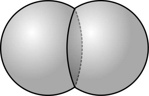 Figure 1
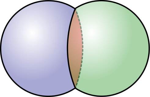 Figure 2
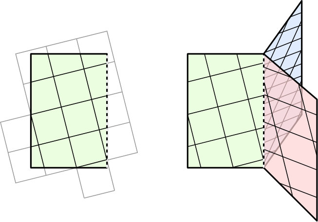 Figure 3
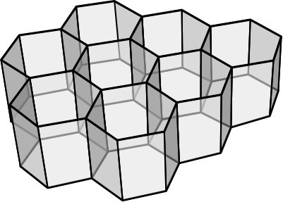 Figure 4
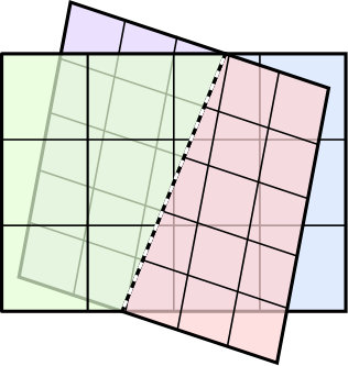 Figure 5
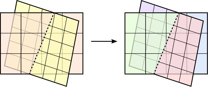 Figure 6
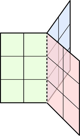 Figure 7
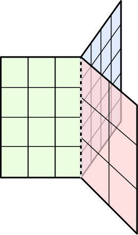 Figure 8
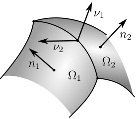 Figure 9
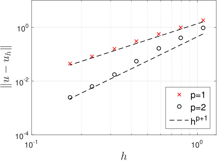 Figure 10
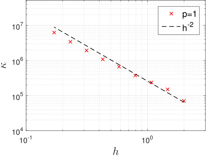 Figure 11
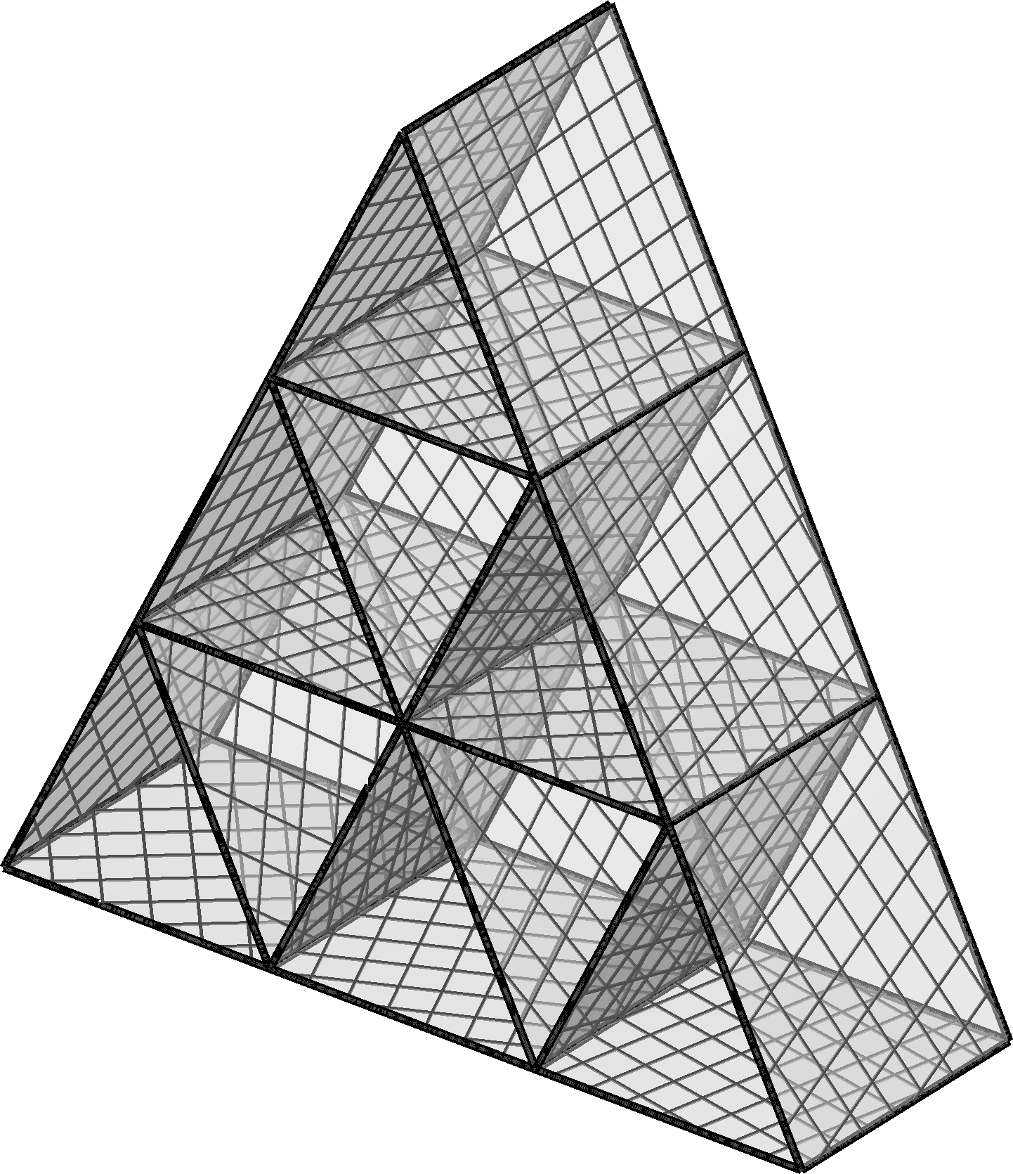 Figure 12
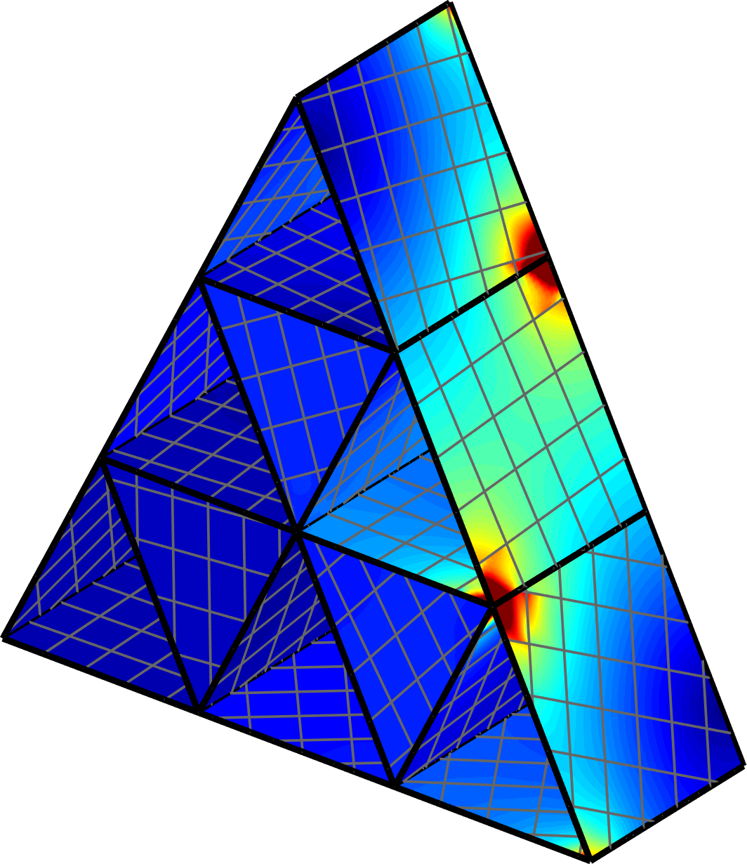 Figure 13
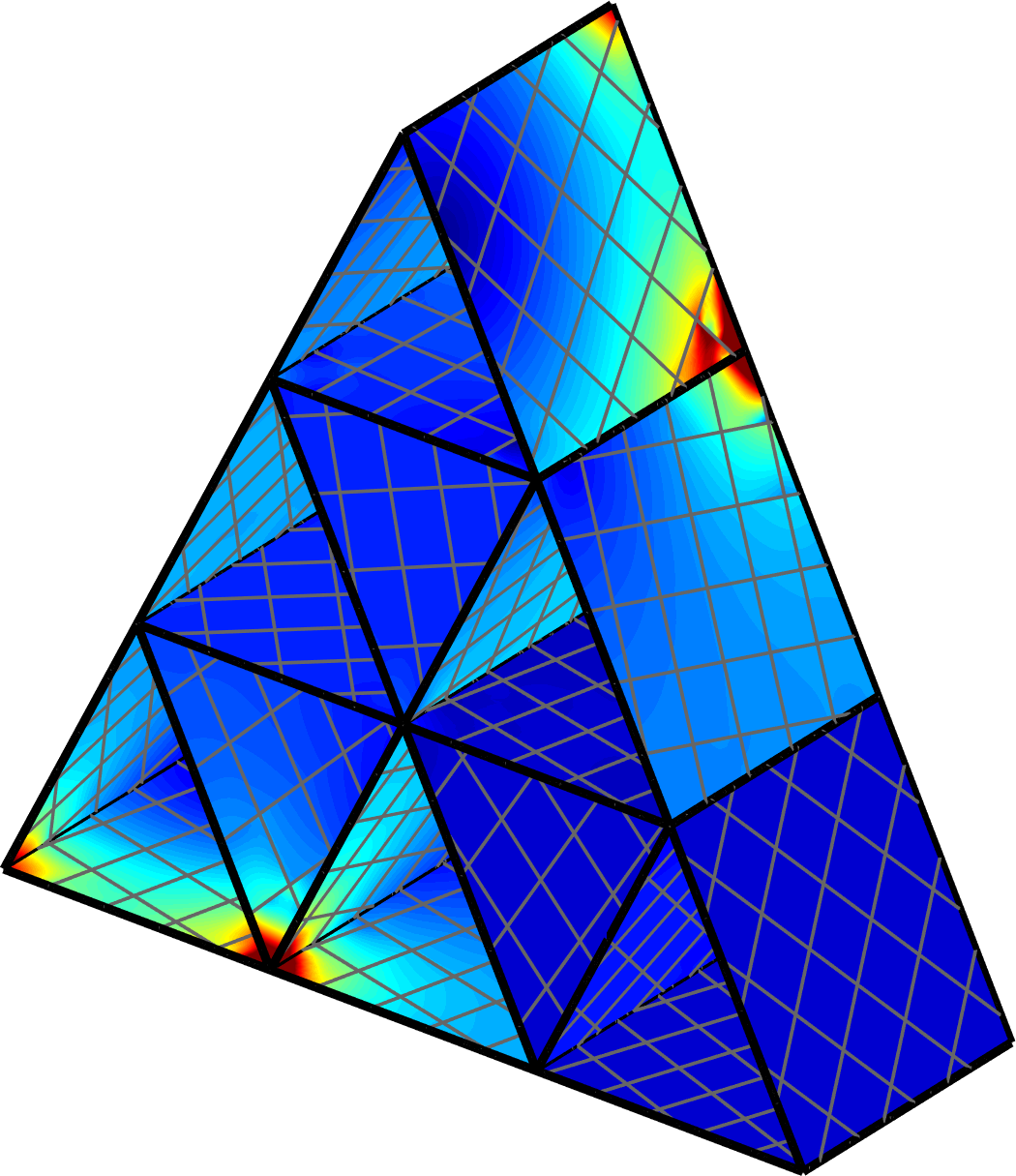 Figure 14
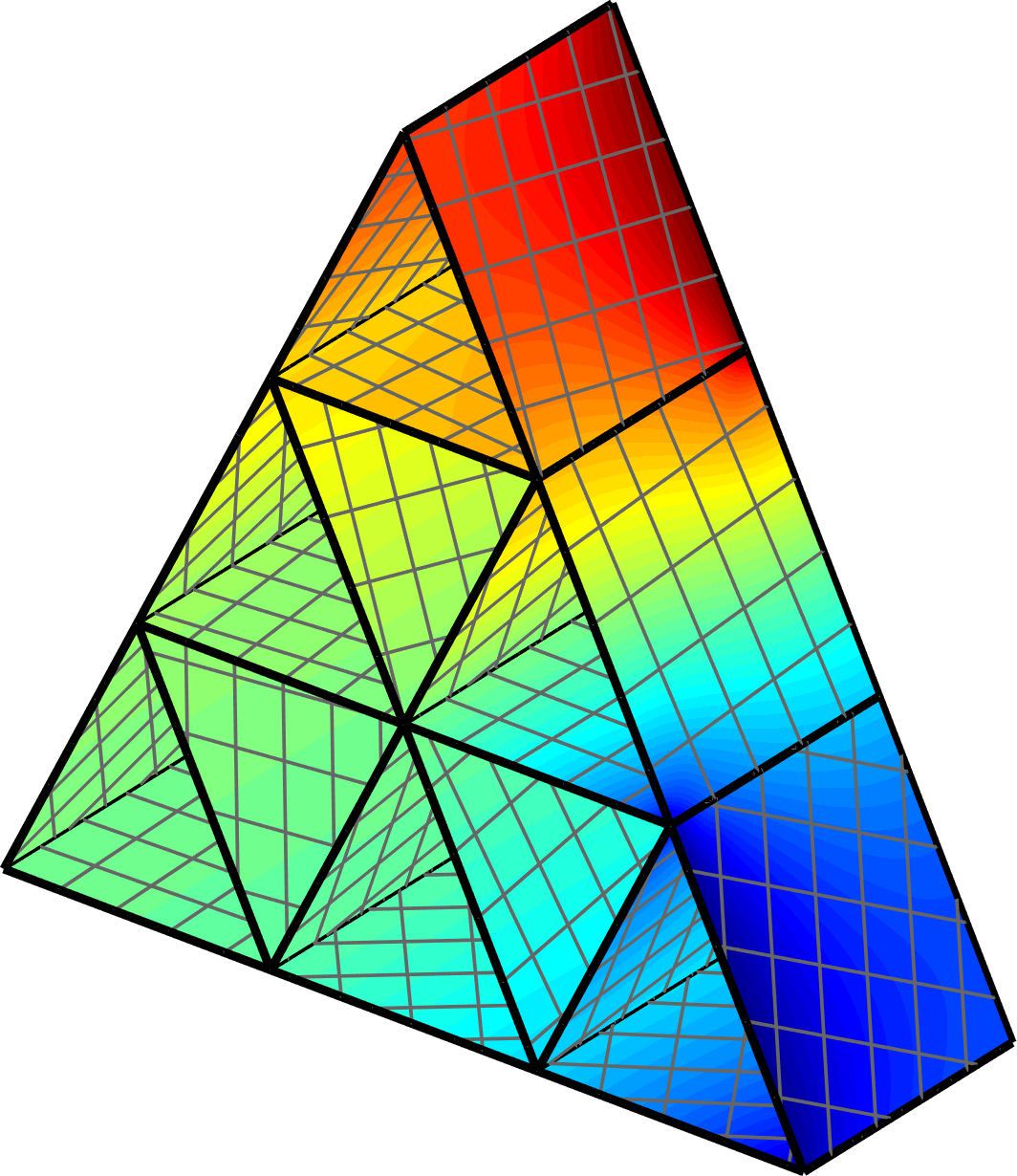 Figure 15
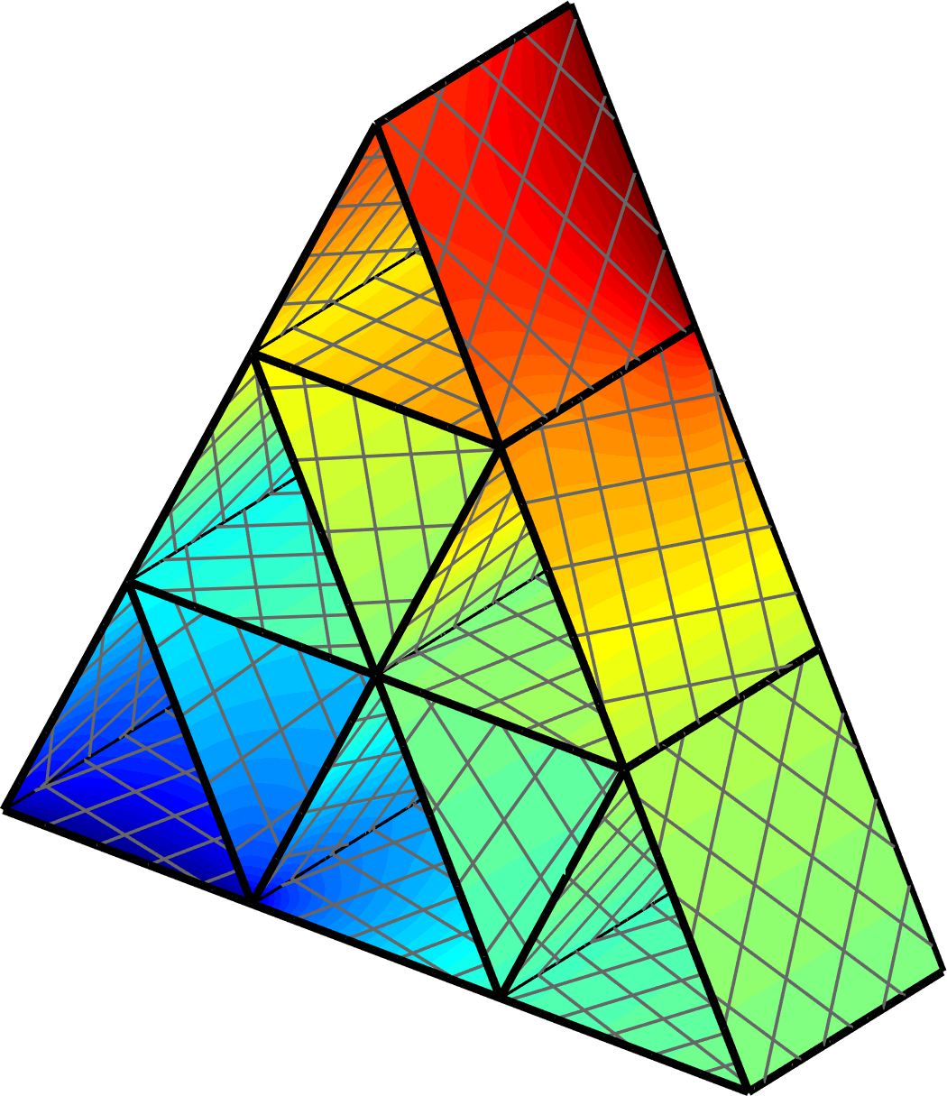 Figure 16
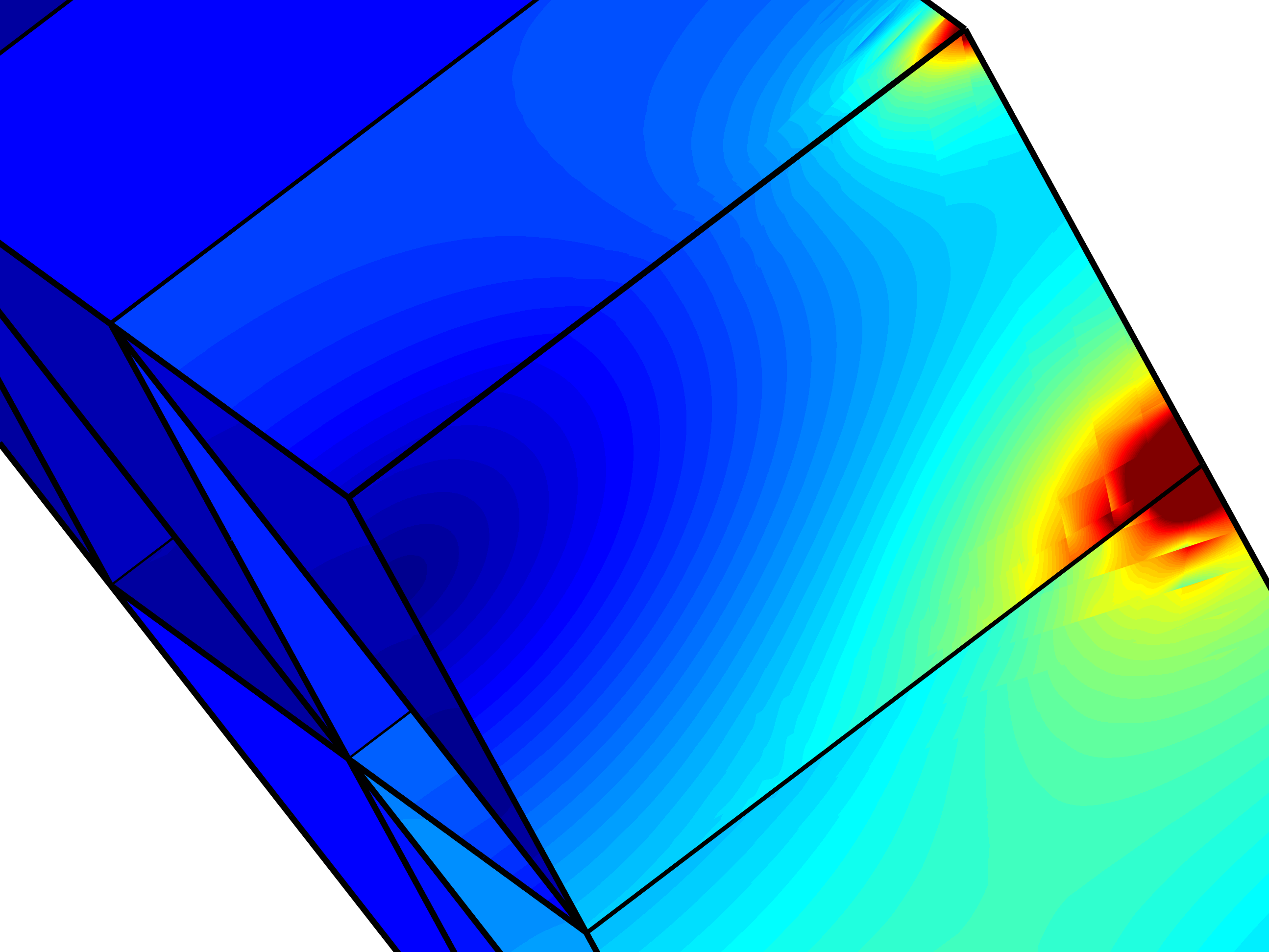 Figure 17
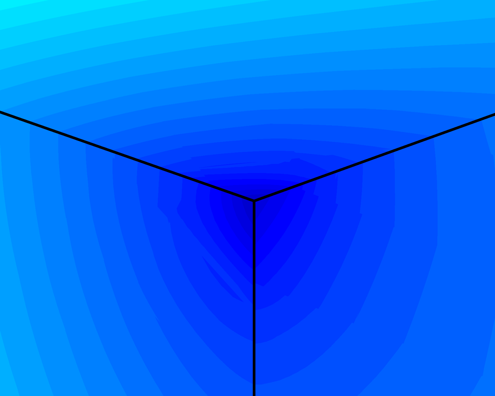 Figure 18
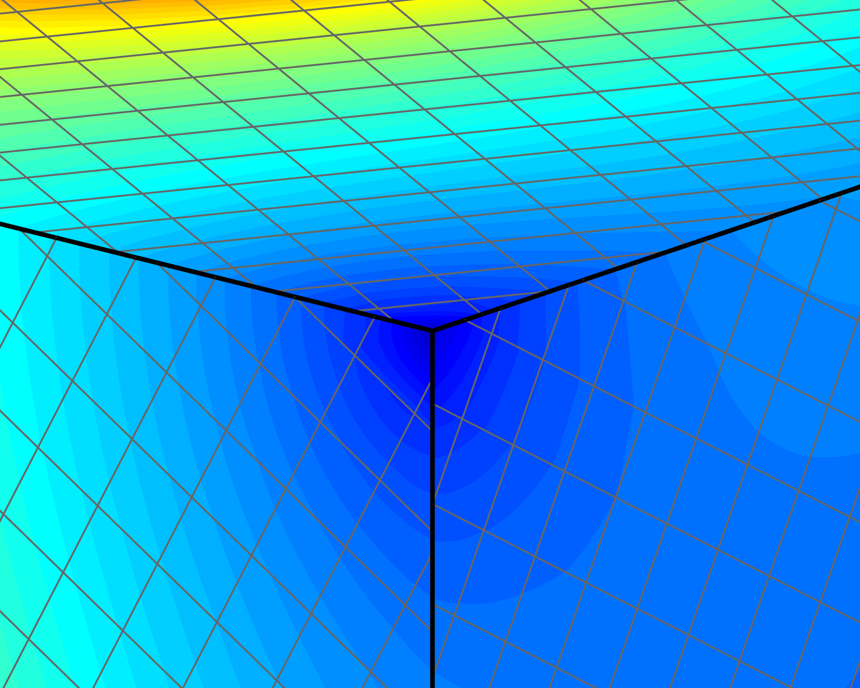 Figure 19
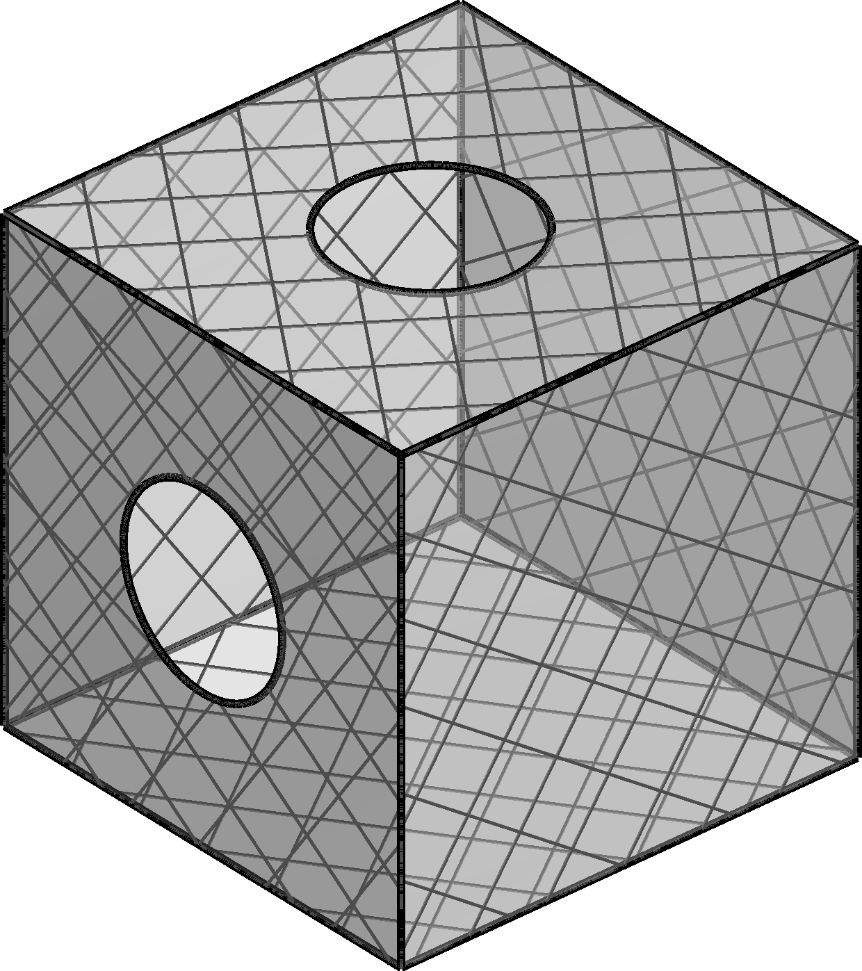 Figure 20
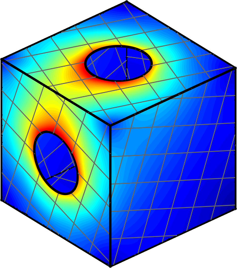 Figure 21
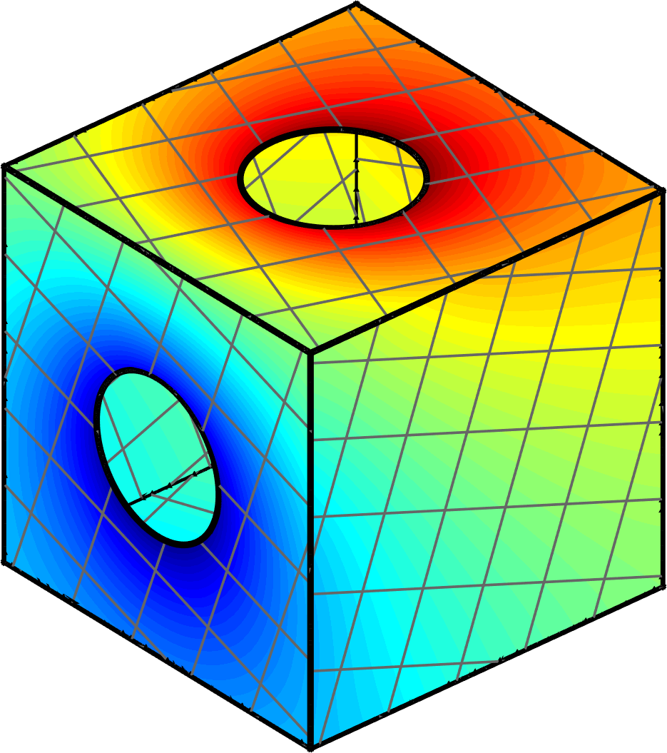 Figure 22
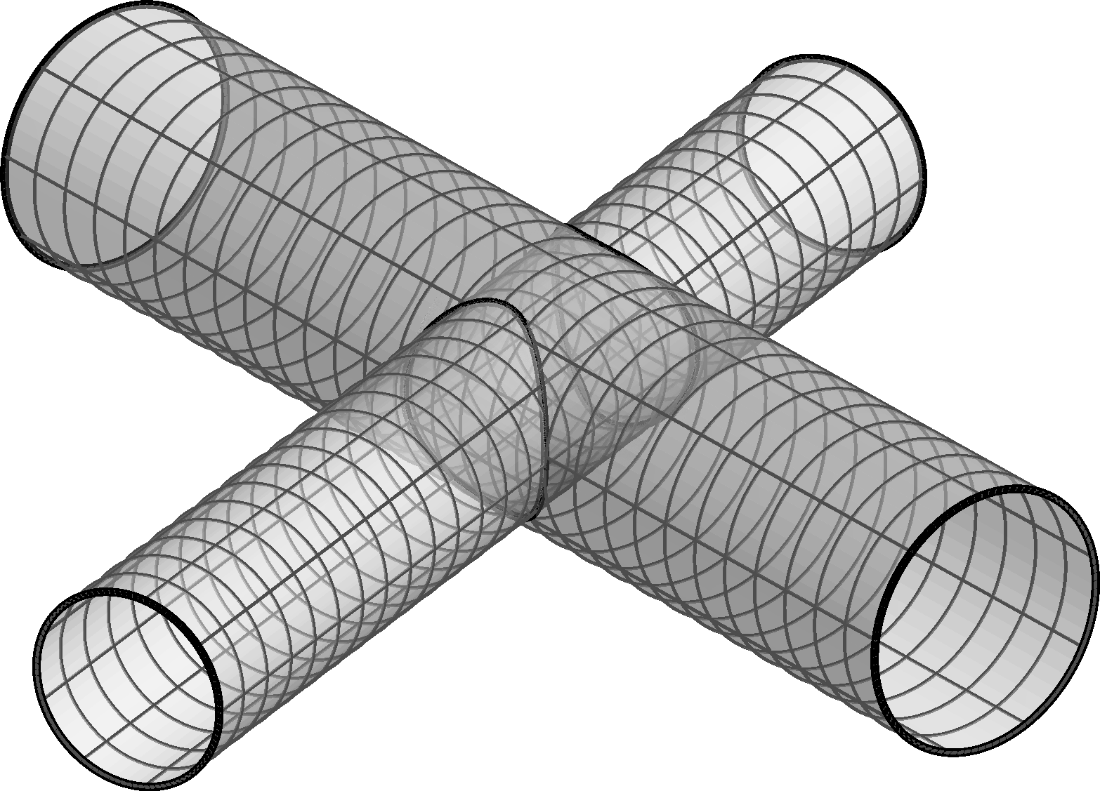 Figure 23
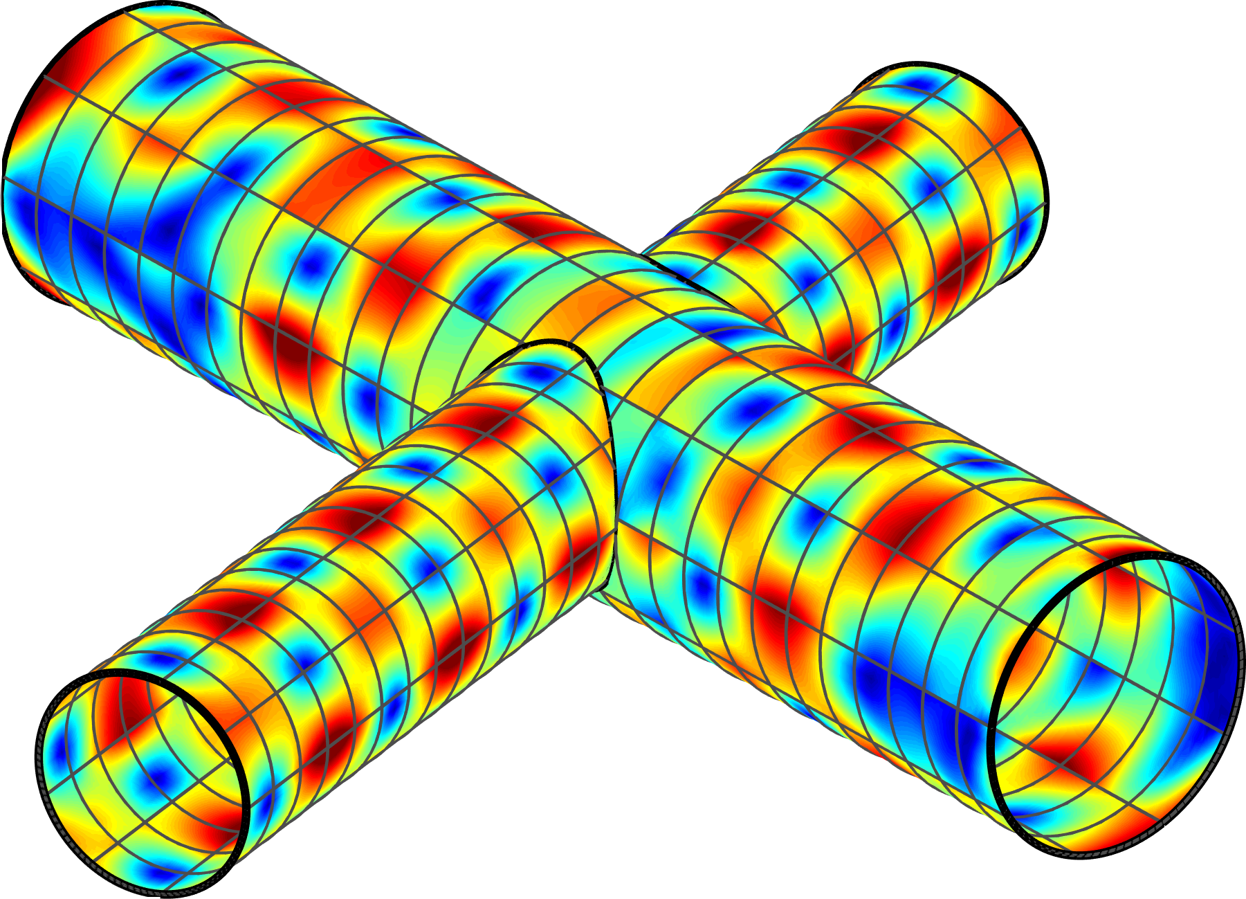 Figure 24
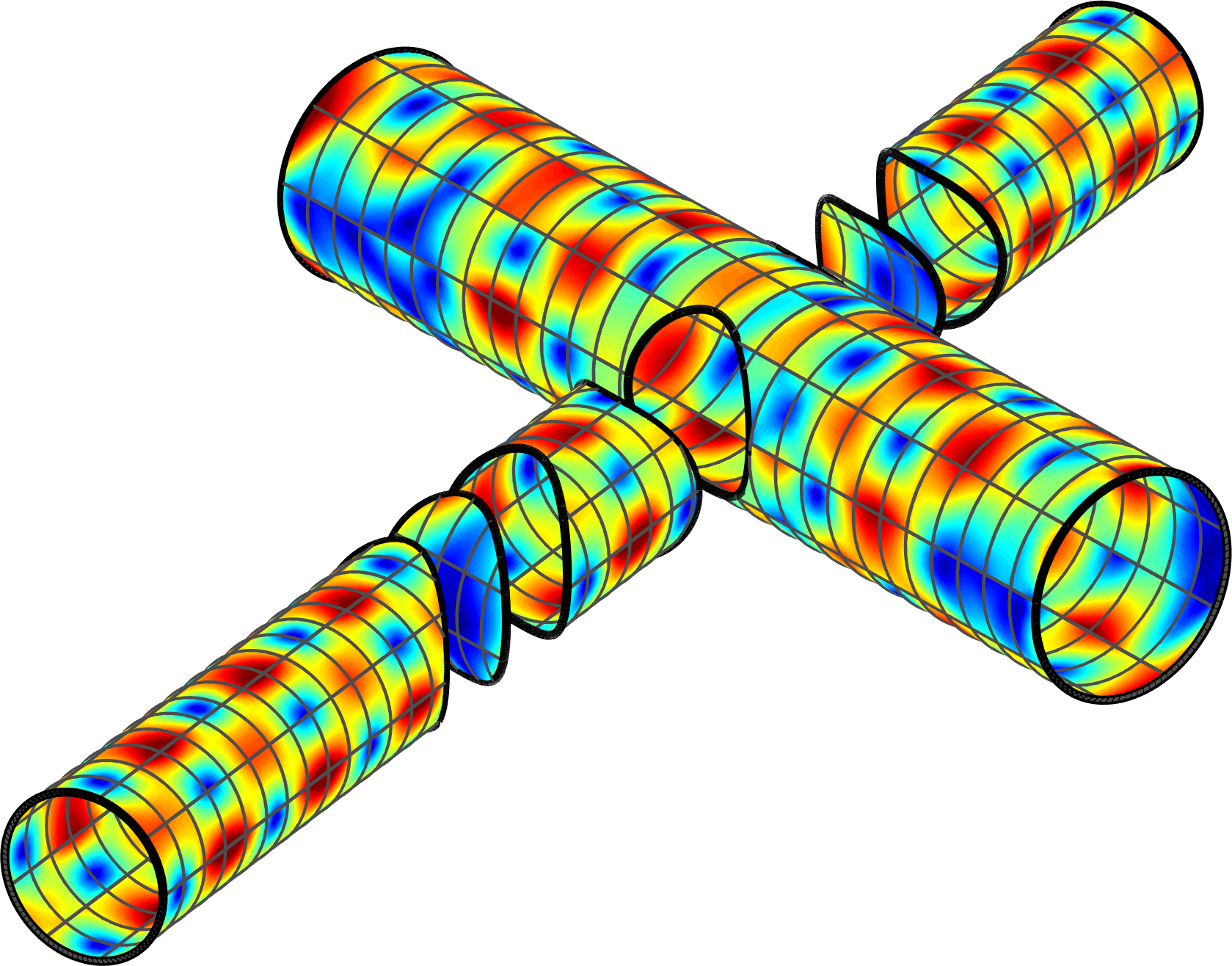 Figure 25
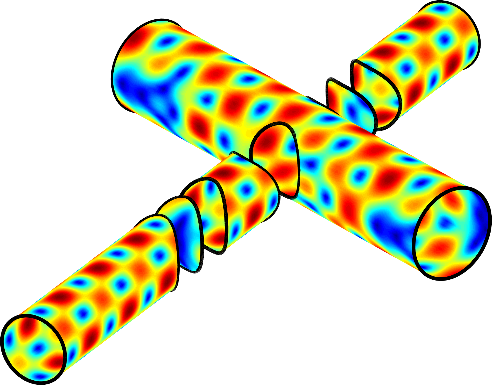 Figure 26
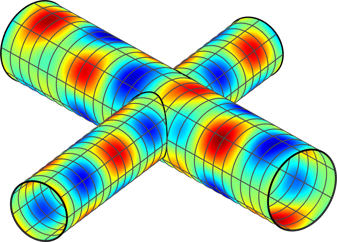 Figure 27
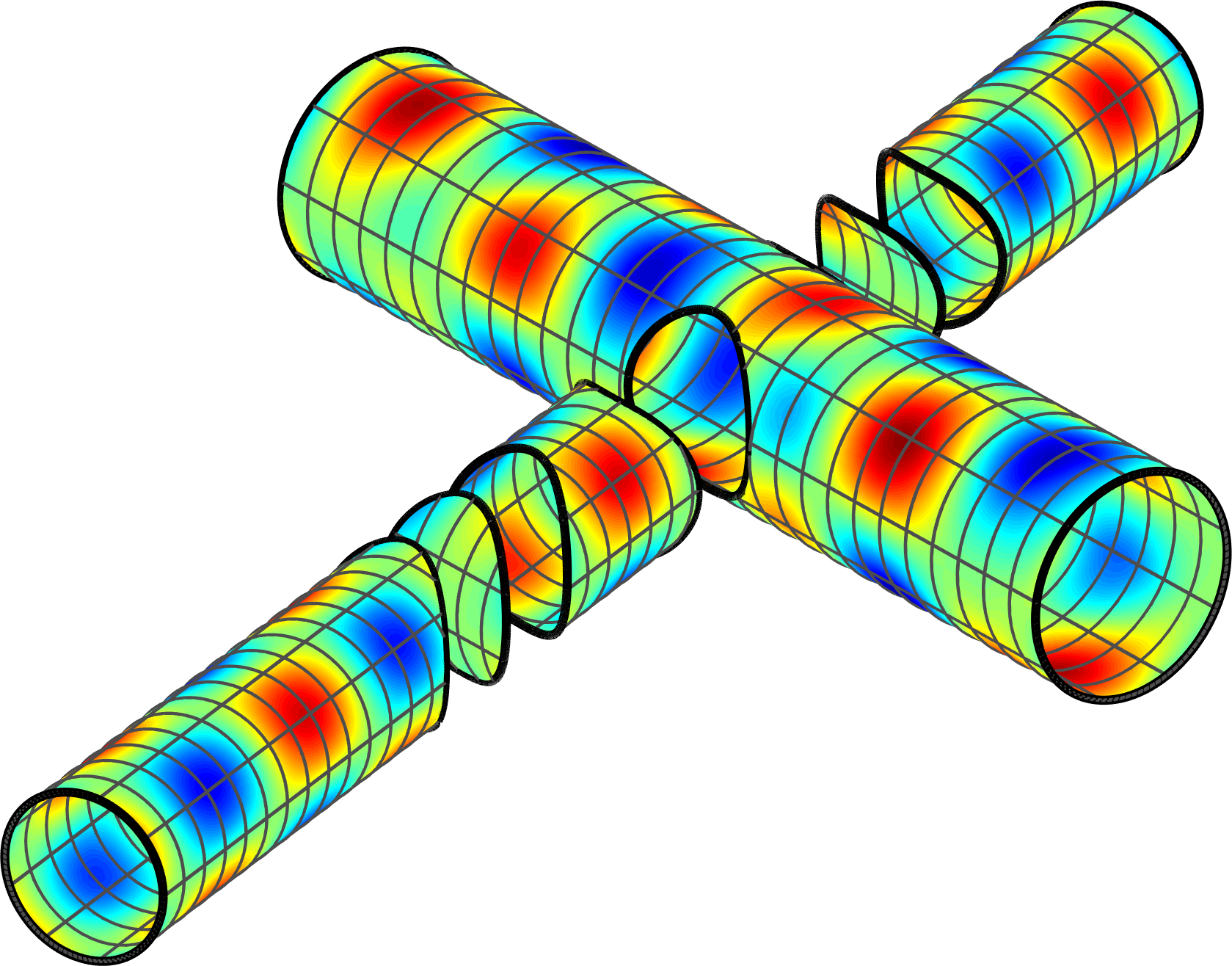 Figure 28
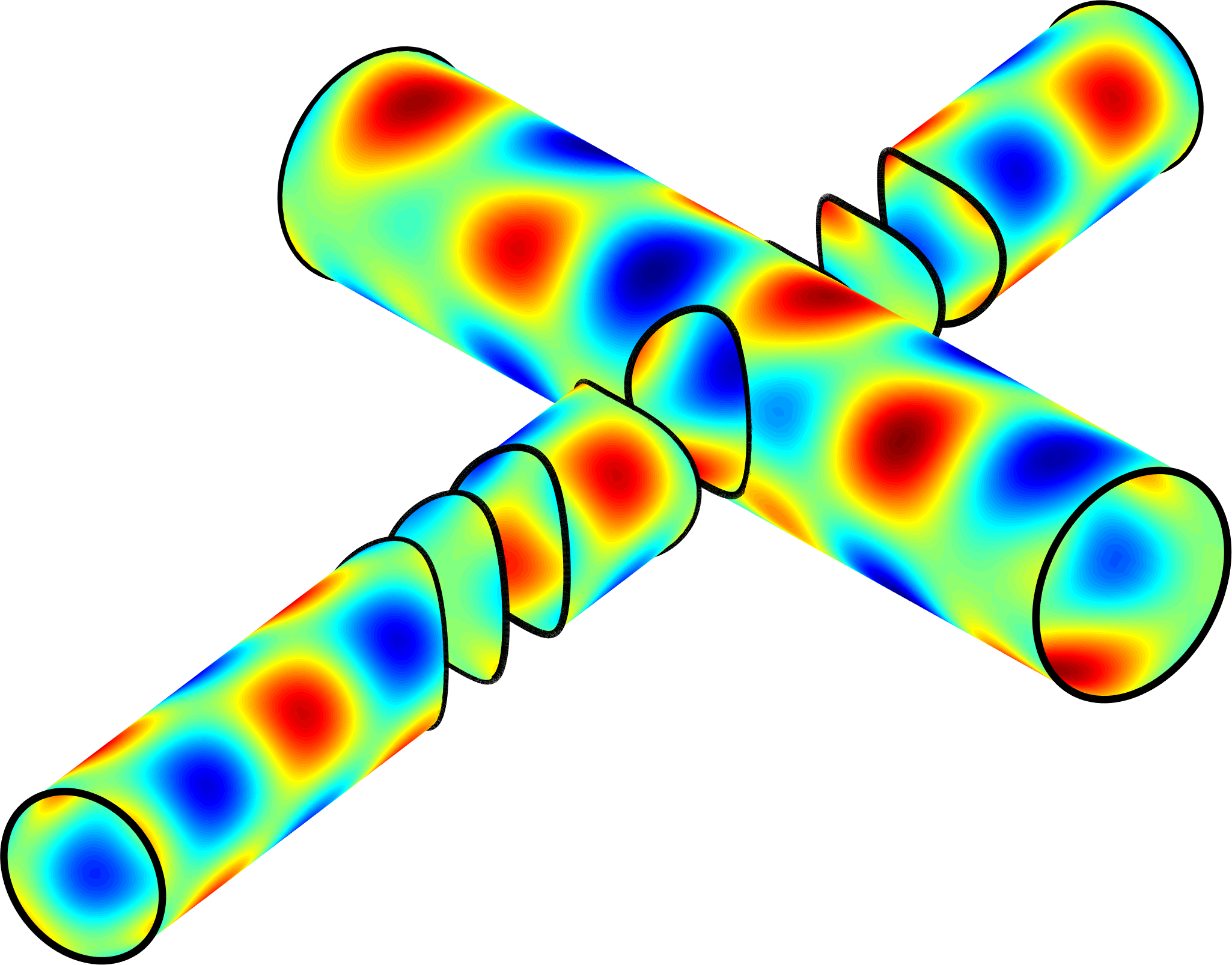 Figure 29
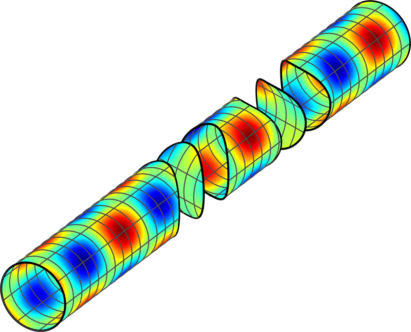 Figure 30
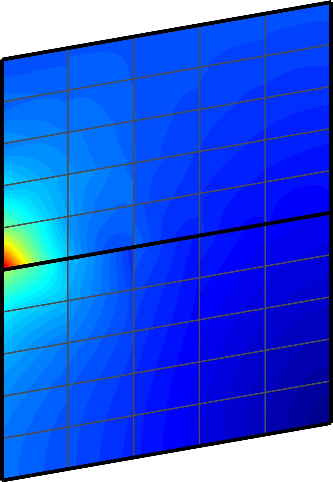 Figure 31
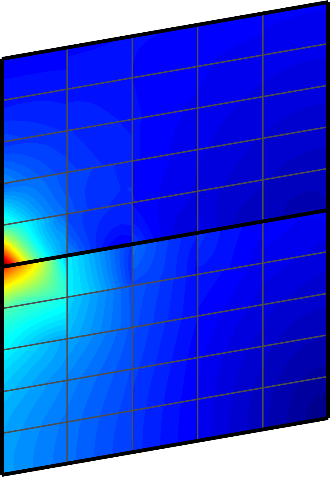 Figure 32
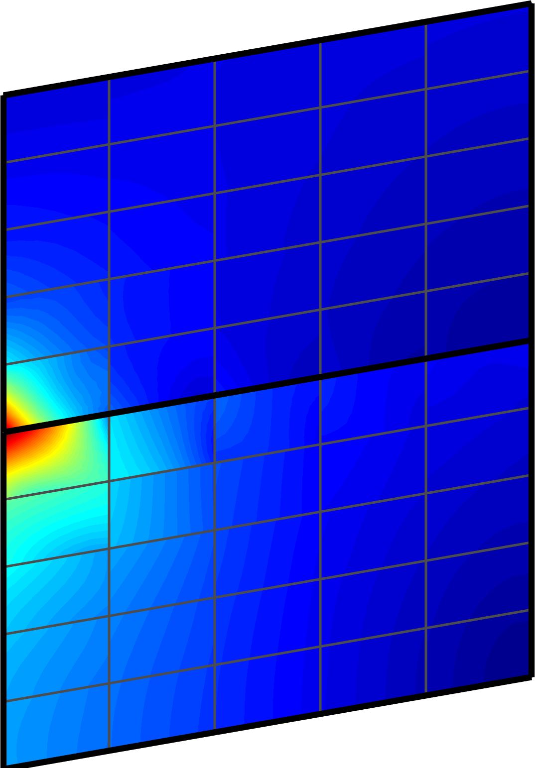 Figure 33
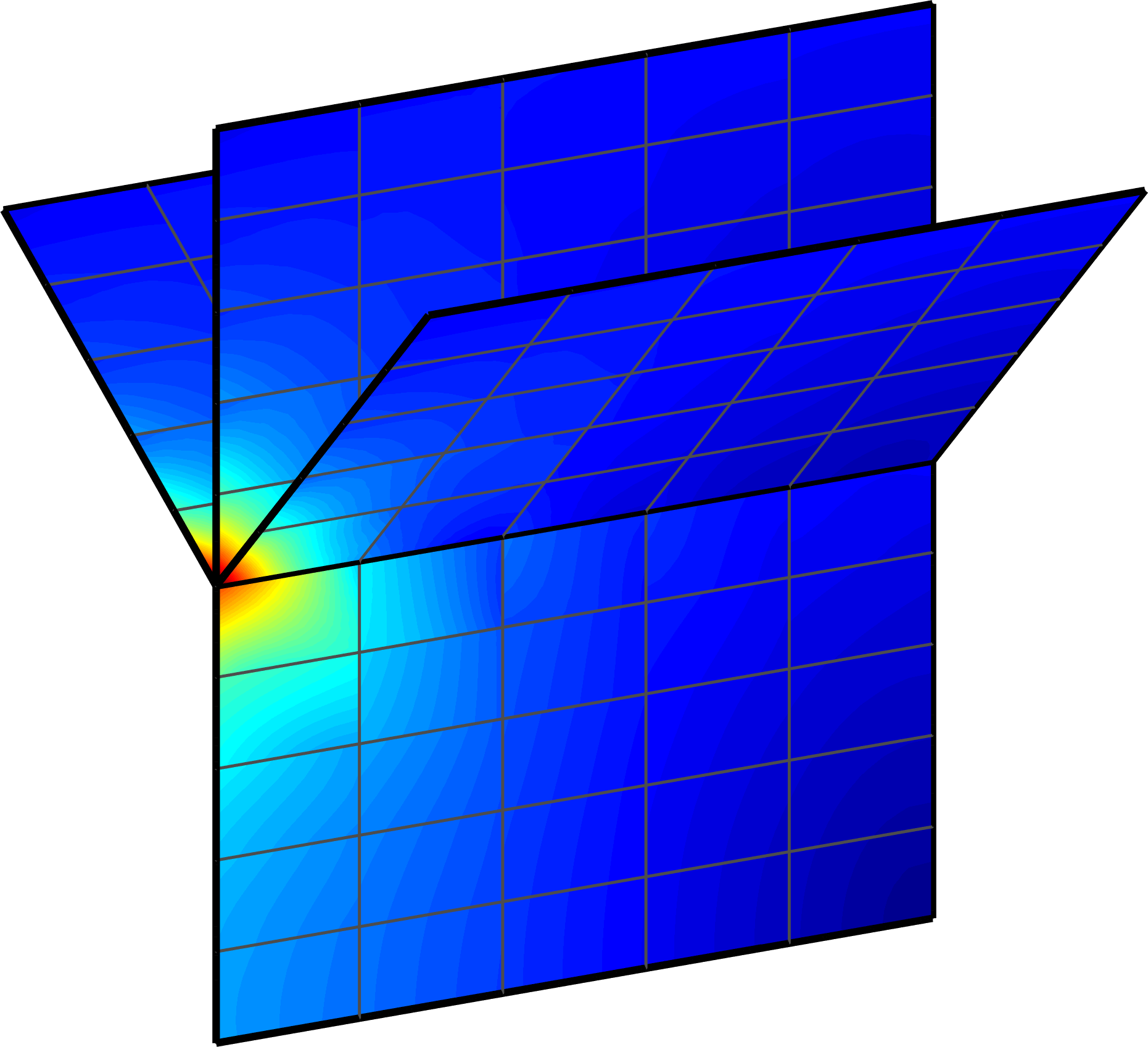 Figure 34
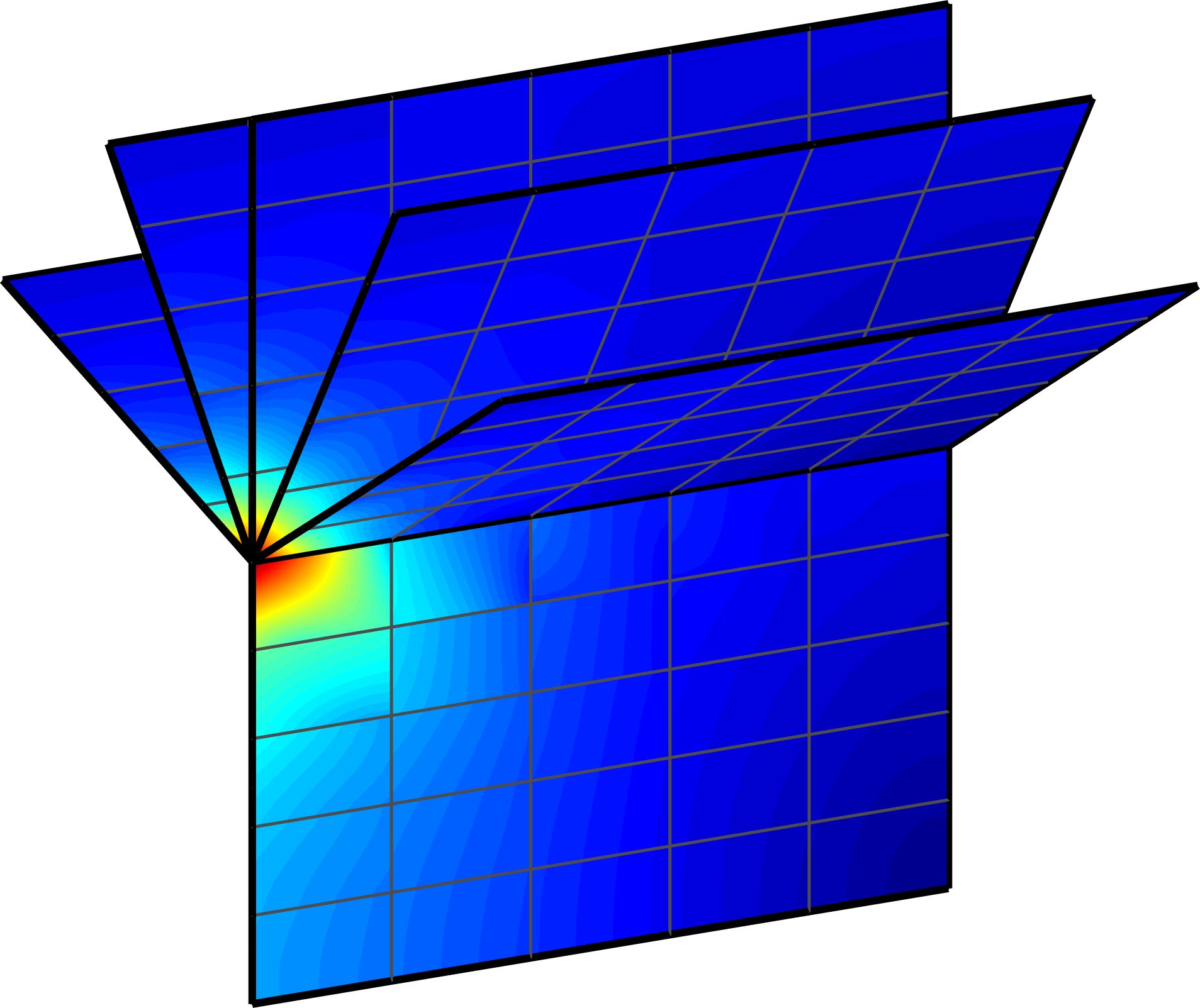 Figure 35
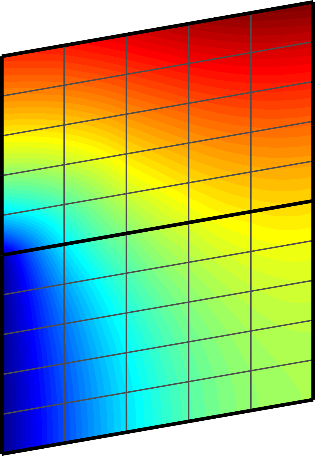 Figure 36
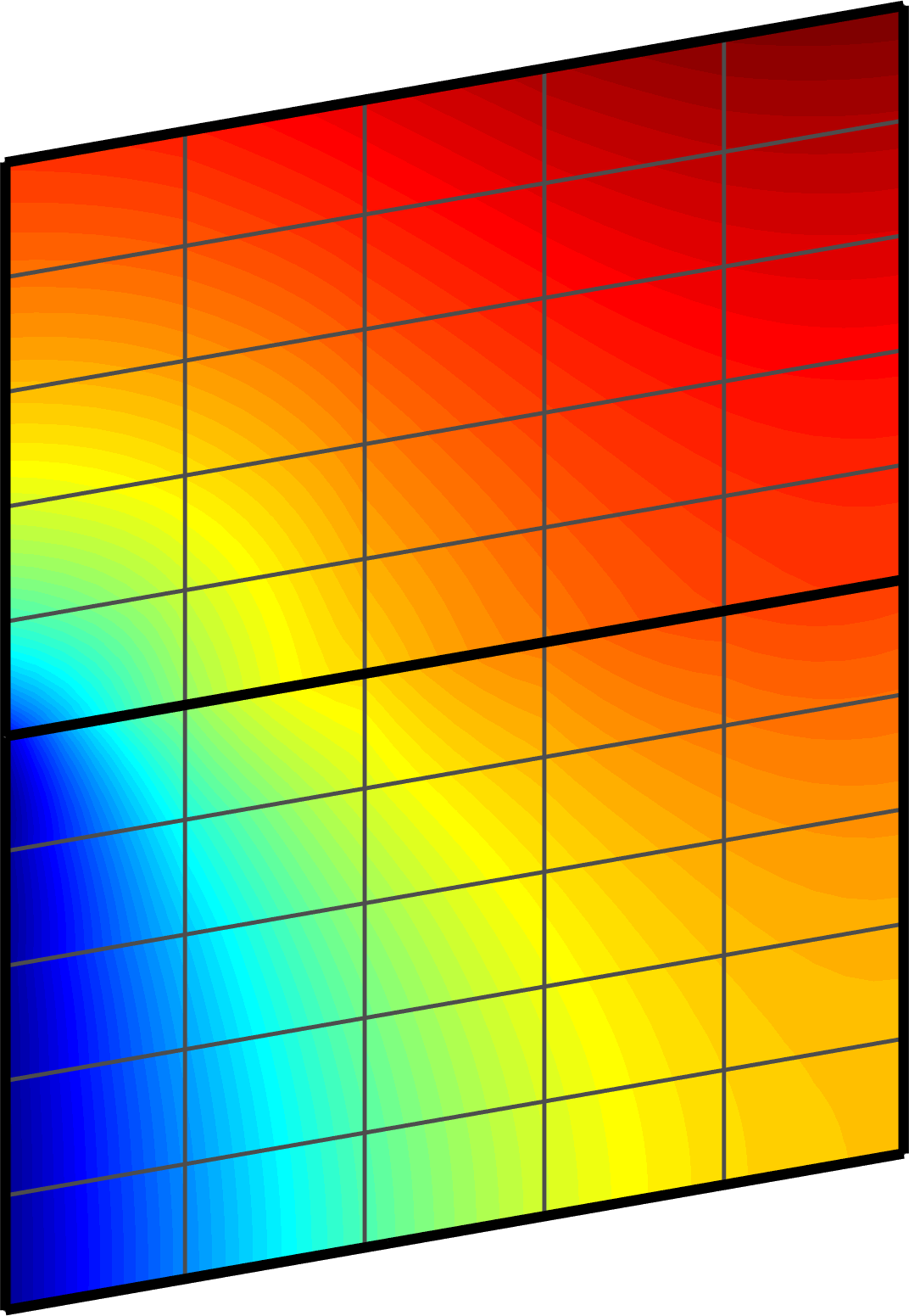 Figure 37
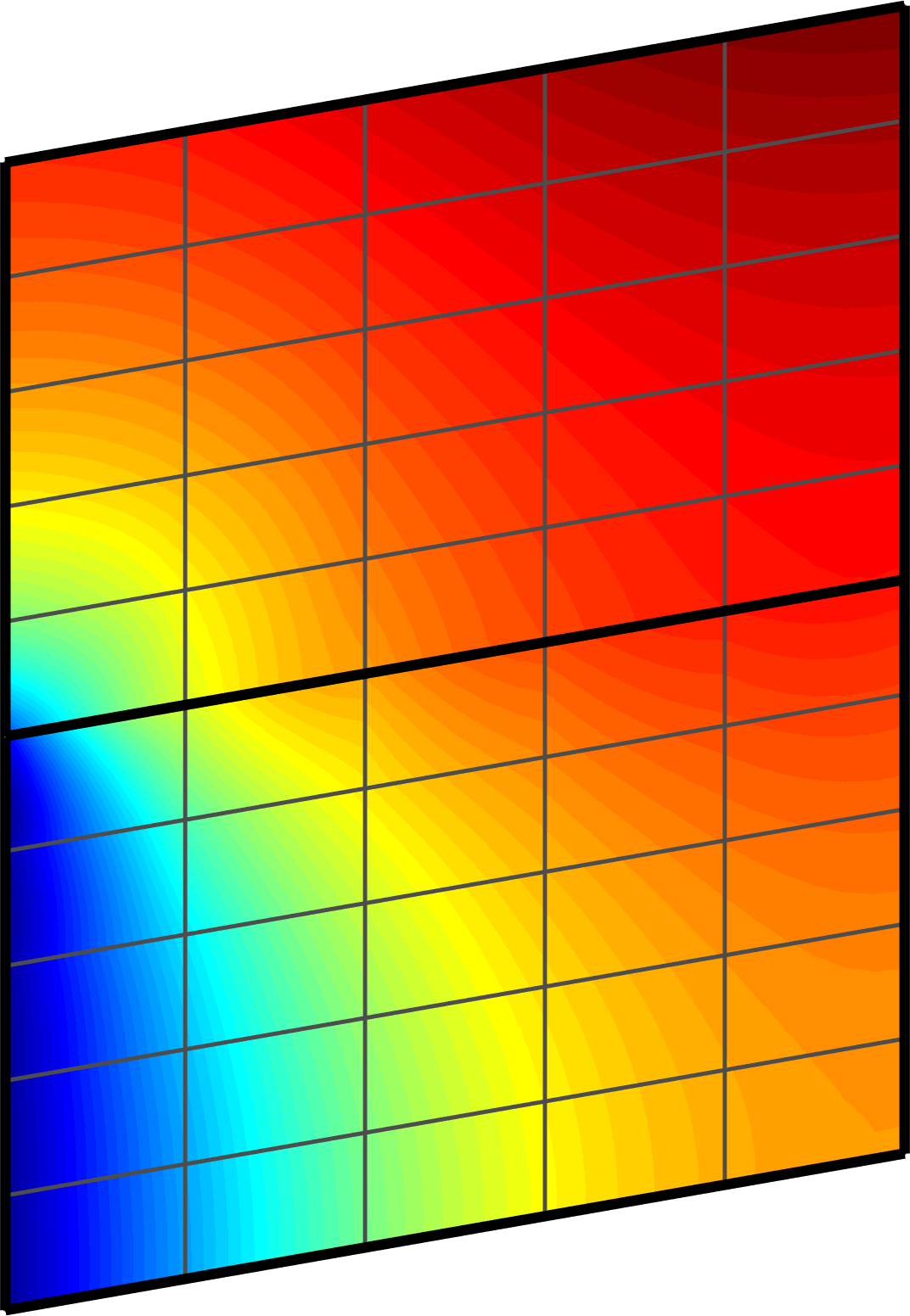 Figure 38
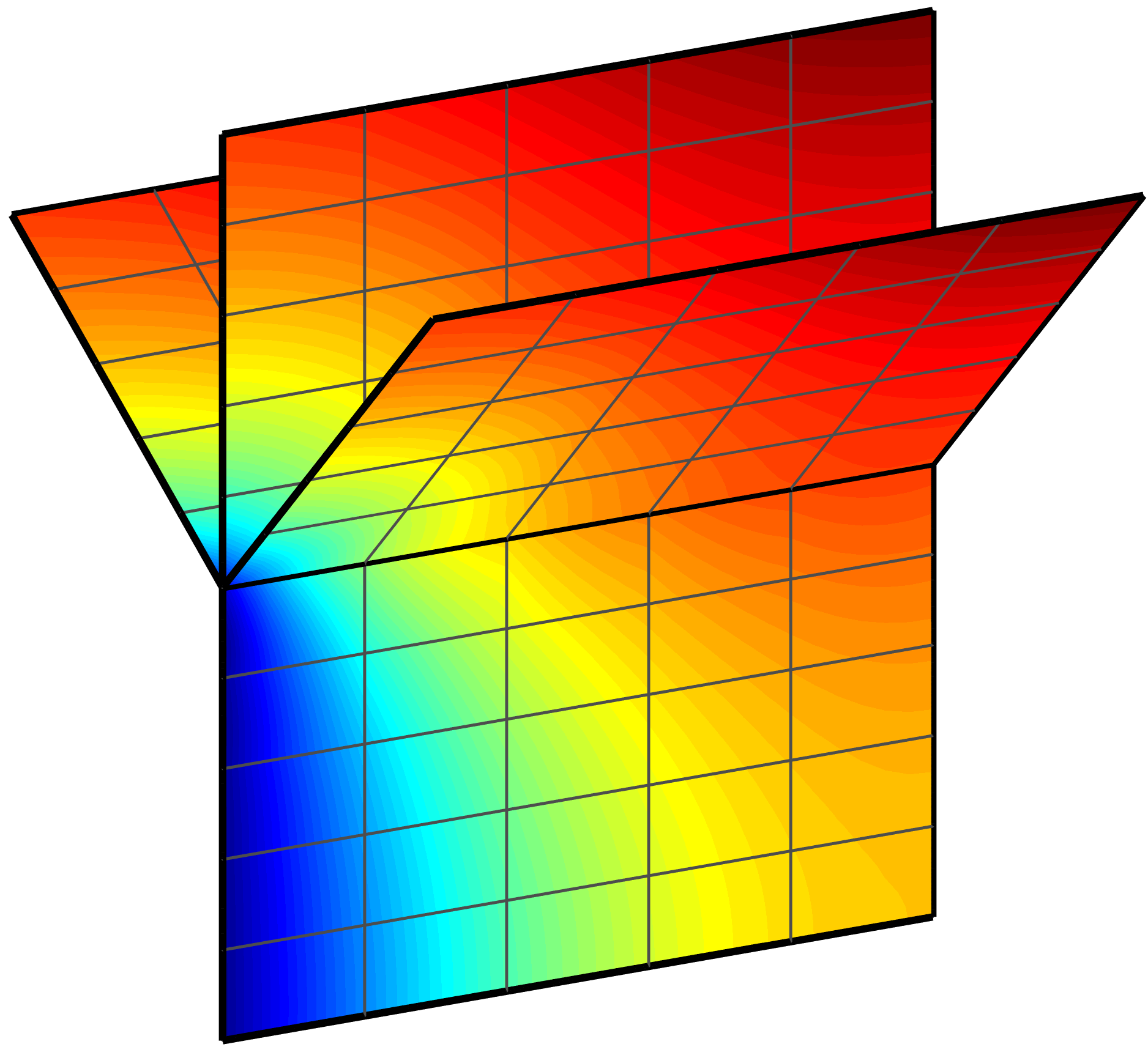 Figure 39
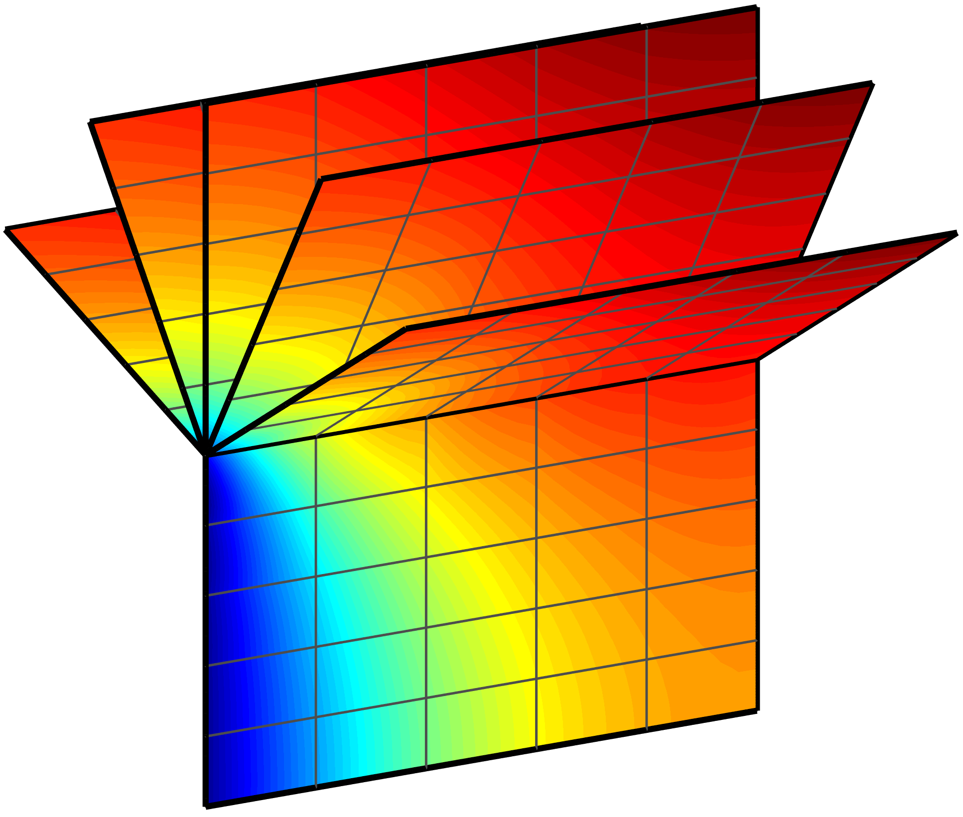 Figure 40
Peer Reviews
No public reviews on file for this paper yet. If you reviewed it on a platform where reviews are public (OpenReview, ICLR, NeurIPS, ICML), you can paste yours below so the community can read it here.
Videos
No videos yet. Explain this paper in a talk, walkthrough, or lecture? Add one.
A Nitsche Method for Elliptic Problems
on Composite Surfaces††thanks: This research was supported in part by the Swedish Foundation for Strategic Research Grant No. AM13-0029, the Swedish Research Council Grants Nos. 2011-4992, 2013-4708, the Swedish Research Programme Essence
Peter Hansbo 111Department of Mechanical Engineering, Jönköping University, SE-55111 Jönköping, Sweden.
Tobias Jonsson 222Department of Mathematics and Mathematical Statistics, Umeå University, SE-90187 Umeå, Sweden
Mats G. Larson 333Department of Mathematics and Mathematical Statistics, Umeå University, SE-90187 Umeå, Sweden
Karl Larsson 444Department of Mathematics and Mathematical Statistics, Umeå University, SE-90187 Umeå, Sweden
Abstract
We develop a finite element method for elliptic partial differential equations on so called composite surfaces that are built up out of a finite number of surfaces with boundaries that fit together nicely in the sense that the intersection between any two surfaces in the composite surface is either empty, a point, or a curve segment, called an interface curve. Note that several surfaces can intersect along the same interface curve. On the composite surface we consider a broken finite element space which consists of a continuous finite element space at each subsurface without continuity requirements across the interface curves. We derive a Nitsche type formulation in this general setting and by assuming only that a certain inverse inequality and an approximation property hold we can derive stability and error estimates in the case when the geometry is exactly represented. We discuss several different realizations, including so called cut meshes, of the method. Finally, we present numerical examples.
Contents
1 Introduction
Background.
Many physical phenomena takes place on geometries that consist of an arrangement of surfaces, for instance transport of surfactants, heat transfer, and flows in cracks. See Figure 1 for examples of surface arrangements. In manufacturing the use of surface arrangements to minimize the amount of needed material, for example in the form of honeycomb sandwich structures, is well established while recent developments of additive manufacturing enable production of even more complex surface structures. The arrangement of surfaces in applications often contain sharp edges, corners, and lines where several surfaces meet. Thus there is significant interest in the development of finite element methods for solving partial differential equations on such general geometries.
New Contributions.
In this contribution we develop a Nitsche method for a diffusion problem on a such an arrangement of surfaces. The key feature is that the formulation can handle interfaces where several surfaces meet at intersecting interfaces, including triple points and sharp edges. The method avoids defining a conormal to each interface and instead the well defined conormal associated with each subsurface is used together with the natural conservation law: the sum of all conormal fluxes is zero at the interface. This conservation law is sometimes refereed to as the Kirchhoff condition. We show that the method is equivalent to the standard Nitsche interface method in flat geometries. The same idea naturally extend to discontinuous Galerkin methods on surfaces, where instead of defining a conormal to each edge which would be needed in a standard discontinuous Galerkin method, see for instance the discussion in [6], the well defined discrete element conormal can be used.
We consider different ways of constructing a mesh on a composite geometry including matching meshes, non matching meshes, and cut meshes. For cut meshes we add a stabilization term that provides control in the vicinity of the interfaces. More precisely we consider a stabilization term, see [2] and [17], that satisfies certain abstract conditions which enable us to prove discrete stability and a priori error estimates. For clarity we restrict our analysis to the case when the geometry is exactly represented. This can be realized using parametric mappings, see [17]. We also give a concrete construction of such a stabilization term based on penalization of jumps in derivatives across faces belonging to elements that intersect the interface. We conclude the paper with some illustrating numerical examples.
Earlier Work.
Since the pioneering work of Dziuk [9] where a continuous Galerkin method for the Laplace-Beltrami operator on a triangulated surface was first proposed there has been several extensions including adaptive and higher order methods, Demlow and Dziuk [8] and Demlow [7], and higher order problems, Clarenz et al. [3] and Larsson and Larson [20]. A standard discontinuous Galerkin method for the Laplace–Beltrami operator on a smooth closed surface was analyzed in [6]. For further extensions including time dependent problems we also refer to the review articles [5, 10]. Models of membranes were considered in [13] and [15]. All of these contributions deals with smooth surfaces and the discontinuous Nitsche formulation proposed in this paper which allows more complex surfaces appears to be new. In [14] we develop a method for plate structures on composite surfaces consisting of plane surfaces with the restriction that only two plates meet at an interface. Here each plate is modeled using a membrane model and a fourth order Kirchhoff model for the bending. Various methods for connecting parametric patches pairwise which also allow for cut meshes have been proposed, see for example [19, 21, 18] and the extension to surfaces in [17].
Outline.
The outline of the remainder of the paper is as follows. In Section 2 we give a short introduction to tangential calculus on surfaces and then we formulate the model problem. In Section 3 we derive the method, study how it relates to the standard discontinuous Galerkin method in the the case of an interface in flat geometry, and introduce the stabilization term. In Section 4 we prove a priori error estimates in the energy and norm. Finally, in Section 5 we present some numerical examples illustrating the method on three different test cases.
2 Model Problem
2.1 The Composite Surface
Surface with Boundary.
Let be smooth surface embedded in with orientation (or normal) and boundary , which has the following properties
- •
There is a smooth closed surface embedded in such that .
- •
The boundary consists of a finite set of smooth curve segments and corner points . The exterior unit conormal to is denoted by .
- •
At each corner on the boundary there is a constant such that
[TABLE]
where denotes the left and right conormal at the corner .
Composite Surface.
We introduce the following notation:
- •
Let be a set of smooth surfaces with boundaries that satisfy the assumptions above.
- •
A composite surface is a finite union of surfaces with boundaries
[TABLE]
- •
The intersection between any two surfaces and , , is either empty or occur at the boundary of the surfaces,
[TABLE]
and is either a smooth curve segment (an interface curve) or a point (an interface node). Furthermore, given two surfaces and , there is a sequence of surfaces which starts with and end at such that two consecutive surfaces share a nonempty interface. This means that no surface share only a point with the union of the other surfaces.
- •
We may also assume that is one of the curve segments in and , if not we may simply modify the boundary description.
- •
Let be the set of all non-overlapping interface curves, for , such that
[TABLE]
Thus the union of the non-overlapping interface curves in includes all interface curves (2.3).
- •
Given an index we let be the set of indexes corresponding to surfaces that share interface .
2.2 Elliptic Model Problem
Notation.
We introduce the following notation:
- •
The tangential gradient is defined by , where is the projection onto the tangent plane of .
- •
is a given function such that with , and there are constants such that for all it holds
[TABLE]
- •
The flux is defined by
[TABLE]
Model Problem.
Consider the problem: find such that
[TABLE]
and that the following interface and boundary conditions are satisfied:
- •
For each the following interface conditions hold
[TABLE]
The first condition is a so called Kirchhoff condition and corresponds to conservation over interfaces while the second condition corresponds to continuity at the interface. Note that (2.8) thus encompasses the case where the interface is a sharp edge such as illustrated in Figure 2.
- •
The following boundary conditions hold
[TABLE]
where the boundary is decomposed into a Neumann boundary and a Dirichlet boundary such that , and .
2.3 Weak Form
Function Spaces.
Let
[TABLE]
be equipped with the inner product and associated norm
[TABLE]
Then is clearly a Hilbert space.
Derivation of Weak Form.
Starting from (2.7) and using Green’s formula on each of the surfaces in we obtain for ,
[TABLE]
where we used the identity on and on as well as the continuity for any and the interface condition (2.8) to conclude that
[TABLE]
Thus we arrive at the following weak problem: find such that
[TABLE]
where
[TABLE]
Existence and Uniqueness.
The form is coercive in and thus in case existence and uniqueness of the solution follows directly from the Lax-Milgram lemma. If we let be an extension of , set , where is determined by for all . Here we can again apply the Lax-Milgram lemma.
Regularity of the Solution.
As the assumptions in Section 2.1 allow for very intricate surface configurations it is challenging to give any precise prediction on the regularity of the solution . However, motivated by the regularity properties of elliptic problems in planar domains with nonsmooth boundary, see for example [11], we assume that
[TABLE]
where .
3 The Finite Element Method
In this section we derive our finite element method on the composite surface . For clarity we consider the situation when is exactly represented, which may be realized using exact parametric mappings. In the case of domains described by CAD models, the underlying assumption in isogeometric analysis, see [16, 4], the surface is equipped with a parametric finite element space consisting of continuous functions without any continuity requirement across the interface curves. In this setting we can focus on essentials and derive the method together with the basic properties including a stability result and an priori error estimate.
3.1 Constructions of Meshes on Composite Surfaces
There are several different natural ways to construct a mesh on a composite surface:
- (a)
Each surface is meshed with elements and matching meshes are used across the interface curves. 2. (b)
Each surface is meshed with elements and non matching meshes are used across the interface curves. 3. (c)
A number of surfaces are individually meshed and arranged in such a way that they intersect. In this situation so called cut elements naturally occur close to the interface. 4. (d)
Each of the surfaces is meshed using a cut finite element technique.
Examples of these mesh constructions are illustrated in Figure 3. In the case of cut elements we add a stabilization term which enables us to prove stability and optimal order error estimates.
The Mesh.
To accommodate these different situations we define the mesh as follows. For each we assume that there is a family of quasi uniform meshes with mesh parameter such that
[TABLE]
and
[TABLE]
The mesh may match perfectly, i.e, we could have equality in (3.1).
3.2 The Finite Element Spaces
Finite Element Space.
Let denote the space of either full or tensor product polynomials of degree less or equal to on . For each mesh there is a family of finite element spaces , , such that for all . On the composite surface we define the broken finite element space
[TABLE]
Approximation Property.
For each there is an interpolation operator such that
[TABLE]
and on the composite surface we have the interpolation operator such that for . See [17] for the construction of such an interpolation operator in the case of cut meshes.
3.3 The Method
Derivation.
For we obtain using Green’s formula
[TABLE]
Conservation (2.8) states that for each ,
[TABLE]
which implies
[TABLE]
where is the convex combination
[TABLE]
with and . We may thus subtract in the interface term as follows
[TABLE]
Next for each we add the consistent stabilization term
[TABLE]
where is a positive parameter.
We may also symmetrize the method by adding a consistent term and the Dirichlet boundary is taken care of using a standard Nitsche formulation.
The Method.
Find such that
[TABLE]
where
[TABLE]
and
[TABLE]
3.4 Relation to the Standard Average-Jump Formulation
Consider an interface curve which has only two neighboring surfaces and assume that is a positive constant. We may assume that . Then we have
[TABLE]
and the concistency term takes the form
[TABLE]
where is the jump in across and
[TABLE]
is the average of the normal flux. Note, that in the case when and are tangent at we have and we find that
[TABLE]
which is the usual average in discontinuous Galerkin methods. Note, in particular, that our formulation thus extends the standard discontinuous Galerkin formulations to surfaces with sharp edges. Finally, we easily find that the penalty term takes the form
[TABLE]
where we used the assumption that is constant and the identities and . We conclude that the penalty term is of the same form as in the standard discontinuous Galerkin interior penalty term.
3.5 The Stabilization Term
Abstract Properties.
In the case of cut elements at an interface we add a stabilization term of the form
[TABLE]
where is a positive semidefinite bilinear form on , and define the stabilized form
[TABLE]
and the following seminorms on each subsurface
[TABLE]
We assume that the stabilization term has the following properties:
- •
There is a constant such that for all and it holds
[TABLE]
- •
There is a constant such that for all and with it holds
[TABLE]
Here and below we use the abbreviated notation for the inequality where is a constant independent of the mesh size parameter .
Remark 3.1
In order to prove a bound on the condition number of the stiffness matrix we assume that
[TABLE]
The condition number bound can then be proved using the techniques in [17].
Remark 3.2
Note that we do not assume that the stabilization form is consistent, i.e. for the exact solution , for , even though this may be the case for a sufficiently regular solution.
Normal Derivative Jump Penalty.
The stabilization form which we will use in this paper takes the form
[TABLE]
where is the set of interior faces in the mesh , which belong to at least one element such that . We note that is consistent for sufficiently regular functions, for instance for we have for .
We first note that is a bilinear positive semidefinite form by construction. To verify (3.29) we recall, see [17] Lemma 4.1, that for two neighboring elements and in which share the face we have the estimate
[TABLE]
and we may conclude that, for with small enough,
[TABLE]
where is the set of elements that do not intersect the boundary. Finally, we have the inverse estimate
[TABLE]
where is the set of elements that intersect the boundary in a face or in the interior. See [12] for the trace inequality , , from which (3.35) follows. Combining estimates (3.34) and (3.35) we find that
[TABLE]
To verify (3.30) we consider again the pair of two elements and sharing the face and we let . We note that and thus
[TABLE]
where we used an inverse inequality and the Bramble–Hilbert Lemma to estimate the second term. Summing over all and using the approximation property (3.4) give (3.30).
Least Squares Gradient Variation Penalty.
Define
[TABLE]
where is the projection. This stabilization term is not consistent but it is not difficult to verify that it satisfies the conditions (3.30) and (3.30) using similar arguments as above. See also [1] where related stabilization terms were studied.
4 Properties of the Finite Element Method
4.1 Coercivity and Continuity
We define the norms
[TABLE]
and
[TABLE]
where
[TABLE]
Lemma 4.1
For large enough penalty parameter , there is a constant such that for all it holds
[TABLE]
There is a constant such that for it holds
[TABLE]
and
[TABLE]
Proof. For large enough penalty parameter the coercivity follows from the fact that the inverse inequality (3.29) holds together with standard arguments.
4.2 Interpolation Error Estimate
We have the estimate
[TABLE]
This inequality follows from the trace inequality
[TABLE]
for each element , with a nonempty intersection with and the interpolation estimate (3.4).
4.3 Error Estimates
In the proof of the error estimate we will use a duality argument and we now specify the regularity properties needed for our analysis. Let be the solution to the dual problem
[TABLE]
where . We assume that there are constants , and a hidden constant such that for all , the regularity estimate
[TABLE]
holds.
Theorem 4.1** (Error Estimates)**
Assume that the exact solution to (2.20) satisfies the regularity estimate (2.22), then there is a constant such that
[TABLE]
with
If in addition the solution to the dual problem (4.9) satisfies the regularity estimate (4.10), then there is a constant such that
[TABLE]
where
Remark 4.1
Note that it follows from (4.11) and (3.30) that
[TABLE]
Proof. (4.11). Splitting the error into an interpolation error and a discrete error we have
[TABLE]
where we used the energy norm interpolation error estimate (4.7). Next using coercivity (4.4) we have
[TABLE]
Here the numerator may rewritten, using the definition of the method (3.13), , , and the fact that the unstabilized method is consistent , , as follows
[TABLE]
Thus we find that we have the bound
[TABLE]
where we used the energy norm interpolation estimate (4.7) and the approximation property (3.30) of . Combining (4.16) and (4.23), gives
[TABLE]
which together with (4.15) concludes the proof.
(4.12).
Let be the solution to the dual problem (4.9) with , where is the error. We note that by consistency we have
[TABLE]
Setting we obtain
[TABLE]
Here we used the energy norm bound (4.11) and the energy interpolation estimate (4.7) followed by the elliptic regularity bound (4.10) to conclude that the following estimate holds
[TABLE]
5 Numerical Examples
Geometries.
We demonstrate the method using the three composite surfaces illustrated in Figure 4, where each geometry has different features:
- •
The cube with holes in Figure 4(a) consists of 6 separate surfaces pairwise connected along 12 interface lines. The resulting compound surface feature both sharp edges and corners.
- •
The house of cards in Figure 4(b) consists of 18 separate surfaces and 10 interface lines. Here each interface connects 2-6 surfaces. Also this geometry has sharp edges.
- •
The intersecting cylinders composite surface in Figure 4(c) is constructed by intersecting two cylinder surfaces and cutting the surfaces along their intersection. This construction produces 6 surfaces connected along the interface curves. In this geometry both the surfaces and the interfaces are curved and 4 surfaces meet at each interface.
General Construction.
All examples share the following set-up:
- •
The geometry of each surface is exactly described by a mapping , where is the reference domain and .
- •
The elements used in all examples are parametric quadratic tensor product Lagrange elements () and we allow cut elements at the interfaces. The parametrization is based on the exact map ,
[TABLE]
where is the finite element space in the reference domain. The stabilization term is evaluated in the reference domain, see [17] for further details.
- •
Our Nitsche penalty parameter is chosen to be and our stabilization parameter to be .
- •
We solve the model problem , where and , together with Dirichlet and Neumann boundary conditions.
5.1 Visual Examples
Cube with holes.
The cube illustrated in Figure 4(a) is an example of a composite surface which includes both sharp edges and corners. We consider our model problem with load and non-homogeneous Dirichlet boundary conditions. The boundary in this case consist of the two holes and we let along the top hole and along the side hole. We present a finite element solution and the magnitude of its gradient in Figure 5 using unfitted meshes on each surface. Note that as implied by the interface conditions (2.8)–(2.9) both the solution and the flux seem to flow continuously over the interfaces. Curiously, the gradient near the cube corners do not seem to include any singularity, as could possibly be expected, but is rather zero at the corner. We highlight this in Figure 6.
House of Cards.
The house of cards composite surface shown in Figure 4(b) includes interfaces joining more than two surfaces. Again we consider our model problem with and we set the non-homogeneous Dirichlet boundary condition on the right side of the top card closest in view and on the left side of the bottom standing card closest in view. On the remainder of the boundary we use homogeneous Neumann conditions. This leads to singularities in the points where we switch boundary conditions. Note that the singularities spread to the surfaces that couple at the interface. However, as the Kirchhoff condition (2.8) states that the sum of the conormal fluxes should be zero we no longer have pairwise continuity of fluxes over interfaces joining more than two surfaces. We can see this in Figure 8 where we also note the peculiar effect that the singularities due to the switch of boundary condition at the interfaces has a greater effect on interfaces joining more surfaces. While somewhat counter intuitive we isolate this effect in the study presented in Figure 9.
5.2 Convergence
Intersecting Cylinders.
Here we consider the composite surface constructed by intersecting two cylinders with radii and cutting the surfaces along the intersection as shown in Figure 4(c). The cylinder axes are parallel to the -plane, their relative rotation in the -plane is , , and their relative offset in -direction is . The points on each cylinder thus satisfy
[TABLE]
respectively. The cylinder intersection satisfy both these equations which after simplification gives that the intersection is described by
[TABLE]
To describe the example geometry displaced in Figure 4(c) we use parameters , , and .
We manufacture a problem with known solution by choosing a solution which is analytical on each subsurface and generating the appropriate right hand side and matching non-homogeneous Dirichlet boundary conditions. For any function which have a smooth extension to a volumetric neighbourhood to the Laplace–Beltrami operator can be expressed in terms of the usual Laplacian and the first and second normal derivatives as
[TABLE]
where is the mean curvature of . In the present example we choose the solution as the restriction of
[TABLE]
to and by construction (5.5) also is an extension of to . This solution and the magnitude of its gradient is presented in Figure 10 where we separated the subsurfaces to show the solution also on the subsurfaces hidden from view. Note that this solution will also satisfy the Kirchhoff condition (2.8) as is smooth and that for each subsurface in an interface there is a subsurface with exactly opposing conormal.
Using this manufactured problem we study the convergence of the method (3.13) in norm with and finite elements. An example finite element solution using elements is presented in Figure 11 and the convergence results are presented in Figure 12 where we note that we achieve optimal order convergence of . Looking at the estimate (4.12) this is expected as the manufactured solution is smooth by definition and each subsurface in the intersecting cylinders composite surface has a smooth boundary which should give the necessary regularity for the dual solution .
Using the same problem set-up we also investigate how the condition number of the stiffness matrix scales with for elements. As shown in Figure 13 we get the expected scaling of .
The reference list from the paper itself. Each links out to its DOI / PubMed record.
- 1[1] E. Burman. Ghost penalty. C. R. Math. Acad. Sci. Paris , 348(21-22):1217–1220, 2010.
- 2[2] E. Burman, S. Claus, P. Hansbo, M. G. Larson, and A. Massing. Cut FEM: discretizing geometry and partial differential equations. Internat. J. Numer. Methods Engrg. , 104(7):472–501, 2015.
- 3[3] U. Clarenz, U. Diewald, G. Dziuk, M. Rumpf, and R. Rusu. A finite element method for surface restoration with smooth boundary conditions. Comput. Aided Geom. Design , 21(5):427–445, 2004.
- 4[4] J. A. Cottrell, T. J. R. Hughes, and Y. Bazilevs. Isogeometric Analysis: Toward Integration of CAD and FEA . Wiley Publishing, 1st edition, 2009.
- 5[5] K. Deckelnick, G. Dziuk, and C. M. Elliott. Computation of geometric partial differential equations and mean curvature flow. Acta Numer. , 14:139–232, 2005.
- 6[6] A. Dedner, P. Madhavan, and B. Stinner. Analysis of the discontinuous Galerkin method for elliptic problems on surfaces. IMA J. Numer. Anal. , 33(3):952–973, 2013.
- 7[7] A. Demlow. Higher-order finite element methods and pointwise error estimates for elliptic problems on surfaces. SIAM J. Numer. Anal. , 47(2):805–827, 2009.
- 8[8] A. Demlow and G. Dziuk. An adaptive finite element method for the Laplace-Beltrami operator on implicitly defined surfaces. SIAM J. Numer. Anal. , 45(1):421–442, 2007.