Diminishing Batch Normalization
Yintai Ma, Diego Klabjan

TL;DR
This paper introduces Diminishing Batch Normalization (DBN), a variant of BN that updates parameters with diminishing weights, providing convergence analysis and demonstrating improved performance on modern CNNs.
Contribution
The paper proposes a novel DBN algorithm with a diminishing averaging scheme and provides the first convergence analysis for BN variants.
Findings
DBN converges to a stationary point under certain conditions.
DBN outperforms original BN on MNIST, NI, and CIFAR-10 datasets.
Analysis applies to models with arbitrary activation functions.
Abstract
In this paper, we propose a generalization of the Batch Normalization (BN) algorithm, diminishing batch normalization (DBN), where we update the BN parameters in a diminishing moving average way. BN is very effective in accelerating the convergence of a neural network training phase that it has become a common practice. Our proposed DBN algorithm remains the overall structure of the original BN algorithm while introduces a weighted averaging update to some trainable parameters. We provide an analysis of the convergence of the DBN algorithm that converges to a stationary point with respect to trainable parameters. Our analysis can be easily generalized for original BN algorithm by setting some parameters to constant. To the best knowledge of authors, this analysis is the first of its kind for convergence with Batch Normalization introduced. We analyze a two-layer model with arbitrary…
Click any figure to enlarge with its caption.
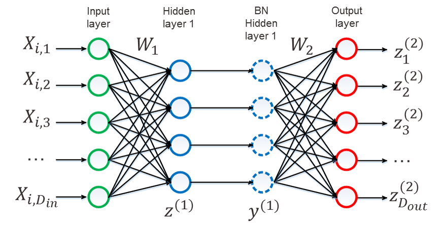 Figure 1
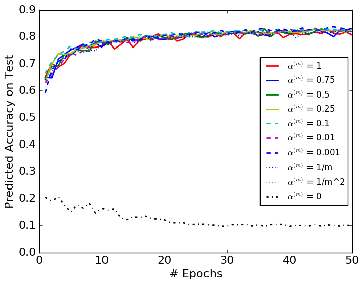 Figure 2
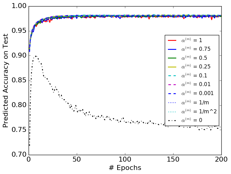 Figure 3
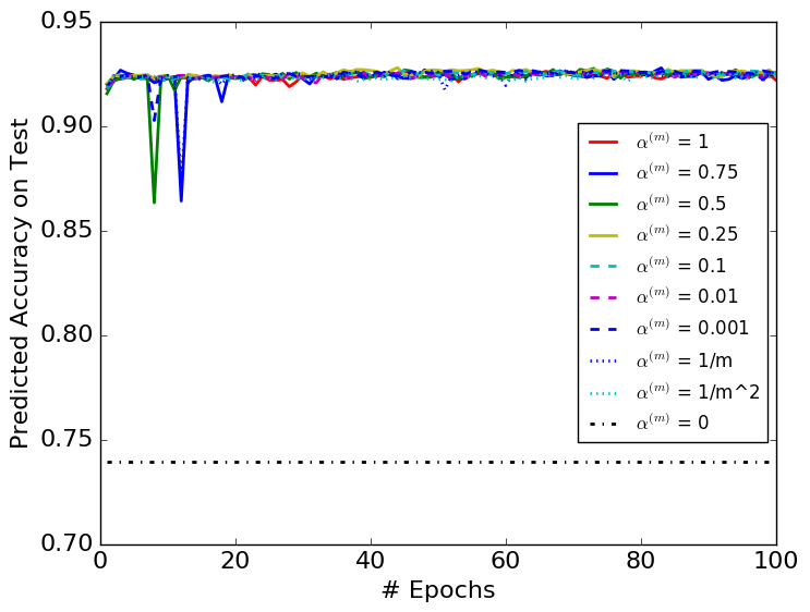 Figure 4
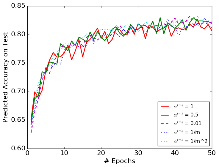 Figure 5
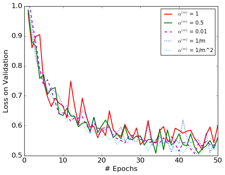 Figure 6
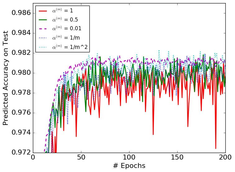 Figure 7
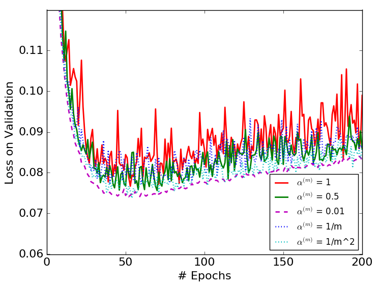 Figure 8
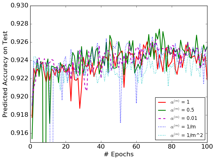 Figure 9
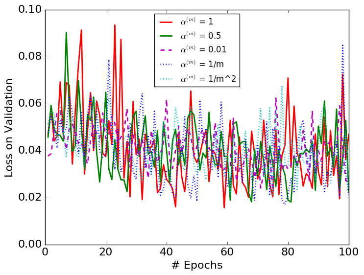 Figure 10
| Test Error | |||
|---|---|---|---|
| Model | MNIST | NI | CIFAR-10 |
| 2.70% | 7.69% | 17.31% | |
| 1.91% | 7.37% | 17.03% | |
| 1.84% | 7.46% | 17.11% | |
| 1.91% | 7.24% | 17.00% | |
| 1.90% | 7.36% | 17.10% | |
| 1.94% | 7.47% | 16.82% | |
| 1.95% | 7.43% | 16.28% | |
| 2.10% | 7.45% | 17.26% | |
| 2.00% | 7.59% | 17.23% | |
| 24.27% | 26.09% | 79.34% | |
Peer Reviews
No public reviews on file for this paper yet. If you reviewed it on a platform where reviews are public (OpenReview, ICLR, NeurIPS, ICML), you can paste yours below so the community can read it here.
Videos
No videos yet. Explain this paper in a talk, walkthrough, or lecture? Add one.
Taxonomy
TopicsAdvanced Neural Network Applications · Neural Networks and Applications · Stochastic Gradient Optimization Techniques
Methods*Communicated@Fast*How Do I Communicate to Expedia? · Batch Normalization
Diminishing Batch Normalization
\nameYintai Ma \[email protected]
\addrDepartment of Industrial Engineering
Northwestern University
Evanston, IL 60208, USA \AND\nameDiego Klabjan \[email protected]
\addrDepartment of Industrial Engineering & Management Science
Northwestern University
Evanston, IL 60208, USA
Abstract
In this paper, we propose a generalization of the Batch Normalization (BN) algorithm, diminishing batch normalization (DBN), where we update the BN parameters in a diminishing moving average way. BN is very effective in accelerating the convergence of a neural network training phase that it has become a common practice. Our proposed DBN algorithm remains the overall structure of the original BN algorithm while introduces a weighted averaging update to some trainable parameters. We provide an analysis of the convergence of the DBN algorithm that converges to a stationary point with respect to trainable parameters. Our analysis can be easily generalized for original BN algorithm by setting some parameters to constant. To the best knowledge of authors, this analysis is the first of its kind for convergence with Batch Normalization introduced. We analyze a two-layer model with arbitrary activation function. The convergence analysis applies to any activation function that satisfies our common assumptions. In the numerical experiments, we test the proposed algorithm on complex modern CNN models with stochastic gradients and ReLU activation. We observe that DBN outperforms the original BN algorithm on MNIST, NI and CIFAR-10 datasets with reasonable complex FNN and CNN models.
1 Introduction
Deep neural networks (DNN) have shown unprecedented success in various applications such as object detection. However, it still takes a long time to train a DNN until it converges. Ioffe and Szegedy (2015) identified a critical problem involved in training deep networks, internal covariate shift, and then proposed batch normalization (BN) to decrease this phenomenon. BN addresses this problem by normalizing the distribution of every hidden layer’s input. In order to do so, it calculates the pre-activation mean and standard deviation using mini-batch statistics at each iteration of training and uses these estimates to normalize the input to the next layer. The output of a layer is normalized by using the batch statistics, and two new trainable parameters per neuron are introduced that capture the inverse operation. It is now a standard practice Bottou et al. (2016); He et al. (2016). While this approach leads to a significant performance jump, to the best of our knowledge, there is no known theoretical guarantee for the convergence of an algorithm with BN. The difficulty of analyzing the convergence of the BN algorithm comes from the fact that not all of the BN parameters are updated by gradients. Thus, it invalidates most of the classical studies of convergence for gradient methods.
In this paper, we propose a generalization of the BN algorithm, diminishing batch normalization (DBN), where we update the BN parameters in a diminishing moving average way. It essentially means that the BN layer adjusts its output according to all past mini-batches instead of only the current one. It helps to reduce the problem of the original BN that the output of a BN layer on a particular training pattern depends on the other patterns in the current mini-batch, which is pointed out by Bottou et al. (2016). By setting the layer parameter we introduce into DBN to a specific value, we recover the original BN algorithm.
We give a convergence analysis of the algorithm with a two-layer batch-normalized neural network and diminishing stepsizes. We assume two layers (the generalization to multiple layers can be made by using the same approach but substantially complicating the notation) and an arbitrary loss function. The convergence analysis applies to any activation function that follows our common assumption. The main result shows that under diminishing stepsizes on gradient updates and updates on mini-batch statistics, and standard Lipschitz conditions on loss functions DBN converges to a stationary point. As already pointed out the primary challenge is the fact that some trainable parameters are updated by gradient while others are updated by a minor recalculation.
Contributions. The main contribution of this paper is in providing a general convergence guarantee for DBN. Specifically, we make the following contributions.
- •
In Section 4, we show conditions for the stepsizes and diminishing weights to ensure the convergence of BN parameters. The proof is provided in the appendix.
- •
We show that the algorithm converges to a stationary point under a general nonconvex objective function. To the best of our knowledge, this is the first convergence analysis that specifically considers transformations with BN layers.
This paper is organized as follows. In Section 2, we review the related works and the development of the BN algorithm. We formally state our model and algorithm in Section 3. We present our main results in Sections 4. In Section 5, we numerically show that the DBN algorithm outperforms the original BN algorithm. Proofs for main steps are collected in the Appendix.
2 Literature Review
Before the introduction of BN, it has long been known in the deep learning community that input whitening and decorrelation help to speed up the training process. In fact, Orr and Müller (2003) show that preprocessing the data by subtracting the mean, normalizing the variance, and decorrelating the input has various beneficial effects for back-propagation. Krizhevsky et al. (2012) propose a method called local response normalization which is inspired by computational neuroscience and acts as a form of lateral inhibition, i.e., the capacity of an excited neuron to reduce the activity of its neighbors. Gülçehre and Bengio (2016) propose a standardization layer that bears significant resemblance to batch normalization, except that the two methods are motivated by very different goals and perform different tasks.
Inspired by BN, several new works are taking BN as a basis for further improvements. Layer normalization Ba et al. (2016) is much like the BN except that it uses all of the summed inputs to compute the mean and variance instead of the mini-batch statistics. Besides, unlike BN, layer normalization performs precisely the same computation at training and test times. Normalization propagation that Arpit et al. (2016) uses data-independent estimations for the mean and standard deviation in every layer to reduce the internal covariate shift and make the estimation more accurate for the validation phase. Weight normalization also removes the dependencies between the examples in a minibatch so that it can be applied to recurrent models, reinforcement learning or generative models Salimans and Kingma (2016). Cooijmans et al. (2016) propose a new way to apply batch normalization to RNN and LSTM models. Recently, there are works on the insights and analysis of Batch Normalization. Bjorck et al. (2018) demonstrate how BN can help to correct training for ill-behaved normalized networks. Santurkar et al. (2018) claim that the key factor of BN is that it makes the optimization landscape much smoother and allows for faster training. However, these works do not cover a convergence analysis for BN and hence do not overlap with this work.
Given all these flavors, the original BN method is the most popular technique and for this reason our choice of the analysis. To the best of our knowledge, we are not aware of any prior analysis of BN.
BN has the gradient and non-gradient updates. Thus, nonconvex convergence results do not immediately transfer. Our analysis explicitly considers the workings of BN. However, nonconvex convergence proofs are relevant since some small portions of our analysis rely on known proofs and approaches.
Neural nets are not convex, even if the loss function is convex. For classical convergence results with a nonconvex objective function and diminishing learning rate, we refer to survey papers Bertsekas (2011); Bertsekas and Tsitsiklis (2000); Bottou et al. (2016). Bertsekas and Tsitsiklis (2000) provide a convergence result with the deterministic gradient with errors. Bottou et al. (2016) provide a convergence result with the stochastic gradient. The classic analyses showing the norm of gradients of the objective function going to zero date back to Grippo (1994); Polyak and Tsypkin (1973); Polyak (1987). For strongly convex objective functions with a diminishing learning rate, we learn the classic convergence results from Bottou et al. (2016).
3 Model and Algorithm
The optimization problem for a network is an objective function consisting of a large number of component functions, that reads:
[TABLE]
where , are real-valued functions for any data record . Index associates with data record and target response (hidden behind the dependency of on ) in the training set. Parameters include the common parameters updated by gradients directly associated with the loss function, while BN parameters are introduced by the BN algorithm and not updated by gradient methods but by mini-batch statistics. We define that the derivative of is always taken with respect to :
[TABLE]
The deep network we analyze has 2 fully-connected layers with neurons each. The techniques presented can be extended to more layers with additional notation. Each hidden layer computes with nonlinear activation function and is the input vector of the layer. We do not need to include an intercept term since the BN algorithm automatically adjusts for it. BN is applied to the output of the first hidden layer.
We next describe the computation in each layer to show how we obtain the output of the network. The notations introduced here is used in the analysis. Figure 1 shows the full structure of the network. The input data is vector , which is one of . Vector is the set of all BN parameters and vector is the set of all trainable parameters which are updated by gradients.
Matrices are the actual model parameters and are introduced by BN. The value of neuron of the first hidden layer is
[TABLE]
where denotes the weights of the linear transformations for the neuron.
The entry of batch-normalized output of the first layer is
[TABLE]
where and are trainable parameters updated by gradient and and are batch normalization parameters for . Trainable parameter is the mini-batch mean of and trainable parameter is the mini-batch sample deviation of . Constant keeps the denominator from zero. The output of entry of the output layer is:
[TABLE]
The objective function for the sample is
[TABLE]
where is the loss function associated with the target response . For sample , we have the following complete expression for the objective function:
[TABLE]
Function is nonconvex with respect to and .
3.1 Algorithm
Algorithm 1 shows the algorithm studied herein. There are two deviations from the standard BN algorithm, one of them actually being a generalization. We use the full gradient instead of the more popular stochastic gradient (SG) method. It essentially means that each batch contains the entire training set instead of a randomly chosen subset of the training set. An analysis of SG is potential future research. Although the primary motivation for full gradient update is to reduce the burdensome in showing the convergence, the full gradient method is similar to SG in the sense that both of them go through the entire training set, while full gradient goes through it deterministically and the SG goes through it in expectation. Therefore, it is reasonable to speculate that the SG method has similar convergence property as the full algorithm studied herein.
The second difference is that we update the BN parameters by their moving averages with respect to diminishing . The original BN algorithm can be recovered by setting for every . After introducing diminishing , and hence the output of the BN layer is determined by the history of all past data records, instead of those solely in the last batch. Thus, the output of the BN layer becomes more general that better reflects the distribution of the entire dataset. We use two strategies to decide the values of . One is to use a constant smaller than 1 for all , and the other one is to decay the gradually, such as .
In our numerical experiment, we show that Algorithm 1 outperforms the original BN algorithm, where both are based on SG and non-linear activation functions with many layers FNN and CNN models.
4 General Case
The main purpose of our work is to show that Algorithm 1 converges. In the general case, we focus on the nonconvex objective function.
4.1 Assumptions
Here are the assumptions we used for the convergence analysis.
Assumption 1
(Lipschitz continuity on and ).*
For every we have*
[TABLE]
[TABLE]
[TABLE]
Noted that the Lipschitz constants associated with each of the above inequalities are not necessarily the same. Here is an upper bound for these Lipschitz constants for simplicity.
Assumption 2
(bounded parameters).* There exists a constant such that weights and parameters are bounded element-wise by this constant in every iteration ,*
[TABLE]
Assumption 3
(diminishing update on ).* The stepsizes of update satisfy*
[TABLE]
This is a common assumption for diminishing stepsizes in optimization problems.
Assumption 4
(Lipschitz continuity of ).* Assume the loss functions for every is continuously differentiable. It implies that there exists such that*
[TABLE]
Assumption 5
(existence of a stationary point).* There exists a stationary point such that *
We note that all these are standard assumptions in convergence proofs. We also stress that Assumption 4 does not directly imply 1. Assumptions 1, 4 and 5 hold for many standard loss functions such as softmax and MSE.
Assumption 6
(Lipschitz at activation function).* The activation function is Lipschitz with constant :*
[TABLE]
Since for all activation function there is , the condition is equivalent to . We note that this assumption works for many popular choices of activation functions, such as ReLU and LeakyReLu.
4.2 Convergence Analysis
We first have the following lemma specifying sufficient conditions for to converge. Proofs for main steps are given in the Appendix.
Theorem 7
Under Assumptions 1, 2, 3 and 6, if satisfies
[TABLE]
then sequence converges to .
We show in Theorem 11 that this converges to , where the loss function reaches zero gradients, i.e., is a stationary point. We give a discussion of the above conditions for and at the end of this section. With the help of Theorem 7, we can show the following convergence result.
Lemma 8
Under Assumptions 4, 5 and the assumptions of Theorem 7, when
[TABLE]
we have
[TABLE]
This result is similar to the classical convergence rate analysis for the non-convex objective function with diminishing stepsizes, which can be found in Bottou et al. (2016).
Lemma 9
Under the assumptions of Lemma 8, we have
[TABLE]
This theorem states that for the full gradient method with diminishing stepsizes the gradient norms cannot stay bounded away from zero. The following result characterizes more precisely the convergence property of Algorithm 1.
Lemma 10
Under the assumptions stated in Lemma 8, we have
[TABLE]
Our main result is listed next.
Theorem 11
Under the assumptions stated in Lemma 8, we have
[TABLE]
It shows that the DBN algorithm converges to a stationary point where the norm of gradient is zero. We cannot show that ’s converges (standard convergence proofs are also unable to show such a stronger statement). For this reason, Theorem 11 does not immediately follow from Lemma 10 together with Theorem 7. The statement of Theorem 11 would easily follow from Lemma 10 if the convergence of is established and the gradient being continuous.
Considering the cases and . We show in the appendix that the set of sufficient and necessary conditions to satisfy the assumptions of Theorem 7 are and . The set of sufficient and necessary conditions to satisfy the assumptions of Lemma 8 are and . For example, we can pick and to achieve the above convergence result in Theorem 11.
5 Computational Experiments
We conduct the computational experiments with Theano and Lasagne on a Linux server with a Nvidia Titan-X GPU. We use MNIST LeCun et al. (1998), CIFAR-10 Krizhevsky and Hinton (2009) and Network Intrusion (NI) kdd (1999) datasets to compare the performance between DBN and the original BN algorithm. For the MNIST dataset, we use a four-layer fully connected FNN () with the ReLU activation function and for the NI dataset, we use a four-layer fully connected FNN () with the ReLU activation function. For the CIFAR-10 dataset, we use a reasonably complex CNN network that has a structure of (Conv-Conv-MaxPool-Dropout-Conv-Conv-MaxPool-Dropout-FC-Dropout-FC), where all four convolution layers and the first fully connected layers are batch normalized. We use the softmax loss function and regularization with for all three models. All the trainable parameters are randomly initialized before training. For all 3 datasets, we use the standard epoch/minibatch setting with the minibatch size of , i.e., we do not compute the full gradient and the statistics are over the minibatch. We use AdaGrad Duchi, John and Hazan, Elad and Singer (2011) to update the learning rates for trainable parameters, starting from .
We use two different strategies to decide the values of in DBN: constant values of and diminishing where and . We test the choices of constant .
We test all the choices of with the performances presented in Figure 2. Figure 2 shows that all the non-zero choices of converge properly. The algorithms converge without much difference even when in DBN is very small, e.g., . However, if we select , the algorithm is erratic. Besides, we observe that all the non-zero choices of converge at a similar rate. The fact that DBN keeps the batch normalization layer stable with a very small suggests that the BN parameters do not have to be depended on the latest minibatch, i.e., the original BN.
We compare a selected set of the most efficient choices of in Figures 3 and 4. They show that DBN with is more stable than the original BN algorithm. The variances with respect to epochs of the DBN algorithm are smaller than those of the original BN algorithms in each figure.
Table 1 shows the best result obtained from each choice of . Most importantly, it suggests that the choices of and perform better than the original BN algorithm. Besides, all the constant less-than-one choices of perform better than the original BN, showing the importance of considering the mini-batch history for the update of the BN parameters. The BN algorithm in each figure converges to similar error rates on test datasets with different choices of except for the case. Among all the models we tested, is the only one that performs top 3 for all three datasets, thus the most robust choice.
To summarize, our numerical experiments show that the DBN algorithm outperforms the original BN algorithm on the MNIST, NI and CIFAT-10 datasets with typical deep FNN and CNN models.
**Future Directions. ** On the analytical side, we believe an extension to more than 2 layers is doable with significant augmentations of the notation. A stochastic gradient version is likely to be much more challenging to analyze. A second open question concerns analyzing the algorithm with a mini-batch setting. We believe it can be done by reusing most of the present analysis and changing some of the notation for wrapped layers.
Appendix A: Proofs.
Preliminary Results
Proposition 12
There exists a constant M such that, for any in iteration and fixed , we have
[TABLE]
Proof. By Assumption 5, we know there exists such that . Then we have
[TABLE]
where the last inequality is by Assumption 1. We then have
[TABLE]
because are bounded by Assumption 2.
Proposition 13
We have
[TABLE]
Proof. This is a known result of the Lipschitz-continuous condition that can be found in Bottou et al. (2016). We have this result together with Assumption 1.
Proof of Theorem 7
Lemma 14
*When ,
is a Cauchy series.*
Proof. By Algorithm 1, we have
[TABLE]
We define and . After dividing (21) by , we obtain
[TABLE]
Then we have
[TABLE]
[TABLE]
[TABLE]
[TABLE]
[TABLE]
[TABLE]
[TABLE]
Equation (Proof of Theorem 7) is due to
Therefore,
[TABLE]
It remains to show that
[TABLE]
[TABLE]
implies the convergence of . By (28), we have since
It is also easy to show that there exists and such that for all , we have
[TABLE]
Therefore,
Thus the following holds:
[TABLE]
and
[TABLE]
From (29) and (32) it follows that the sequence is a Cauchy series.
Lemma 15
Since is a Cauchy series, is a Cauchy series.
Proof. We know that Since and we have Thus is a Cauchy series.
Lemma 16
If , is a Cauchy series.
Proof. We define . Then we have
[TABLE]
[TABLE]
Since is convergent, there exists , and such that for any , . For any \bar{C}\in\left\{\dfrac{c_{1}}{{\color[rgb]{0,0,0}k}},\dfrac{c_{2}}{{\color[rgb]{0,0,0}k}}\right\}, we have
[TABLE]
[TABLE]
[TABLE]
[TABLE]
[TABLE]
Inequality (35) is by the following fact:
[TABLE]
where and for every are arbitrary real scalars. Besides, (39) is due to
Inequality (36) follow from the square function being increasing for nonnegative numbers. Besides these facts, (36) is also by the same techniques we used in (23)-(25) where we bound the derivatives with the Lipschitz continuity in the following inequality:
[TABLE]
Inequality (37) is by collecting the bounded terms into a single bound . Therefore,
[TABLE]
Using the similar methods in deriving (28) and (29), it can be seen that a set of sufficient conditions ensuring the convergence for is: and
Therefore, the convergence conditions for are the same as for .
It is clear that these lemmas establish the proof of Theorem 7.
Consequences of Theorem 7
Proposition 17
Under the assumptions of Theorem 7, we have where
[TABLE]
* and are constants. *
Proof. For the upper bound of , by (38), we have
[TABLE]
We define . Therefore,
[TABLE]
The first inequality comes by substituting by and by taking as in (41). The second inequality comes from (30). We then obtain,
[TABLE]
The second inequality is by , the third inequality is by (30) and the last inequality can be easily seen by induction. By (44), we obtain
[TABLE]
Therefore, we have
[TABLE]
The first inequality is by (45), the second inequality is by (41), the third inequality is by (31) and the fourth inequality is by adding the nonnegative term to the right-hand side.
For the upper bound of we have
[TABLE]
Let us define and . Recall from Theorem 7 that is a Cauchy series, by (27), Therefore, the first term in (47) is bounded by
[TABLE]
For the second term in (47), recall that . Then we have where the inequality can be easily seen by induction. Therefore, the second term in (47) is bounded by
[TABLE]
From these we obtain
[TABLE]
The first inequality is by (47) and the second inequality is by (48) and (49). Combining (46) and (50), we have that
[TABLE]
where and are constants defined as M_{1}=\max(\dfrac{\tilde{M}_{\bar{L},M}|{\color[rgb]{0,0,0}k}|}{C},\bar{M}_{\bar{L},M}) and M_{2}=\max(\dfrac{\bar{\sigma}_{j}+|{\color[rgb]{0,0,0}k}||\bar{C}|}{C},\dfrac{\bar{\mu}_{j}}{C}).\hfill\Box
Proposition 18
Under the assumptions of Theorem 7,
[TABLE]
where is defined in Proposition 17.
Proof. For simplicity of the proof, let us define
We have
[TABLE]
where is the dimension of . The second inequality is by Assumption 1 and the fourth inequality is by Proposition 17. Inequality (51) implies that for all and , we have
It remains to show
[TABLE]
This is established by the following four cases.
-
If , then . Thus by Proposition 12.
-
If , then , and
-
If , then , and
-
If , then , and . The last inequality is by Proposition 12.
All these four cases yield (52).
Proposition 19
Under the assumptions of Theorem 7, we have
[TABLE]
where is a constant and is defined in Proposition 17.
Proof. By Proposition 13,
[TABLE]
Therefore, we can sum it over the entire training set from to to obtain
[TABLE]
In Algorithm 1, we define the update of in the following full gradient way:
[TABLE]
which implies
[TABLE]
By (56) we have We now substitute , and into (54) to obtain
[TABLE]
The first inequality is by plugging (56) into (54), the second inequality comes from Proposition 12 and the third inequality comes from Proposition 18.
Proof of Theorem 11
Here we show Theorem 11 as the consequence of Theorem 7 and Lemmas 8, 9 and 10.
Proof of Lemma 8
Here we show Lemma 8 as the consequence of Lemmas 20, 21 and 22.
Lemma 20
* and is a set of sufficient condition to ensure*
[TABLE]
Proof. By plugging (45) and (43) into (58), we have the following for all :
[TABLE]
It is easy to see that the the following conditions are sufficient for right-hand side of (59) to be finite: and
Therefore, we obtain
Lemma 21
Under Assumption 4,
[TABLE]
is a set of sufficient conditions to ensure
[TABLE]
Proof. By Assumption 4, we have
[TABLE]
By the definition of , we then have
[TABLE]
The first inequality is by the Cauchy-Schwarz inequality, and the second one is by (60). To show the finiteness of (64), we only need to show the following two statements:
[TABLE]
and
[TABLE]
Proof of (65): For all we have
[TABLE]
The inequality comes from , where is the dimension of and is the element-wise upper bound for in Assumption 2.
Finally, we invoke Lemma 14 to assert that is finite.
Proof of (66): For all we have
[TABLE]
The first term in (68) is finite since is a Cauchy series. For the second term, we know that there exists a constant such that for all , This is also by the fact that is a Cauchy series and it converges to . Therefore, the second term in (68) becomes
[TABLE]
Noted that function is Lipschitz continuous since its gradient is bounded by . Therefore we can choose as the Lipschitz constant for . We then have the following inequality:
[TABLE]
Plugging (70) into (69), we obtain
[TABLE]
where the first term is finite by the fact that is a finite constant. We have shown the condition for the second term to be finite in Lemma 20. Therefore,
[TABLE]
By (65) and (66), we have that the right-hand side of (64) is finite. It means that the left-hand side of (64) is finite. Thus,
Lemma 22
If
[TABLE]
then
[TABLE]
Proof. For simplicity of the proof, we define
[TABLE]
[TABLE]
[TABLE]
[TABLE]
where is the converged value of in Theorem 7. Therefore,
[TABLE]
By Proposition 19,
[TABLE]
We sum the inequality (72) from 1 to with respect to and plug (73) into it to obtain
[TABLE]
From this, we have:
[TABLE]
Next we show that each of the four terms in the right-hand side of (75) is finite, respectively. For the first term,
[TABLE]
is by the fact that the parameters are bounded by Assumption 2, which implies that the image of is in a bounded set.
For the second term, we showed its finiteness in Lemma 21.
For the third term, by (42), we have
[TABLE]
The right-hand side of (77) is finite because
[TABLE]
and
[TABLE]
The second inequalities in (78) and (79) come from the stated assumptions of this lemma.
For the fourth term,
[TABLE]
holds, because we have in Assumption 3. Therefore, holds.
In Lemmas 20, 21 and 22, we show that and are Cauchy series, hence Lemma 8 holds.
Proof of Lemma 9
This proof is similar to the the proof by Bertsekas and Tsitsiklis (2000).
Proof. By Theorem 8, we have
[TABLE]
If there exists a and an integer such that
[TABLE]
for all , we would have
[TABLE]
which contradicts (81). Therefore,
Proof of Lemma 10
Lemma 23
Let and be three sequences such that is nonnegative for all . Assume that
[TABLE]
and that the series converges as . Then either or else converges to a finite value and .
This lemma has been proven by Bertsekas and Tsitsiklis (2000).
Lemma 24
When
[TABLE]
it follows that converge to a finite value.
Proof. By Proposition 19, we have
[TABLE]
Let , and . By (10) and (77)- (79), it is easy to see that converges as . Therefore, by Lemma 23, converges to a finite value. The infinite case can not occur in our setting due to Assumptions 1 and 2.
Lemma 25
If
**
then .
Proof. To show that , assume the contrary; that is,
[TABLE]
Then there exists an such that for infinitely many and also for infinitely many . Therefore, there is an infinite subset of integers , such that for each , there exists an integer such that
[TABLE]
From it follows that for all that are sufficiently large so that , we have
[TABLE]
Otherwise the condition would be violated. Without loss of generality, we assume that the above relations as well as (57) hold for all . With the above observations, we have for all ,
[TABLE]
The first inequality is by (86) and the third one is by the Lipschitz condition assumption. The seventh one is by (51). By (12), we have for all ,
[TABLE]
and
[TABLE]
It is easy to see that for any sequence with , if follows that . Therefore, and From this it follows that
[TABLE]
By (51) and (87), if we pick such that , we have Using (57), we observe that
[TABLE]
where the second inequality is by (87). By Lemma 24, and converge to the same finite value. Using this convergence result and the assumption , this relation implies that
and contradicts (91).
By Lemmas 23, 24 and 25, we show that Theorem 11 holds.
Discussions of conditions for stepsizes
Here we discuss the actual conditions for and to satisfy the assumptions of Theorem 7 and Lemma 8. We only consider the cases and , but the same analysis applies to the cases and .
Assumptions of Theorem 7
For the assumptions of Theorem 7, the first condition requires . Besides, the second condition
[TABLE]
requires . The approximation comes from the fact that for every we have
[TABLE]
Since due to Assumption 3, we conclude that Therefore, the conditions for and to satisfy the assumptions of Theorem 7 are and .
Assumptions of Lemma 8
For the assumptions of Theorem 7, the first condition
[TABLE]
requires .
Besides, the second condition is
[TABLE]
The inequality holds because for any , we have
[TABLE]
Therefore, the conditions for and to satisfy the assumptions of Lemma 8 are and .
The reference list from the paper itself. Each links out to its DOI / PubMed record.
- 1kdd (1999) KDD Cup 1999 Data, 1999. URL http://www.kdd.org/kdd-cup/view/kdd-cup-1999/Data .
- 2Arpit et al. (2016) Devansh Arpit, Yingbo Zhou, Bhargava U. Kota, and Venu Govindaraju. Normalization Propagation: A Parametric Technique for Removing Internal Covariate Shift in Deep Networks. In International Conference on Machine Learning , volume 48, page 11, 2016.
- 3Ba et al. (2016) Jimmy Lei Ba, Jamie Ryan Kiros, and Geoffrey E. Hinton. Layer Normalization. ar Xiv preprint ar Xiv:1607.06450 , 2016.
- 4Bertsekas (2011) Dimitri P. Bertsekas. Incremental gradient, subgradient, and proximal methods for convex optimization: A Survey. Optimization for Machine Learning , 2010(3):1–38, 2011.
- 5Bertsekas and Tsitsiklis (2000) Dimitri P. Bertsekas and John N. Tsitsiklis. Gradient Convergence in Gradient Methods with Errors. SIAM Journal on Optimization , 10:627–642, 2000.
- 6Bjorck et al. (2018) Johan Bjorck, Carla Gomes, Bart Selman, and Kilian Q. Weinberger. Understanding batch normalization. ar Xiv preprint ar Xiv:1806.02375 , 2018.
- 7Bottou et al. (2016) Léon Bottou, Frank E. Curtis, and Jorge Nocedal. Optimization Methods for Large-Scale Machine Learning. ar Xiv preprint ar Xiv:1606.04838 , 2016.
- 8Cooijmans et al. (2016) Tim Cooijmans, Nicolas Ballas, César Laurent, and Aaron Courville. Recurrent Batch Normalization. ar Xiv preprint ar Xiv:1603.09025 , 2016.