Liquid Cloud Storage
Michael G. Luby, Roberto Padovani, Thomas J. Richardson, Lorenz, Minder, Pooja Aggarwal

TL;DR
Liquid cloud storage systems distribute data redundantly across many unreliable nodes, using advanced coding and repair strategies to optimize durability, overhead, bandwidth, and performance.
Contribution
This paper introduces a liquid storage architecture that combines large coding, lazy repair, and flow organization to optimize multiple storage metrics.
Findings
Liquid systems can achieve flexible, near-optimal trade-offs among durability, overhead, and repair bandwidth.
The proposed design enables scalable and reliable object storage across large, unreliable networks.
The system's strategies improve efficiency and resilience compared to traditional storage methods.
Abstract
A liquid system provides durable object storage based on spreading redundantly generated data across a network of hundreds to thousands of potentially unreliable storage nodes. A liquid system uses a combination of a large code, lazy repair, and a flow storage organization. We show that a liquid system can be operated to enable flexible and essentially optimal combinations of storage durability, storage overhead, repair bandwidth usage, and access performance.
Click any figure to enlarge with its caption.
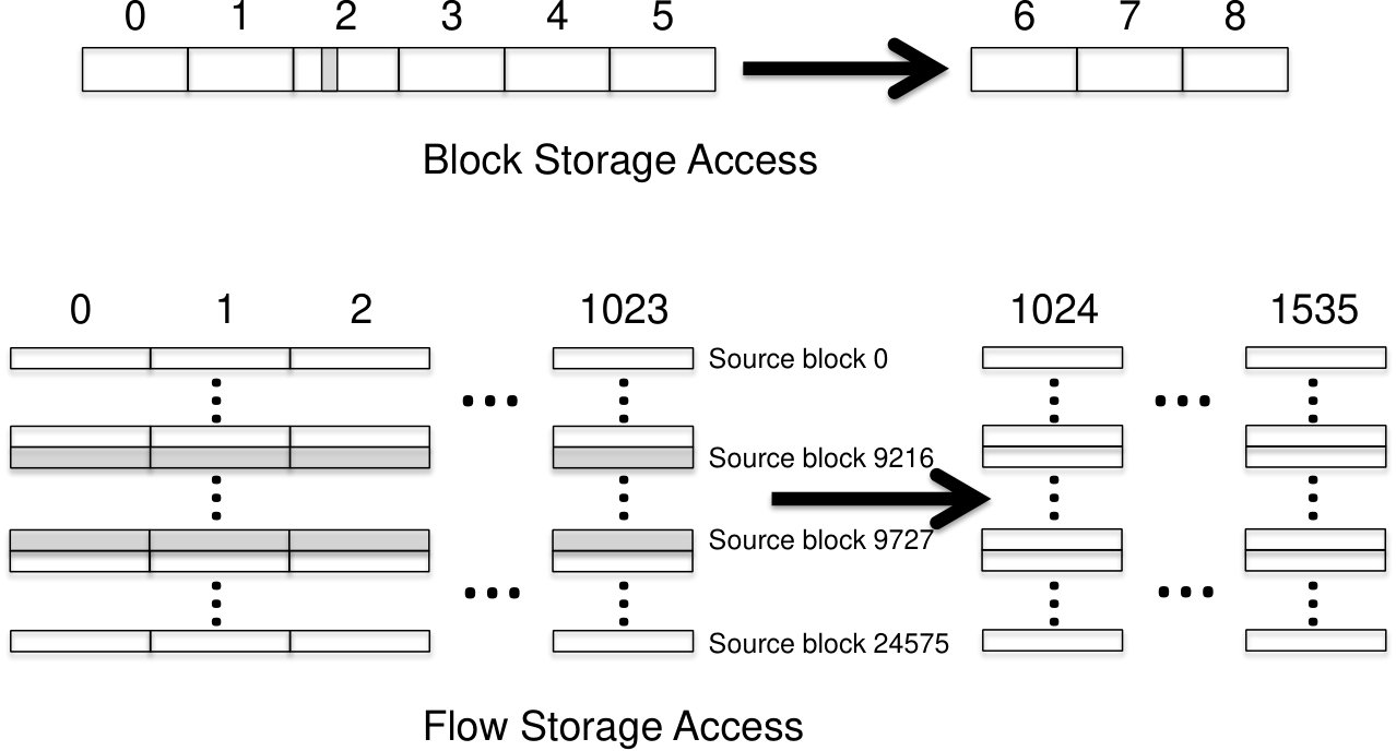 Figure 1
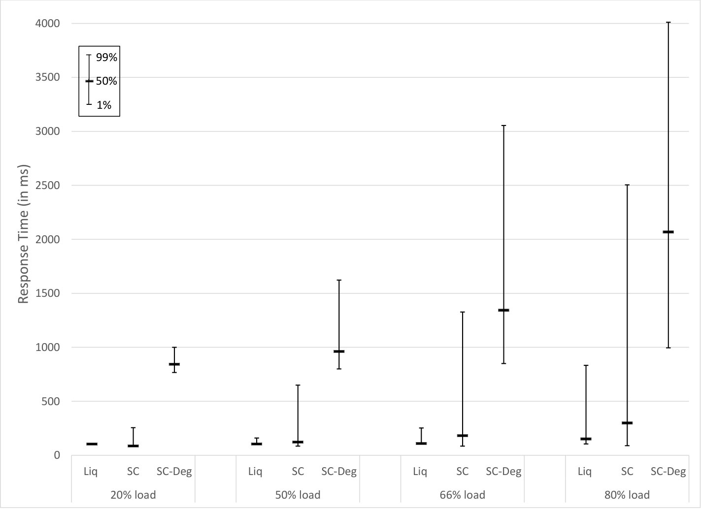 Figure 2
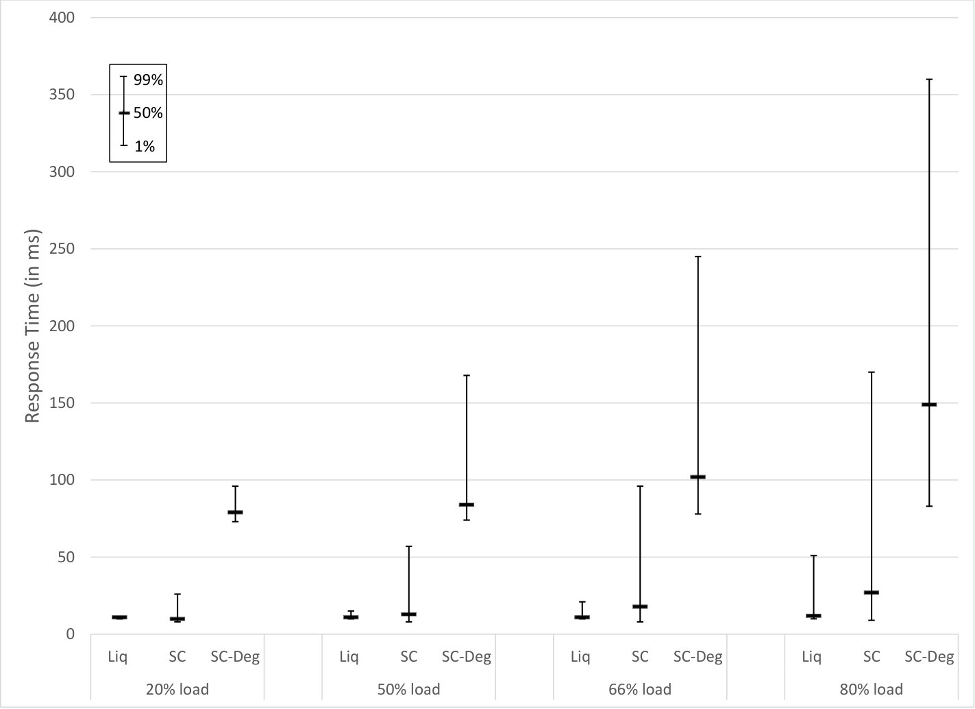 Figure 3
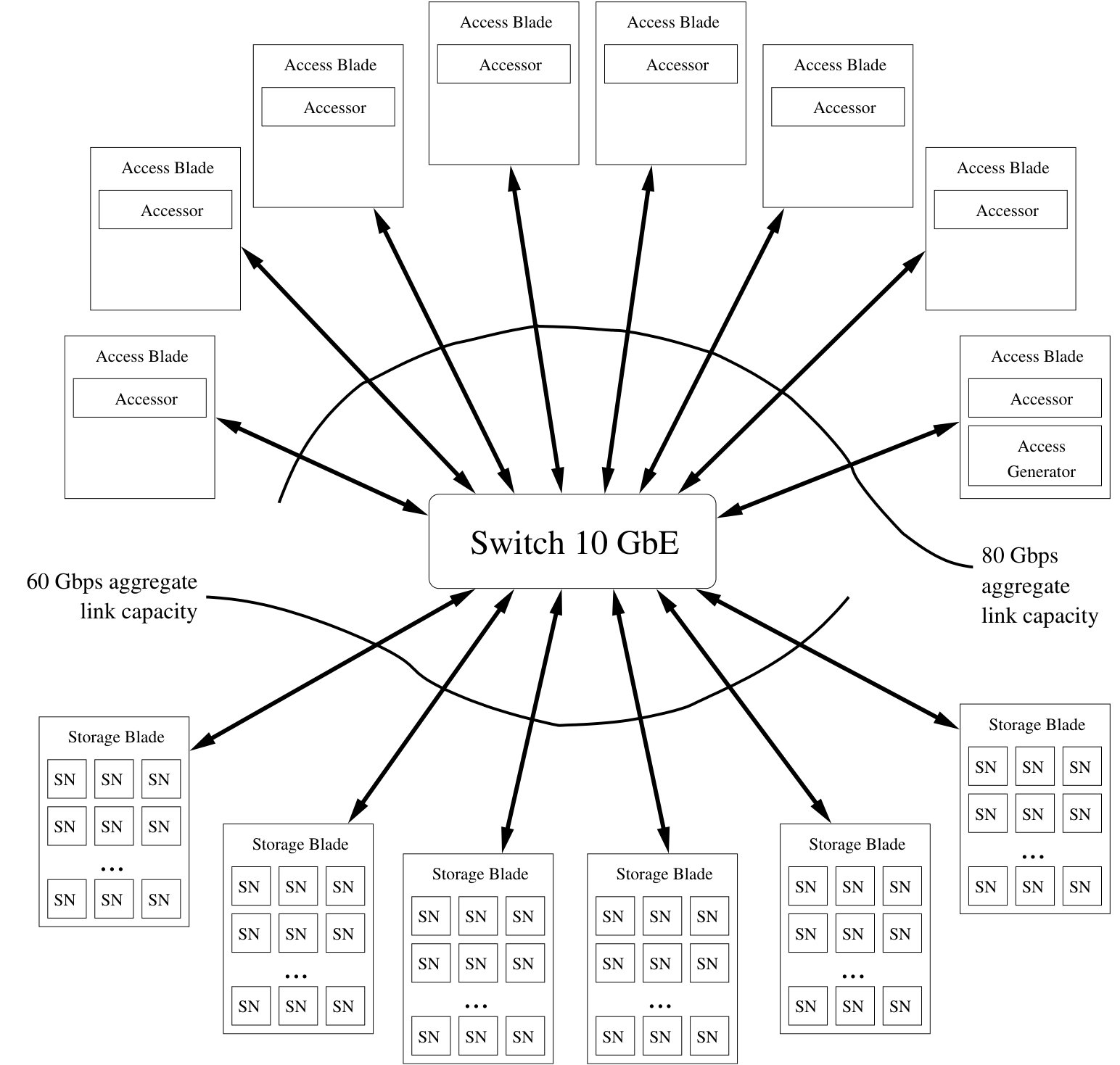 Figure 4
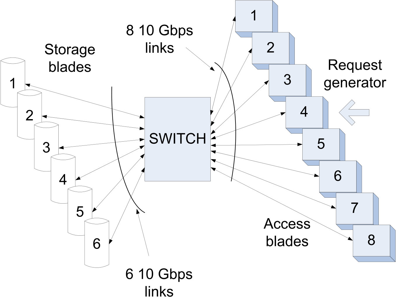 Figure 5
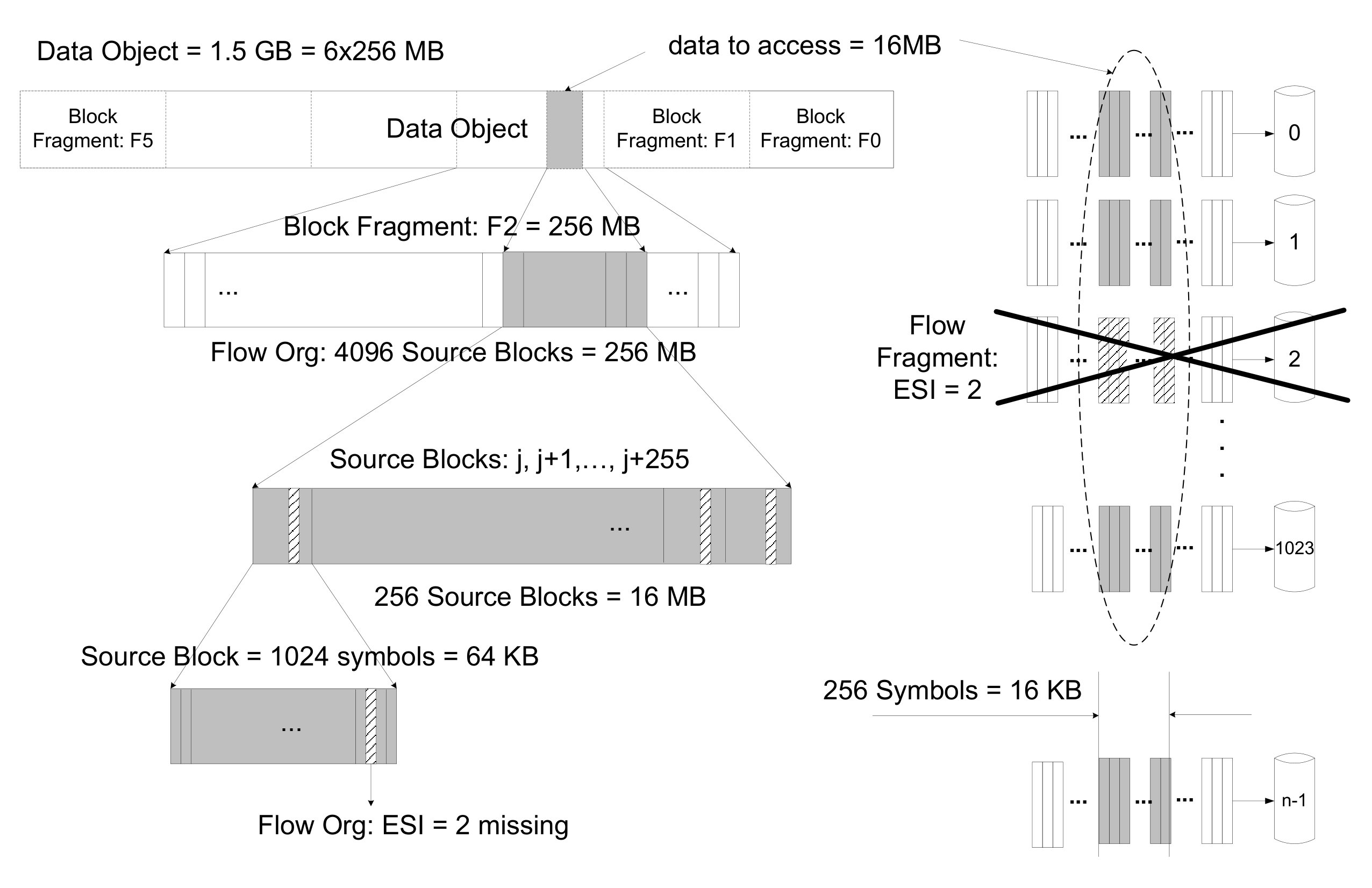 Figure 6
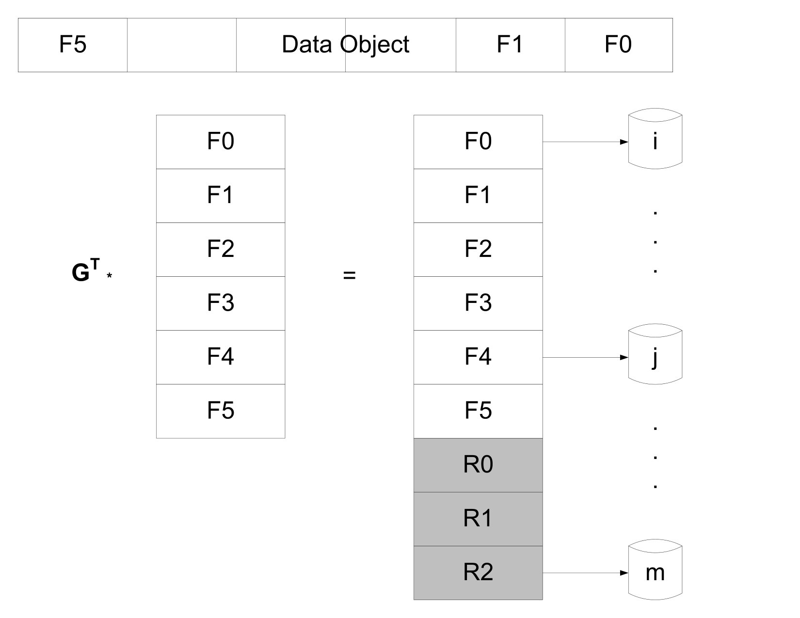 Figure 7
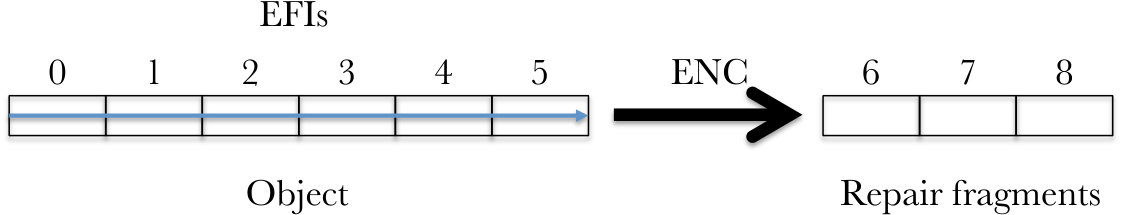 Figure 8
 Figure 9
 Figure 10
 Figure 11
 Figure 12
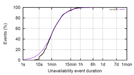 Figure 13
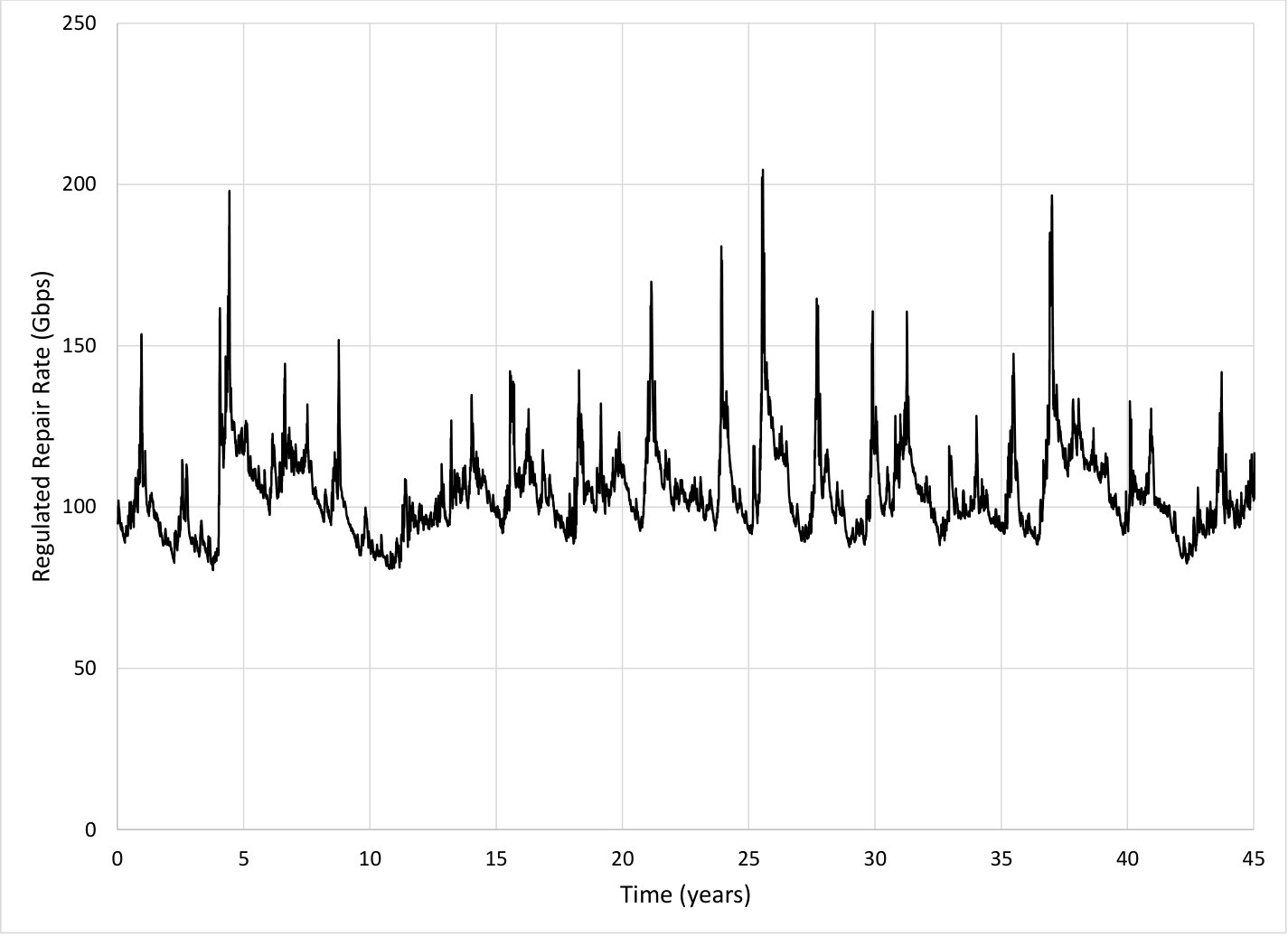 Figure 14
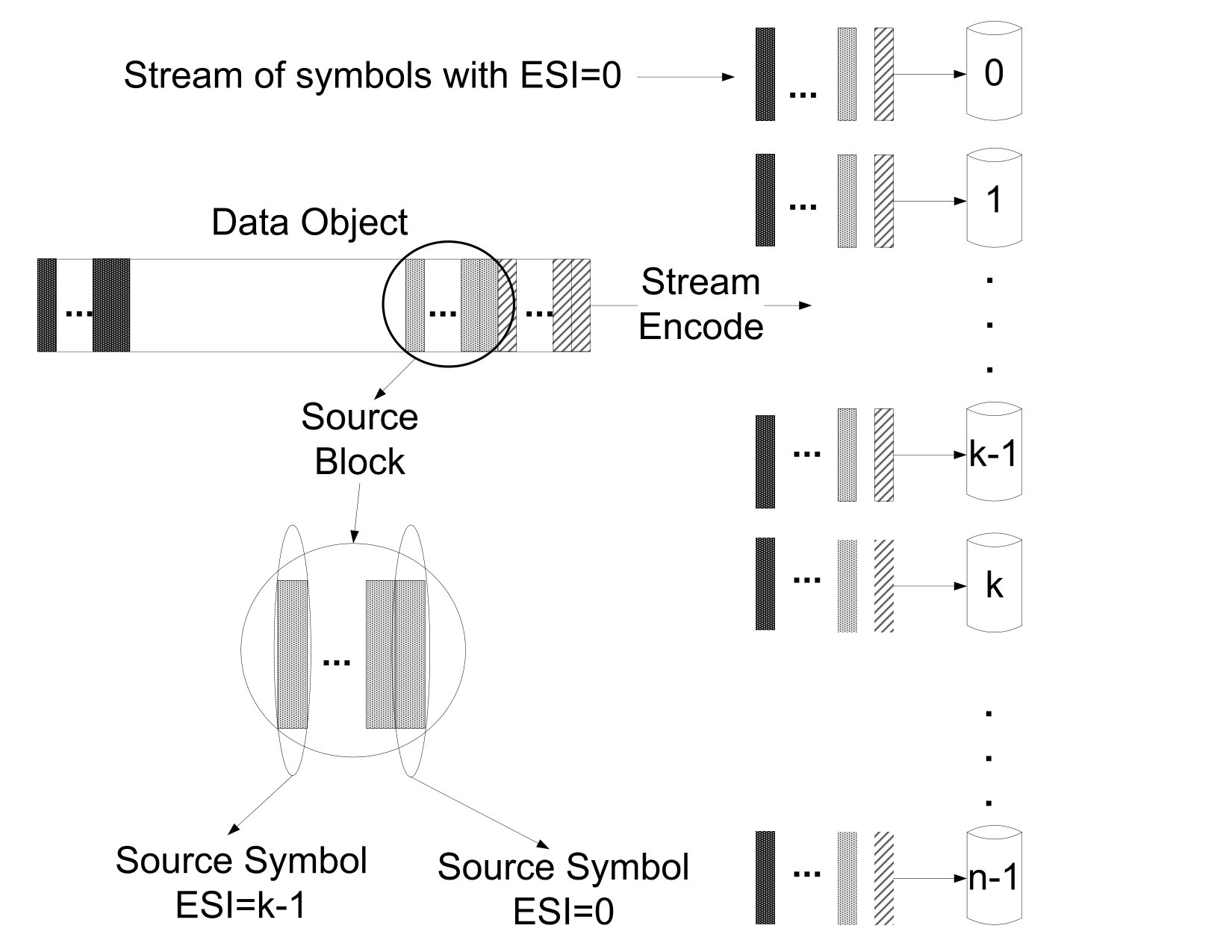 Figure 15
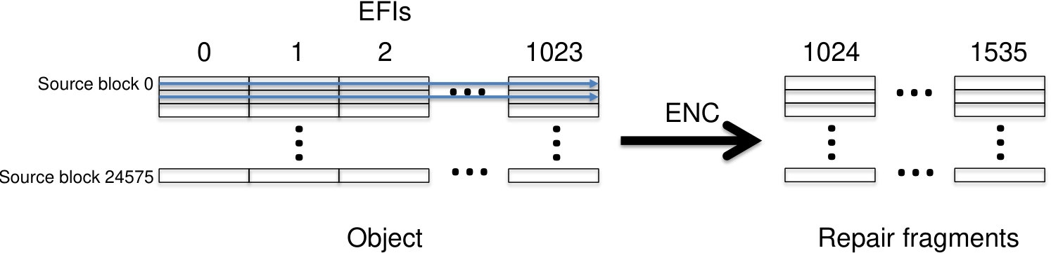 Figure 16
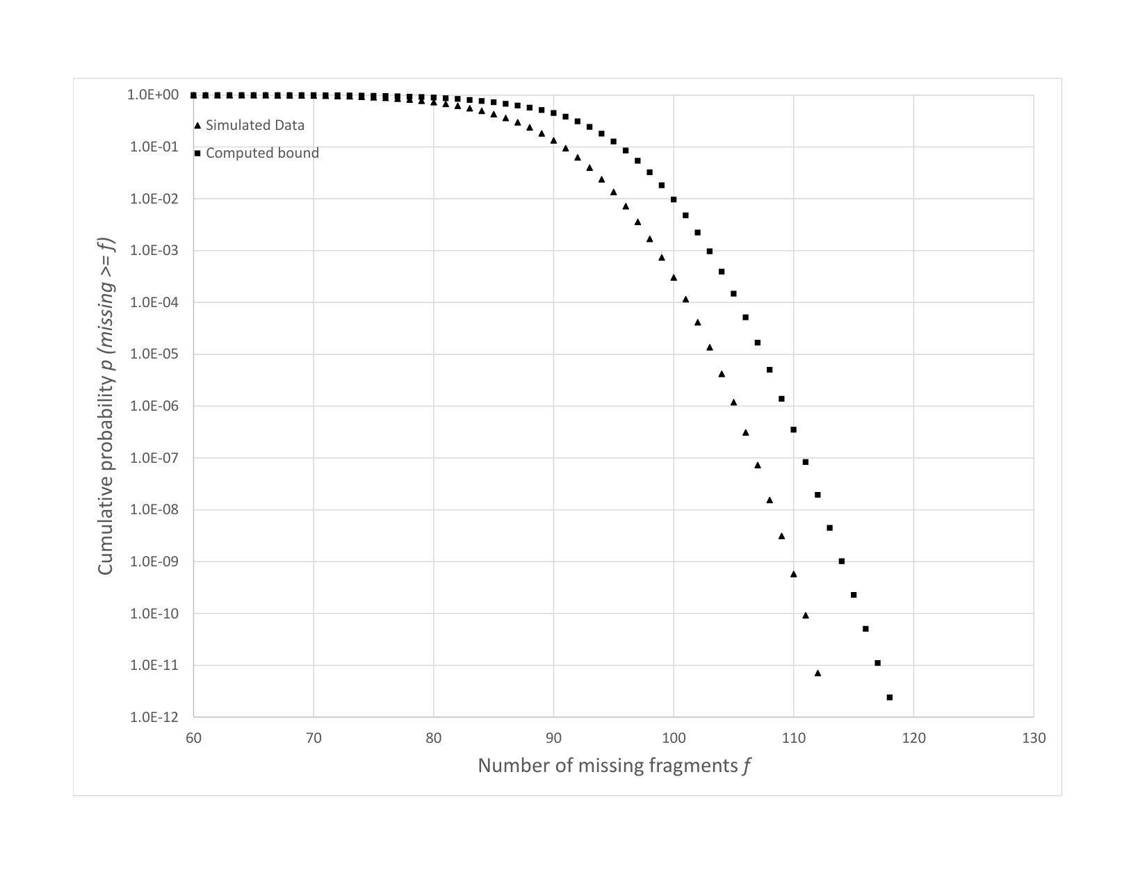 Figure 17
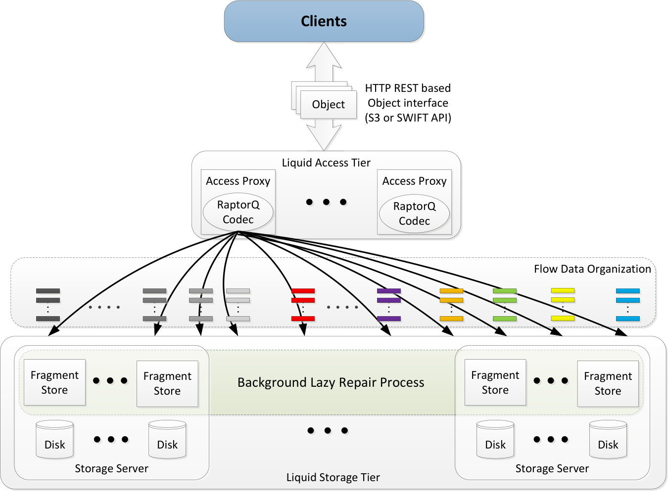 Figure 18
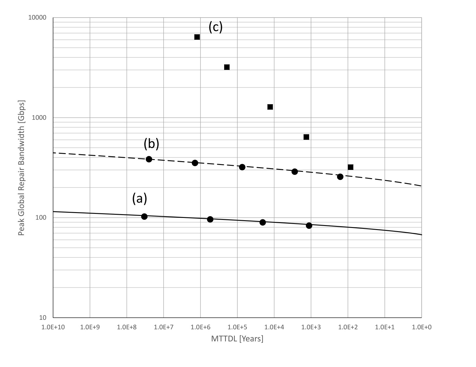 Figure 19
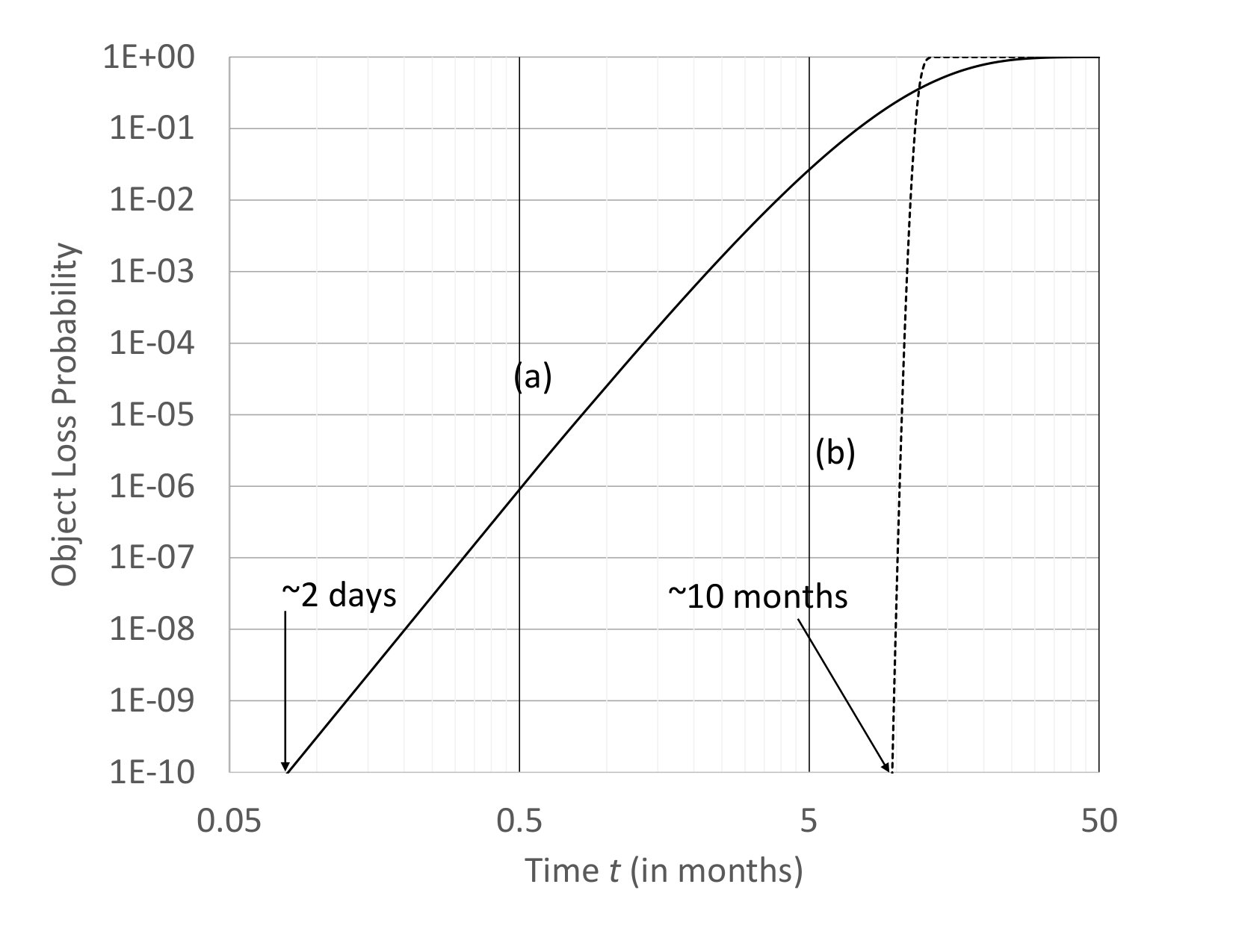 Figure 20
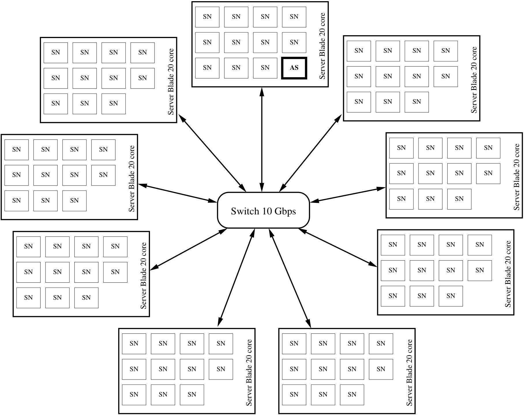 Figure 21
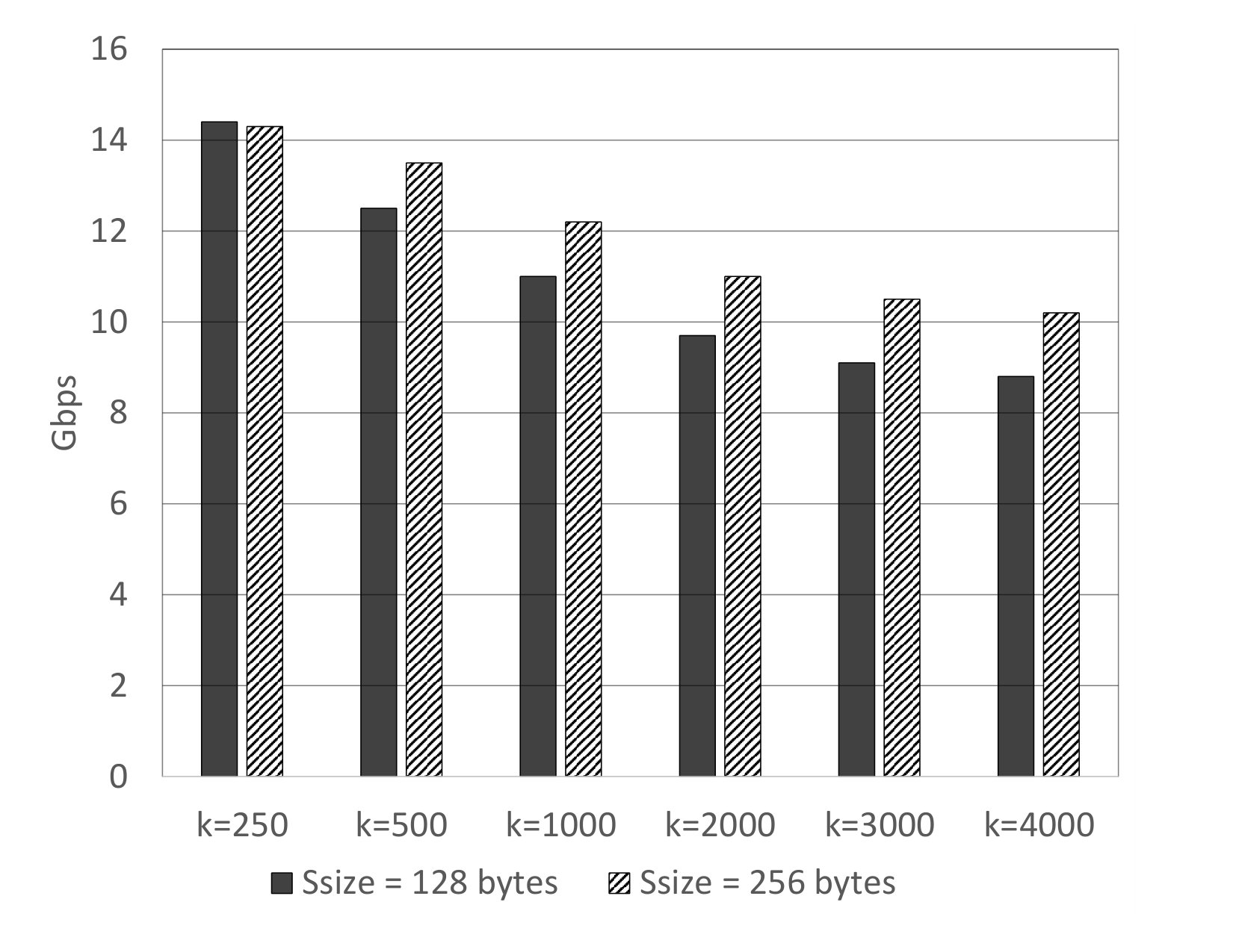 Figure 22
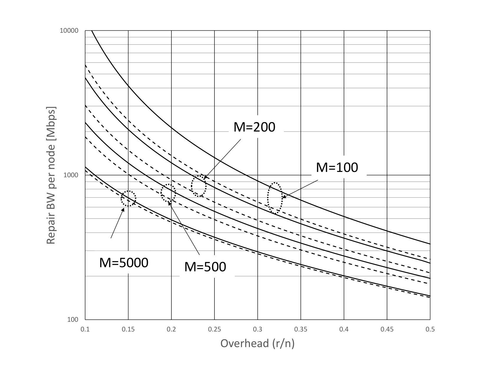 Figure 23
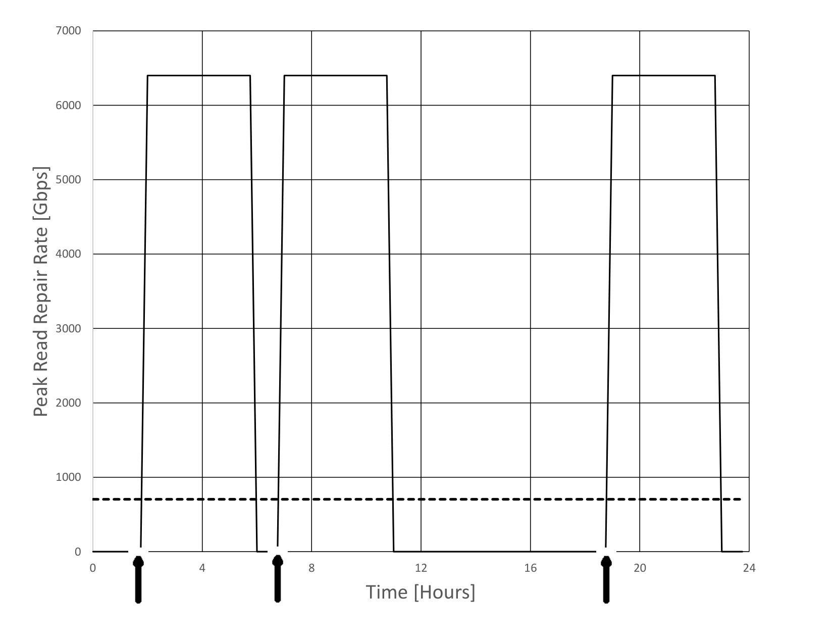 Figure 24
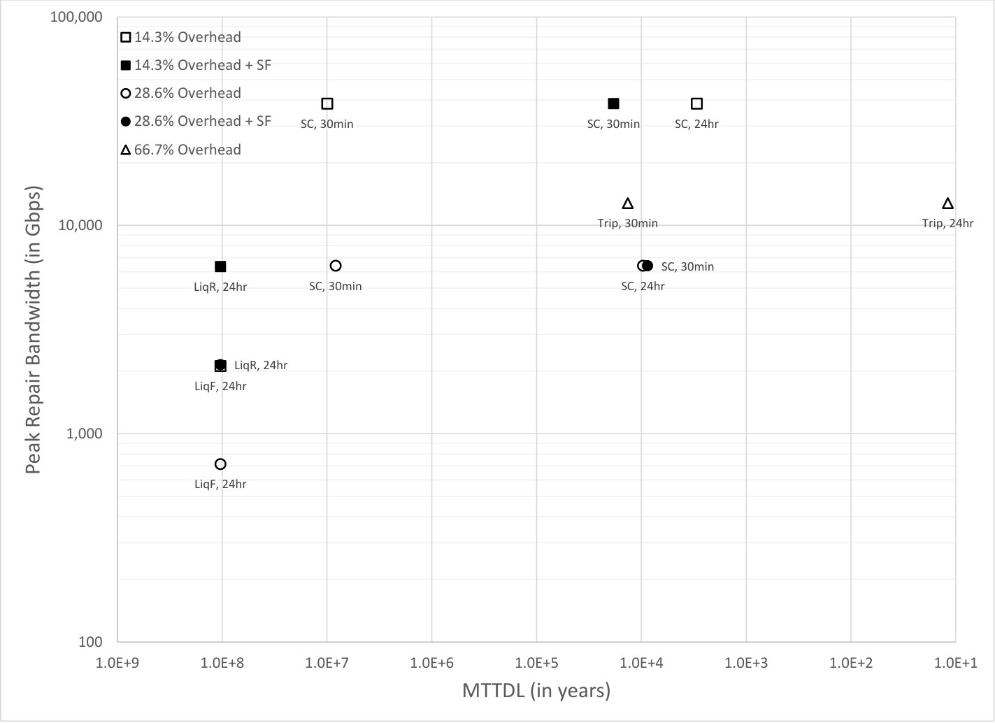 Figure 25
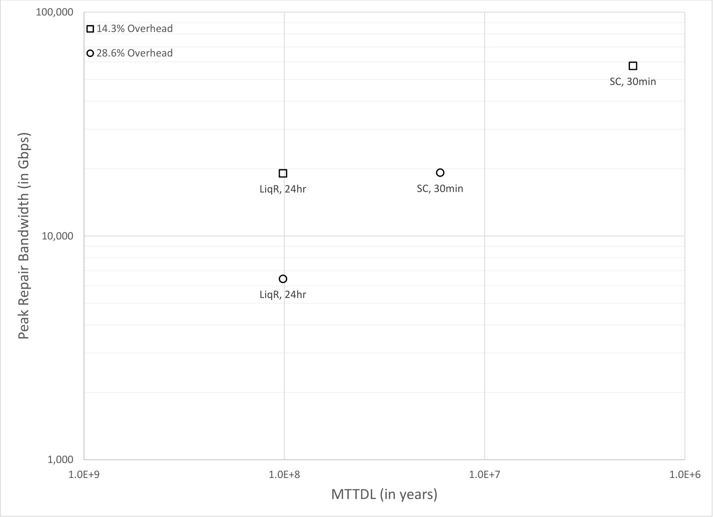 Figure 26
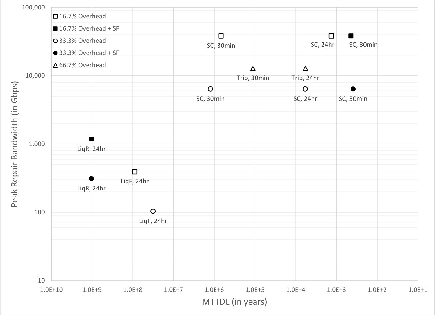 Figure 27
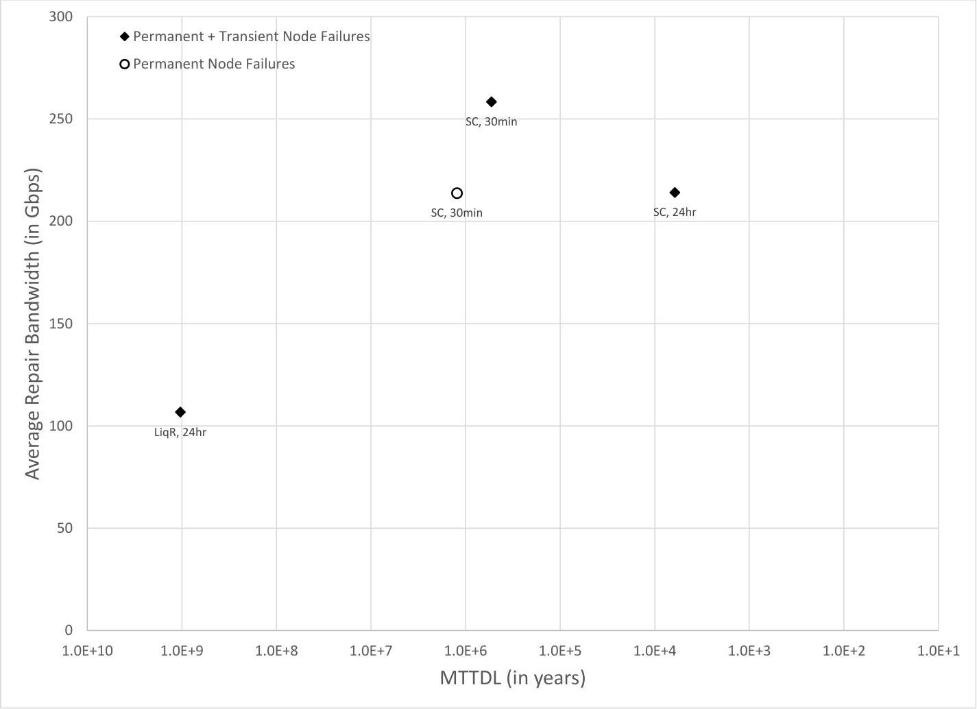 Figure 28
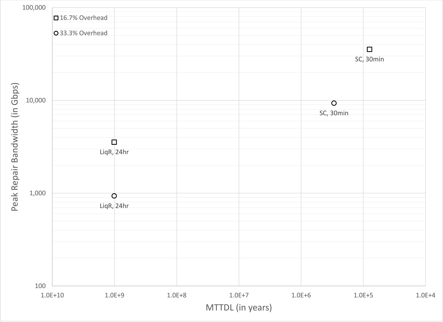 Figure 29
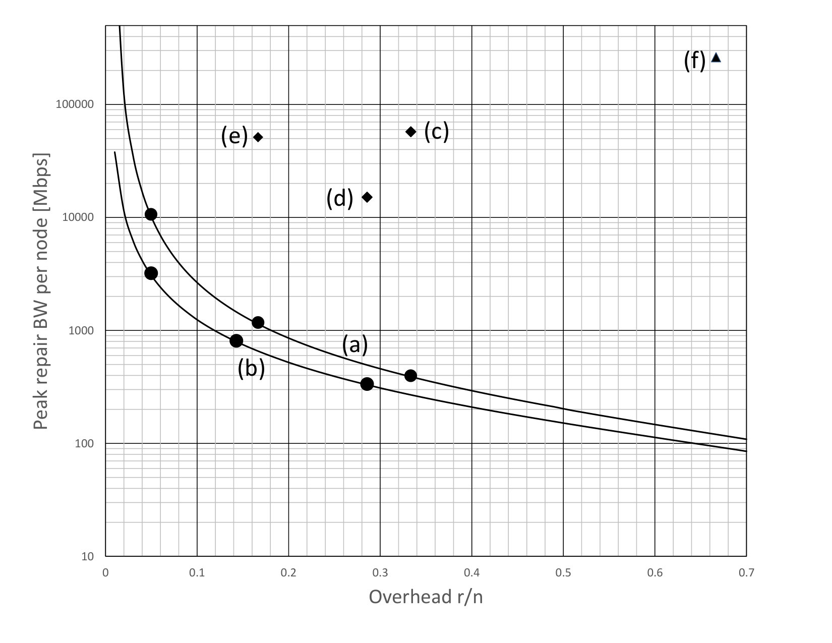 Figure 30
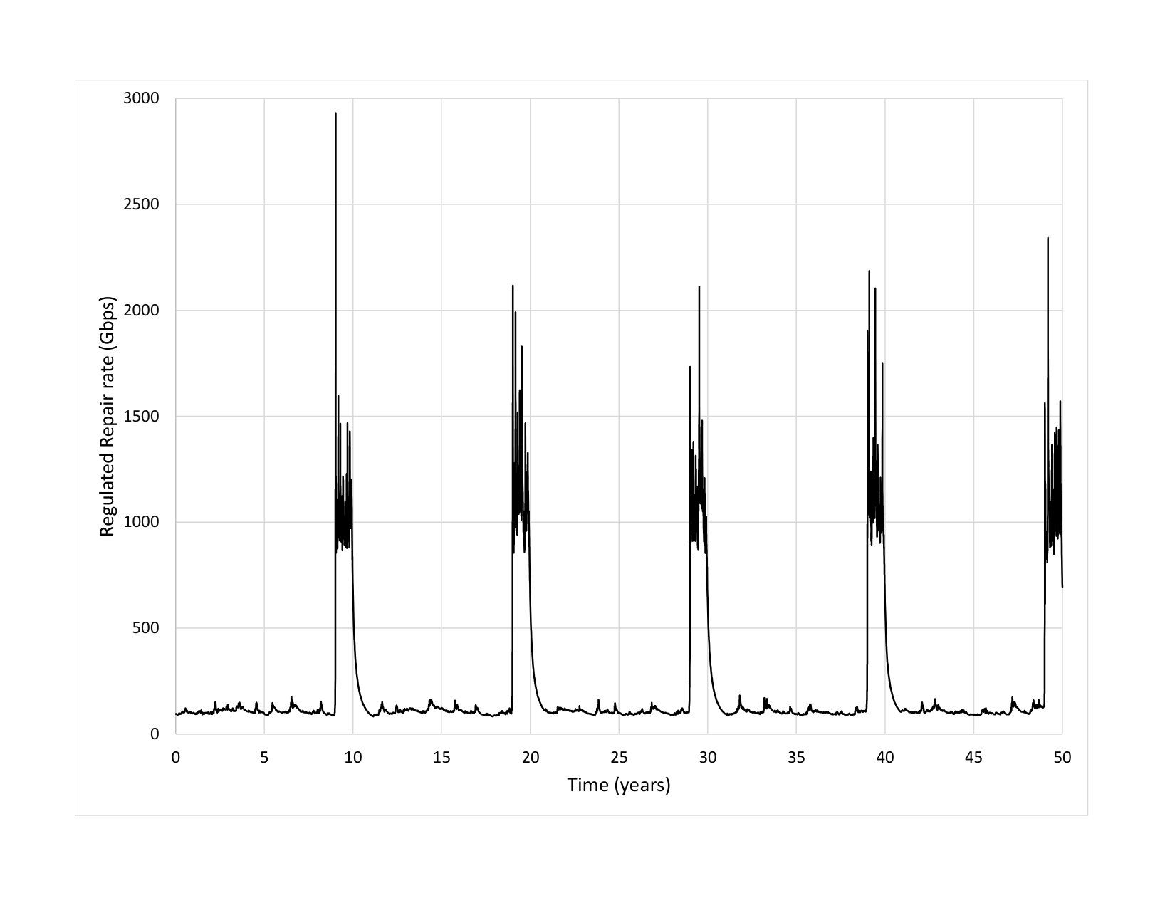 Figure 31
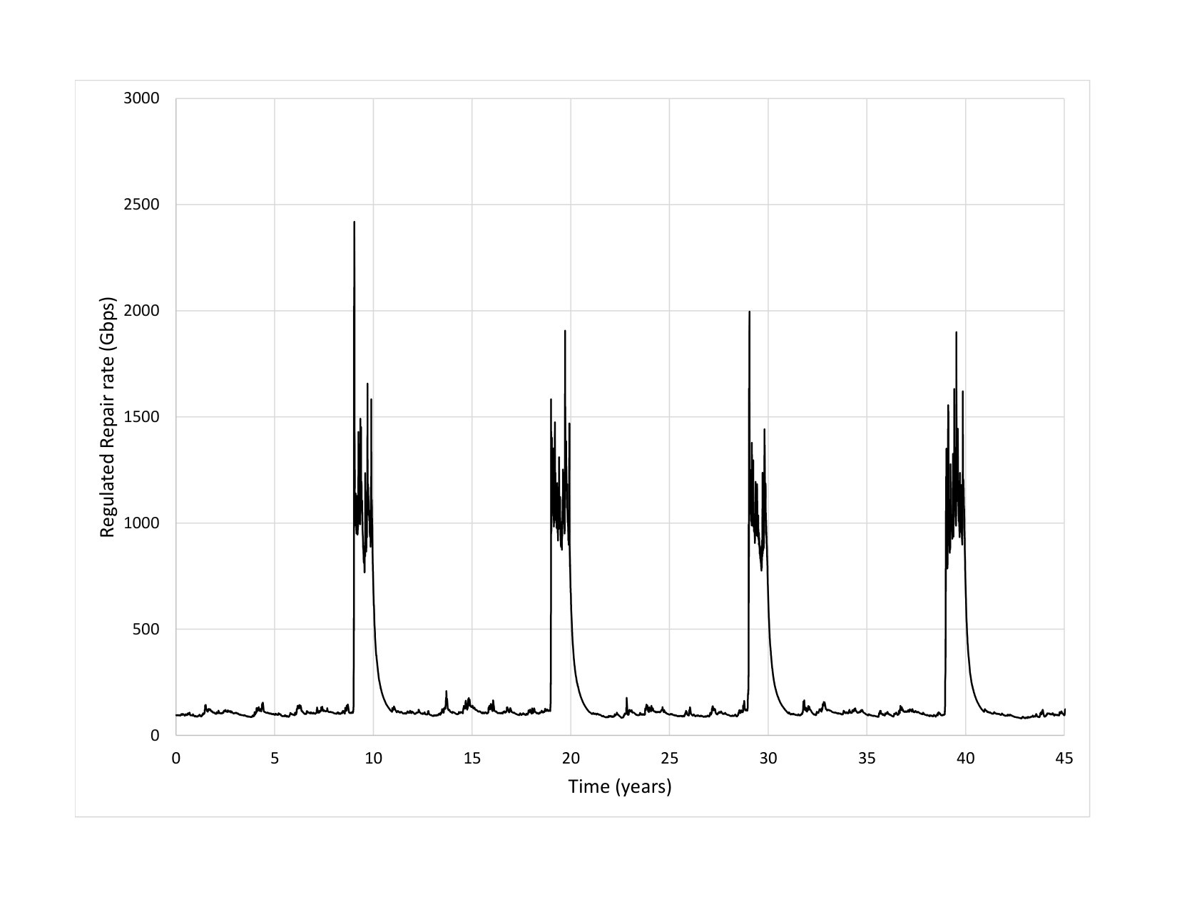 Figure 32
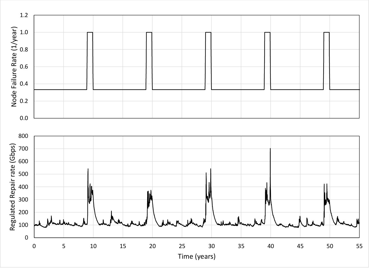 Figure 33
| o — l —— l— l— l —l— l — Number of EFIs used to decode | 1000 | 1001 | 1002 | 1003 | 1004 |
|---|---|---|---|---|---|
| Fraction of failed decodings |
| System parameters | Regulated read repair rate | Fixed read repair rate | ||||||||
|---|---|---|---|---|---|---|---|---|---|---|
| MTTDL | MTTDL | |||||||||
| 402 | 134 | 33.3% | 1 PB | 106 Gbps | 154 Gbps | 226 Gbps | 311 Gbps | years | 104 Gbps | years |
| 402 | 67 | 16.7% | 1 PB | 298 Gbps | 513 Gbps | 975 Gbps | 1183 Gbps | years | 394 Gbps | years |
Peer Reviews
No public reviews on file for this paper yet. If you reviewed it on a platform where reviews are public (OpenReview, ICLR, NeurIPS, ICML), you can paste yours below so the community can read it here.
Videos
No videos yet. Explain this paper in a talk, walkthrough, or lecture? Add one.
Liquid Cloud Storage
Michael G. Luby
Roberto Padovani
Thomas J. Richardson
Lorenz Minder
Pooja Aggarwal
Qualcomm Technologies, Inc. ([email protected])
Qualcomm Technologies, Inc. ([email protected])
Qualcomm Technologies, Inc. ([email protected])
Qualcomm Technologies, Inc. ([email protected])
Qualcomm Technologies, Inc. ([email protected])
Abstract
A liquid system provides durable object storage based on spreading redundantly generated data across a network of hundreds to thousands of potentially unreliable storage nodes. A liquid system uses a combination of a large code, lazy repair, and a flow storage organization. We show that a liquid system can be operated to enable flexible and essentially optimal combinations of storage durability, storage overhead, repair bandwidth usage, and access performance.
keywords:
distributed information systems, data storage systems, data warehouses, information science, information theory, information entropy, error compensation, time-varying channels, error correction codes, Reed-Solomon codes, network coding, signal to noise ratio, throughput, distributed algorithms, algorithm design and analysis, reliability, reliability engineering, reliability theory, fault tolerance, redundancy, robustness, failure analysis, equipment failure.
{CCSXML}
¡ccs2012¿ ¡concept¿ ¡concept_id¿10002951.10003152.10003517.10003519¡/concept_id¿ ¡concept_desc¿Information systems Distributed storage¡/concept_desc¿ ¡concept_significance¿500¡/concept_significance¿ ¡/concept¿ ¡concept¿ ¡concept_id¿10002951.10003152.10003153¡/concept_id¿ ¡concept_desc¿Information systems Information storage technologies¡/concept_desc¿ ¡concept_significance¿100¡/concept_significance¿ ¡/concept¿ ¡concept¿ ¡concept_id¿10002951.10003152.10003166.10003516¡/concept_id¿ ¡concept_desc¿Information systems Storage recovery strategies¡/concept_desc¿ ¡concept_significance¿100¡/concept_significance¿ ¡/concept¿ ¡concept¿ ¡concept_id¿10010520.10010575.10010579¡/concept_id¿ ¡concept_desc¿Computer systems organization Maintainability and maintenance¡/concept_desc¿ ¡concept_significance¿500¡/concept_significance¿ ¡/concept¿ ¡concept¿ ¡concept_id¿10010520.10010575.10010577¡/concept_id¿ ¡concept_desc¿Computer systems organization Reliability¡/concept_desc¿ ¡concept_significance¿300¡/concept_significance¿ ¡/concept¿ ¡concept¿ ¡concept_id¿10010520.10010575.10010578¡/concept_id¿ ¡concept_desc¿Computer systems organization Availability¡/concept_desc¿ ¡concept_significance¿300¡/concept_significance¿ ¡/concept¿ ¡concept¿ ¡concept_id¿10010520.10010575.10010755¡/concept_id¿ ¡concept_desc¿Computer systems organization Redundancy¡/concept_desc¿ ¡concept_significance¿300¡/concept_significance¿ ¡/concept¿ ¡/ccs2012¿
\ccsdesc[500]Information systems Distributed storage \ccsdesc[100]Information systems Information storage technologies \ccsdesc[100]Information systems Storage recovery strategies \ccsdesc[500]Computer systems organization Maintainability and maintenance \ccsdesc[300]Computer systems organization Reliability \ccsdesc[300]Computer systems organization Availability \ccsdesc[300]Computer systems organization Redundancy
\acmformat
1 Introduction
Distributed storage systems generically consists of a large number of interconnected storage nodes, with each node capable of storing a large quantity of data. The key goals of a distributed storage systems are to store as much source data as possible, to assure a high level of durability of the source data, and to minimize the access time to source data by users or applications.
Many distributed storage systems are built using commodity hardware and managed by complex software, both of which are subject to failure. For example, storage nodes can become unresponsive, sometimes due to software issues where the node can recover after a period of time (transient node failures), and sometimes due to hardware failure in which case the node never recovers (node failures). The paper [8] provides a more complete description of different types of failures.
A sine qua non of a distributed storage system is to ensure that source data is durably stored, where durability is often characterized in terms of the mean time to the loss of any source data (MTTDL) often quoted in millions of years. To achieve this in the face of component failures a fraction of the raw storage capacity is used to store redundant data. Source data is partitioned into objects, and, for each object, redundant data is generated and stored on the nodes. An often-used trivial redundancy is triplication in which three copies of each object are stored on three different nodes. Triplication has several advantages for access and ease of repair but its overhead is quite high: two-thirds of the raw storage capacity is used to store redundant data. Recently, Reed-Solomon (RS) codes have been introduced in production systems to both reduce storage overhead and improve MTTDL compared to triplication, see e.g., [10], [8], and [19]. As explained in [19] the reduction in storage overhead and improved MTTDL achieved by RS codes comes at the cost of a repair bottleneck [19] which arises from the significantly increased network traffic needed to repair data lost due to failed nodes.
The repair bottleneck has inspired the design of new types of erasure codes, e.g., local reconstruction codes (LR codes) [9], [19], and regenerating codes (RG codes) [6], [7], that can reduce repair traffic compared to RS codes. The RS codes, LR codes and RG codes used in practice typically use small values of , which we call small codes. Systems based on small codes, which we call small code systems, therefore spread data for each object across a relatively small number of nodes. This situation necessitates using a reactive repair strategy where, in order to achieve a large MTTDL, data lost due to node failures must be quickly recovered. The quick recovery can demand a large amount network bandwidth and the repair bottleneck therefore remains.
These issues and proposed solutions have motivated the search for an understanding of tradeoffs. Tradeoffs between storage overhead and repair traffic to protect individual objects of small code systems are provided in [6], [7]. Tradeoffs between storage overhead and repair traffic that apply to all systems are provided in [14].
Initially motivated to solve the repair bottleneck, we have designed a new class of distributed storage systems that we call liquid systems: Liquid systems use large codes to spread the data stored for each object across a large number of nodes, and use a lazy repair strategy to slowly repair data lost from failed nodes.111The term liquid system is inspired by how the repair policy operates: instead of reacting and separately repairing chunks of data lost from each failed node, the lost chunks of data from many failed nodes are lumped together to form a “liquid” and repaired as a flow. In this paper we present the design and its most important properties. Some highlights of the results and content of paper include:
- •
Liquid systems solve the repair bottleneck, with less storage overhead and larger MTTDL than small code systems.
- •
Liquid systems can be flexibly deployed at different storage overhead and repair traffic operating points.
- •
Liquid systems avoid transient node failure repair, which is unavoidable for small code systems.
- •
Liquid systems obviate the need for sector failure data scrubbing, which is necessary for small code systems.
- •
Liquid system regulated repair provides an extremely large MTTDL even when node failures are essentially adversarial.
- •
Simulation results demonstrate the benefits of liquid systems compared to small code systems.
- •
Liquid system prototypes demonstrate improved access speeds compared to small code systems.
- •
Detailed analyses of practical differences between liquid systems and small code systems are provided.
- •
Liquid systems performance approach the theoretical limits proved in [14].
2 Overview
2.1 Objects
We distinguish two quite different types of data objects. User objects are organized and managed according to semantics that are meaningful to applications that access and store data in the storage system. Storage objects refers to the organization of the source data that is stored, managed and accessed by the storage system. This separation into two types of objects is common in the industry, e.g., see [3]. When user objects (source data) are to be added to the storage system, the user objects are mapped to (often embedded in) storage objects and a record of the mapping between user objects and storage objects is maintained. For example, multiple user objects may be mapped to consecutive portions of a single storage object, in which case each user object constitutes a byte range of the storage object. The management and maintenance of the mapping between user objects and storage objects is outside the scope of this paper.
The primary focus of this work is on storing, managing and accessing storage objects, which hereafter we refer to simply as objects. Objects are immutable, i.e., once the data in an object is determined then the data within the object does not change. Appends to objects and deletions of entire objects can be supported. The preferred size of objects can be determined based on system tradeoffs between the number of objects under management and the granularity at which object repair and other system operations are performed. Generally, objects can have about the same size, or at least a minimum size, e.g., GB. The data size units we use are KB = bytes, MB = KB, GB = MB, TB = GB, and PB = TB.
2.2 Storage and repair
The number of nodes in the system at any point in time is denoted by , and the storage capacity of each node is denoted by , and thus the overall raw capacity is . The storage overhead expressed as a fraction is , and expressed as a per cent is , where is the aggregate size of objects (source data) stored in the system.
When using an erasure code, each object is segmented into source fragments and an encoder generates repair fragments from the source fragments. An Encoding Fragment ID, or EFI, is used to uniquely identify each fragment of an object, where EFIs identify the source fragments of an object, and EFIs identify the repair fragments generated from source fragments. Each of these fragments is stored at a different node. An erasure code is MDS (maximum distance separable) if the object can be recovered from any of the fragments.
A placement group maps a set of fragments with EFIs to a set of of the nodes. Each object is assigned to one of the placement groups, and the selected placement group determines where the fragments for that object are to be stored. To ensure that an equal amount of data is stored on each node, each placement group should be assigned an equal amount of object data and each node should accommodate the same number of placement groups.
For the systems we describe, and thus , i.e., the amount of source data stored in the system is maximized subject to allotting enough space to store fragments for each object. Object loss occurs when the number of fragments available for an object is less than , and thus the object is no longer recoverable. A repairer is an agent that maintains recoverability of objects by reading, regenerating and writing fragments lost due to node failures, to ensure that each object has at least available fragments. In principle the repairer could regenerate missing fragments for an object when only fragments remain available. However, this repair policy results in a small MTTDL, since one additional node failure before regenerating the missing fragments for the object causes object loss.
A repairer determines the rate at which repair occurs, measured in terms of a read repair rate, since data read by a repairer is a fair measure of repair traffic that moves through the network. (The amount of data written by a repairer is essentially the same for all systems, and is generally a small fraction of data read by a repairer.)
Of primary interest is the amount of network bandwidth that needs to be dedicated to repair to achieve a given MTTDL for a particular system, as this value of determines the network infrastructure needed to support repair for the system. Generally, we set a global upper bound on the allowable read repair rate used by a repairer, and determine the MTTDL achieved for this setting of by the system. The average read repair rate is also of some interest, since this determines the average amount of repair traffic moved across the network over time.
The fixed-rate repair policy works in similar ways for small code systems and liquid systems in our simulations: The repairer tries to use a read repair rate up to whenever there are any objects to be repaired.
2.3 Small code systems
Replication, where each fragment is a copy of the original object is an example of a trivial MDS erasure code. For example, triplication is a simple MDS erasure code, wherein the object can be recovered from any one of the three copies. Many distributed storage systems use replication.
A Reed-Solomon code (RS code) [2], [17], [12] is an MDS code that is used in a variety of applications and is a popular choice for storage systems. For example, the small code systems described in [8], [10] use a RS code, and those in [19] use a RS code.
When using a small code for a small code system with nodes, an important consideration is the number of placement groups to use. Since a large number of placement groups are typically used to smoothly spread the fragments for the objects across the nodes, e.g., Ceph [22] recommends . A placement group should avoid mapping fragments to nodes with correlated failures, e.g., to the same rack and more generally to the same failure domain. Pairs of placement groups should avoid mapping fragments to the same pair of nodes. Placement groups are updated as nodes fail and are added. These and other issues make it challenging to design placement groups management for small code systems.
Reactive repair is used for small code systems, i.e., the repairer quickly regenerates fragments as soon as they are lost from a failed node (reading fragments for each object to regenerate the one missing fragment for that object). This is because, once a fragment is lost for an object due to a node failure, the probability of additional node failures over a short interval of time when is small is significant enough that repair needs to be completed as quickly as practical. Thus, the peak read repair rate is higher than the average read repair rate , and is times the node failure erasure rate. In general, reactive repair uses large bursts of repair traffic for short periods of time to repair objects as soon as practical after a node storing data for the objects is declared to have permanently failed.
The peak read repair rate and average read repair rate needed to achieve a large MTTDL for small code systems can be substantial. Modifications of standard erasure codes have been designed for storage systems to reduce these rates, e.g., local reconstruction codes (LR codes) [9], [19], and regenerating codes (RG codes) [6], [7]. Some versions of LR codes have been used in deployments, e.g., by Microsoft Azure [10]. The encoding and decoding complexity of RS, LR, and RG codes grows non-linearly (typically quadratric or worse) as the values of grow, which makes the use of such codes with large values of less practical.
2.4 Liquid systems
We introduce liquid systems for reliably storing objects in a distributed set of storage nodes. Liquid systems use a combination of a large code with large values of , lazy repair, and a flow storage organization. Because of the large code size the placement group concept is not of much importance: For the purposes of this paper we assume that one placement group is used for all objects, i.e., and a fragment is assigned to each node for each object.
The RaptorQ code [20], [13] is an example of an erasure code that is suitable for a liquid system. RaptorQ codes are fundamentally designed to support large values of with very low encoding and decoding complexity and to have exceptional recovery properties. Furthermore, RaptorQ codes are fountain codes, which means that as many encoded symbols as desired can be generated on the fly for a given value of . The fountain code property provides flexibility when RaptorQ codes are used in applications, including liquid systems. The monograph [20] provides a detailed exposition of the design and analysis of RaptorQ codes.
The value of for a liquid system is large, and thus lazy repair can be used, where lost fragments are repaired at a steady background rate using a reduced amount of bandwidth. The basic idea is that the read repair rate is controlled so that objects are typically repaired when a large fraction of fragments are missing (ensuring high repair efficiency), but long before fragments are missing (ensuring a large MTTDL), and thus the read repair rate is not immediately reactive to individual node failures. For a fixed node failure rate the read repair rate can in principle be fixed as described in Appendix A. When the node failure rate is unknown a priori, the algorithms described in Section 9 and Appendix A should be used to adapt the read repair rate to changes in conditions (such as node failure rate changes) to ensure high repair efficiency and a large MTTDL.
We show that a liquid system can be operated to enable flexible and essentially optimal combinations of storage durability, storage overhead, repair bandwidth usage, and access performance, exceeding the performance of small code systems.
Information theoretic limits on tradeoffs between storage overhead and the read repair rate are introduced and proved in [14]. The liquid systems for which prototypes and simulations are described in this paper are similar to the liquid systems described in Section 9.A of [14] that are within a factor of two of optimal. More advanced liquid systems similar to those described in Section 9.B of [14] that are asymptotically optimal would perform even better.
Fig. 1 shows a possible liquid system architecture. In this architecture, a standard interface, such as the S3 or SWIFT API, is used by clients to make requests to store and access objects. Object storage and access requests are distributed across access proxy servers within the liquid access tier. Access proxy servers use a RaptorQ codec to encode objects into fragments and to decode fragments into objects, based on the flow storage organization. Access proxy servers read and write fragments from and to the storage servers that store the fragments on disks within the liquid storage tier. Lazy repair operates as a background process within the liquid storage tier. Further details of this example liquid system architecture are discussed in Section 8.
3 System failures
Since distributed storage systems consist of a large number of components, failures are common and unavoidable. The use of commodity hardware can additionally increase the frequency of failures and outages, as can necessary maintenance and service operations such as software upgrades or system reconfiguration on the hardware or software level.
Different failure types can affect the system in various ways. For example, a hard drive can fail in its entirety, or individual sectors of it can become unreadable. Node failures can be permanent, e.g. if the failure results in the entire node needing to be replaced, or it can be transient, if it is caused issues such as network outages, reboots, software changes. Network failures can cause subsets of many nodes to be unreachable, e.g. a full rack or even a complete site.
Moreover, distributed storage systems are heterogeneous in nature, with components that are commonly being upgraded and replaced. Device models do not remain the same; for example, a replacement hard drive will often be of a different kind, with different and possibly unknown expected lifetime. Even within a device model, different manufacturing runs can result in variation in expected lifetimes. Further, upgrades may require a large set of machines to be replaced in a short time frame, leading to bursts of increased churn. Changes to the underlying technology, such as a transition from hard drives to SSDs, are also likely to profoundly impact the statistics and nature of storage failures.
For these reasons, the failure behavior of a distributed storage system is difficult to model. Results obtained under complicated realistic error models are difficult to interpret, and hard to generalize. The results in this paper are obtained under a fairly straightforward failure model which focuses on two types of failures: Node failures and sector failures.
3.1 Node failures
Although node failure processes can be difficult to accurately model, analysis based on a random node failure models can provide insight into the strengths and weaknesses of a practical system, and can provide a first order approximation to how a practical system will operate. The time till failure of an individual node is often modeled by a Poisson random variable with rate , in which case the average time till an individual node fails is Nodes are assumed to fail independently. Since failed nodes are immediately replaced, the aggregate node failure process is Poisson with rate . Our simulations use this model with years, and also use variants of this model where the node failure rate bursts to times this rate ( year) or times this rate ( years) for periods of time.
Nodes can become unresponsive for a period of time and then become responsive again (transient node failure), in which case the data they store is temporarily unavailable, or nodes can become and remain unresponsive (node failure), in which case the data they store is permanently unavailable. Transient node failures are an order of magnitude more common than node failures in practice, e.g., see [8].
Unresponsive node are generally detected by the system within a few seconds. However, it is usually unknown whether the unresponsiveness is due to a transient node failure or a node failure. Furthermore, for transient node failures, their duration is generally unknown, and can vary in an extremely large range: Some transient node failures have durations of just seconds when others can have durations of months, e.g., see [8].
Section 9 discusses more general and realistic node failure models and introduces repair strategies that automatically adjust to such models.
3.2 Sector failures
Sector failures are another type of data loss that occurs in practice and can cause operational issues. A sector failure occurs when a sector of data stored at a node degrades and is unreadable. Such data loss can only be detected when an attempt is made to read the sector from the node. (The data is typically stored with strong checksums, so that the corruption or data loss becomes evident when an attempt to read the data is made.) Although the sector failure data loss rate is fairly small, the overhead of detecting these types of failures can have a negative impact on the read repair rate and on the MTTDL.
Data scrubbing is often employed in practice to detect sector failures: An attempt is made to read through all data stored in the system at a regular frequency. As an example, [4] reports that Dropbox scrubs data at the frequency of once each two weeks, and reports that read traffic due to scrubbing can be greater than all other read data traffic combined. Most (if not all) providers of data storage systems scrub data, but do not report the frequency of scrubs. Obviously, scrubbing can have an impact on system performance.
The motivation for data scrubbing is that otherwise sector failures could remain undetected for long periods of time, and thus have a large negative impact on the MTTDL. This impact can be substantial even if the data loss rate due to sector failures is relatively much smaller than the data loss rate due to node failures. The reason for this is that time scale for detecting and repairing sector failures is so much higher than for detecting and repairing node failures.
We do not employ a separate scrubbing process in our simulations, but instead rely on the repair process to scrub data: Since each node fails on average in years, data on nodes is effectively scrubbed on average each years. Sector failures do not significantly affect the MTTDL of liquid systems, but can have a significant affect on the MTTDL for small code systems.
We model the time to sector failure of an individual KB sector of data on a node as a Poisson random variable with rate , and thus the average time till an individual KB sector of data on a node experiences a sector failure is , where sector failures of different sectors are independent. Based on sector failure statistics derived from the data of [25], our simulations use this model with years. Thus, the data loss rate due to sector failures is more than times smaller than the data loss rate due to node failures in our simulations.
4 Repair
Although using erasure coding is attractive in terms of reducing storage overheads and improving durability compared to replication, it can potentially require large amounts of bandwidth to repair for fragment loss due to node failures. Since the amount of required repair bandwidth can be high and can cause system-wide bottlenecks, this is sometimes referred to as a repair bottleneck. For example, [19] states the goal of their work as follows:
Our goal is to design more efficient coding schemes that would allow a large fraction of the data to be coded without facing this repair bottleneck. This would save petabytes of storage overheads and significantly reduce cluster costs.
The repair bottleneck sometimes has proven to be an obstacle in the transition from simple replication to more storage efficient and durable erasure coding in storage clusters. It simply refers to the fact that, when using a standard erasure code such as a RS code, the loss of a fragment due to a node failure requires the transfer of fragments for repair, thus increasing -fold the required bandwidth and I/O operations in comparison to replication. For example, [19] states the following when describing a deployed system with 3000 nodes:
…the repair traffic with the current configuration is estimated around 10-20% of the total average of 2 PB/day cluster network traffic. As discussed, (14,10,4) RS encoded blocks require approximately 10x more network repair overhead per bit compared to replicated blocks. We estimate that if 50% of the cluster was RS encoded, the repair network traffic would completely saturate the cluster network links.
The recognition of a repair bottleneck presented by the use of standard MDS codes, such as RS codes, has led to the search for codes that provide locality, namely where the repair requires the transfer of fragments for repair. The papers [9], [10], [19] introduce LR codes and provide tradeoffs between locality and other code parameters. We discuss some properties of small code systems based on LR codes in Section 5.2.
The following sub-sections provide the motivation and details for the repair strategies employed in our simulations.
4.1 Repair initiation timer
In practice, since the vast majority of unresponsive nodes are transient node failures, it is typical to wait for a repair initiation time after a node becomes unresponsive before initiating repair. For example, minutes for the small code system described in [10], and thus the policy reaction is not immediate but nearly immediate.
In our simulations repairers operate as follows. If a node is unresponsive for a period at most then the event is classified as a transient node failure and no repair is triggered. After being unresponsive for a period of time, a node failure is declared, the node is decommissioned, all fragments stored on the node are declared to be missing (and will be eventually regenerated by the repairer). The decommissioned node is immediately replaced by a new node that initially stores no data (to recover the lost raw capacity).
Transient node failures may sometimes take longer than minutes to resolve. Hence, to avoid unnecessary repair of transient node failures, it is desirable to set longer, such as hours. A concern with setting large is that this can increase the risk of source data loss, i.e., it can significantly decrease the
Since a large value for has virtually no impact on the MTTDL for liquid systems, we can set to a large value and essentially eliminate the impact that transient node failures have on the read repair rate. Since a large value for has a large negative impact on the MTTDL for small code systems, must be set to a small value to have a reasonable MTTDL, in which case the read repair rate can be adversely affected if the unresponsive time period for transient node failure extends beyond and triggers unnecessary repair. We provide some simulation results including transient node failures in Section 5.4.
4.2 Repair strategies
In our simulations, a repairer maintains a repair queue of objects to repair. An object is added to the repair queue when at least one of the fragments of the object have been determined to be missing. Whenever there is at least one object in the repair queue the repair policy works to repair objects. When an object is repaired, at least fragments are read to recover the object and then additional fragments are generated from the object and stored at nodes which currently do not have fragments for the object.
Objects are assigned to placement groups to determine which nodes store the fragments for the objects. Objects within a placement group are prioritized by the repair policy: objects with the least number of available fragments within a placement group are the next to be repaired within that placement group. Thus, objects assigned to the same placement group have a nested object structure: The set of available fragments for an object within a placement group is a subset of the set of available fragments for any other object within the placement group repaired more recently. Thus, objects within the same placement group are repaired in a round-robin order. Consecutively repaired objects can be from different placement groups if there are multiple placement groups.
4.3 Repair for small code system
In our simulations, small code systems (using either replication or small codes) use reactive repair, i.e., is set to a significantly higher value than the required average repair bandwidth, and thus repair occurs in a burst when a node failure occurs and the lost fragments from the node are repaired as quickly as possible. Typically only a small fraction of objects are in the repair queue at any point in time for a small code system using reactive repair.
We set the number of placement groups to to the recommended Ceph [22] value, and thus there are placement groups assigned to each of the nodes, with each node storing fragments for placement groups assigned to it. The repair policy works as follows:
- •
If there are at most placement groups that have objects to repair then each such placement group repairs at a read repair rate of .
- •
If there are more than placement groups that have objects to repair then the placement groups with objects with the least number of available fragments are repaired at a read repair rate of .
This policy ensures that, in our simulations, the global peak read repair rate is at most , that the global bandwidth is fully utilized in the typical case when one node fails and needs repair (which triggers placement groups to have objects to repair), and that the maximum traffic from and to each node is not exorbitantly high. (Unlike the case for liquid systems, there are still significant concentrations of repair traffic in the network with this policy.)
The need for small code systems to employ reactive repair, i.e., use a high value, is a consequence of the need to achieve a large MTTDL. Small codes are quite vulnerable, as the loss of a small number of fragments can lead to object loss. For instance, with the RS code the loss of five or more fragments leads to object loss. Fig. 2 illustrates the drastically different time scales at which repair needs to operate for a small code system compared to a liquid system. In this example, nodes fail on average every three years and Fig. 2 shows the probability that of nodes are functioning at time when starting with nodes functioning at time zero. As shown, a failed node needs to be repaired within two days to avoid a probability object loss event for a RS code, whereas a failed node needs to be repaired within months for a large code. Note that the storage overhead is the same in these two systems. A similar observation was made in [21].
Exacerbating this for a small code system is that there are many placement groups and hence many combinations of small number of node failures that can lead to object loss, thus requiring a high value to ensure a target MTTDL. For example, for a small code in a node system, and thus an object from the system is lost if any object from any of the placement groups is not repaired before more than four nodes storing fragments for the object fail. Furthermore, a small code system using many placement groups is difficult to analyze, making it difficult to determine the value of that ensures a target MTTDL.
Although small codes outperform replication in both storage overhead and reliability metrics, they require a high value to achieve a reasonable MTTDL, which leads to the repair bottleneck described earlier. For example, used by small code system can be controlled to be a fraction of the total network bandwidth available in the cluster, e.g., of the total available bandwidth is mentioned in [10] and was estimated in [19] to protect a small fraction of the object data with a small code. However, using these fractions of available bandwidth for repair may or may not achieve a target MTTDL. As we show in Section 5 via simulation, small code systems require a large amount of available bandwidth for bursts of time in order to achieve a reasonable target MTTDL, and in many cases cannot achieve a reasonable MTTDL due to bandwidth limitations, or due to operating with a large value.
4.4 Repair for fixed rate liquid system
The simplest repair policy for a liquid system is to use a fixed read repair rate: the value of the peak read repair rate is set and the read repair rate is whenever there are objects in the repair queue to be processed. A liquid system employs a repairer that can be described as lazy: The value of is set low enough that the repair queue contains almost all objects all the time. Overall, a liquid system using lazy repair uses a substantially lower average repair bandwidth and a dramatically lower peak repair bandwidth than a small code system using reactive repair.
There are two primary reasons that a liquid system can use lazy repair: (1) the usage of a large code, i.e., as shown in Fig. 2, the large code has substantially more time to repair than the small code to achieve the same MTTDL; (2) the nested object structure.
A liquid system can store a fragment of each object at each node, and thus uses a single placement group for all objects. For example, using a large code, an object is lost if the system loses more than nodes storing fragments for the object before the object is repaired. Since there is only one placement group the nested object structure implies that if the object with the fewest number of available of fragments can be recovered then all objects can be recovered. This makes it simpler to determine an value that achieves a target MTTDL for a fixed node failure rate. The basic intuition is that the repair policy should cycle through and repair the objects fast enough to ensure that the number of nodes that fail between repairs of the same object is at most . Note that is the time between repairs of the same object when the aggregate size of all objects is and the peak global read repair bandwidth is set to . Thus, the value of should be set so that the probability that there are more than node failures in time is extremely tiny. Eq. (3) from Appendix A provides methodology for determining a value of that achieves a target MTTDL.
Unlike small code systems, wherein must be relatively small, a liquid systems can use large values, which has the benefit of practically eliminating unnecessary repair due to transient failures.
5 Repair simulation results
The storage capacity of each node is PB in all simulations. The system is fully loaded with source data, i.e., , where is the storage overhead expressed as a fraction.
There are node failures in all simulations and node lifetimes are modeled as independent exponentially distributed random variables with parameter Unless otherwise specified, we set to years. When sector failures are also included, sector lifetimes are also exponentially distributed with fixed to years.
At the beginning of each simulation the system is in a perfect state of repair, i.e., all fragments are available for all objects. For each simulation, the peak global read repair bandwidth is limited to a specified value. The MTTDL is calculated as the number of years simulated divided by one more than the observed number of times there was an object loss event during the simulation. The simulation is reinitialized to a perfect repair state and the simulation is continued when there is an object loss event. To achieve accurate estimates of the MTTDL, each simulation runs for a maximum number of years, or until object loss events have occurred.
Fig. 3 presents a comparison of repair traffic for a liquid system and a small code system. In this simulation, lazy repair for the liquid system uses a steady read repair rate of Gbps to achieve an MTTDL of years, whereas the reactive repair for the small code system uses read repair rate bursts of Tbps to achieve an MTTDL slightly smaller than years. For the small code system, a read repair rate burst starts each time a node fails and lasts for approximately hours. One of the nodes fails on average approximately every hours.
In Fig. 4, we plot against achieved MTTDL for a cluster of nodes. The liquid systems use fixed read repair rate equal to the indicated and two cases of and are shown. The curves depict MTTDL bounds as calculated according to Eq. (3) of Appendix A. As can be seen, the bounds and the simulation results agree quite closely. Fig. 4 also shows simulation results for a small code system with storage overhead which illustrates a striking difference in performance between small code systems and liquid systems.
5.1 Fixed node failure rate with nodes
Fig. 5 plots the simulation results for against MTTDL for a wide variety of node systems. Each simulation was run for years or until object loss events occurred. The number of nodes, the node failure rate, and the small codes used in these simulations are similar to [10]. The square icons correspond to storage overhead and the circle icons correspond to storage overhead. For the small code systems, a small code is used for storage overhead, and a small code is used for storage overhead. For the liquid systems, a large code is used for storage overhead, and a large code is used for storage overhead.
The unshaded icons correspond to systems where there are only node failures, whereas the shaded icons correspond to systems where there are both node failures and sector failures.
The small code systems labeled as “SC, 30min” and “SC, 24hr” use the read repair rate strategy described in Section 4.3 based on the indicated value, with set to 30 minutes and 24 hours respectively. The triplication systems labeled as “Trip, 30min” and “Trip, 24hr” use the read repair rate strategy described in Section 4.3 based on the indicated value with is set to 30 minutes and 24 hours respectively.
The liquid systems labeled as “LiqF, 24hr” use a fixed read repair rate set to the shown , which was calculated according to Eq. (3) from Appendix A with a target MTTDL of years. The value of is set to 24 hours As would be expected since Eq. (3) is a lower bound, the observed MTTDL in the simulations is somewhat above years.
The liquid systems labeled as “LiqR, 24hr” have set to 24 hours and use a version of the regulator algorithm described in Section 9 to continually and dynamically recalculate the read repair rate according to current conditions. The regulator used (per object) node failure arrival rate estimates based on the average of the last node failure inter-arrival times where denotes the number of missing fragments for an object at the time it forms the estimate. The maximum read repair rate was limited to the shown value, which is about three times the average rate. In these runs there were no object loss events in the years of simulation when there are both node failures and sector failures. This is not unexpected, since the estimate (using the MTTDL lower bound techniques described in Section 9 but with a slightly different form of node failure rate estimation) for the actual MTTDL is above years for the storage overhead case and above years for the storage overhead case. These estimates are also known to be conservative when compared to simulation data. The same estimate shows that with this regulator an MTTDL of years would be attained with the smaller overhead of instead of . As shown in Table 2, the average read repair rate is around of , and the read repair rate is around of . The large MTTDL achieved by the regulator arises from its ability to raise the repair rate when needed. Other versions of the regulator in which the peak read repair rate is not so limited can achieve much larger MTTDL. For example, a version with a read repair rate limit set to be about five times the average rate for the given node failure rate estimate achieves an MTTDL of around years for the storage overhead case.
As can be seen, the value of required for liquid systems is significantly smaller than that required for small code systems and for triplication. Furthermore, although regulated rate liquid system can provide an MTTDL of greater than years even when is set to hours and there are sector failures in addition to node failures, the small code systems and triplication do not provide as good an MTTDL even when is set to minutes and there are no sector failures, and provide a poor MTTDL when is set to hours or when there are sector failures. The MTTDL would be further degraded for small code systems if both were set to 24 hours and there were sector failures.
5.2 Fixed node failure rate with nodes
Fig. 6 shows detailed simulation results, plotting the value of and the resulting value of MTTDL for various node systems. Each simulation was run for years or until object loss events occurred. The number of nodes, the node failure rate, and the small code systems used in these simulations are similar to [19]. The square icons correspond to storage overhead and the circle icons correspond to storage overhead. For the small code systems, a small code is used for storage overhead, and a small code is used for storage overhead. For the liquid systems, a large code is used for storage overhead, and a large code is used for storage overhead. The remaining parameters and terminology used in Fig. 6 are the same as in Fig. 5. There were no object loss events in the years of simulation for any of the liquid systems shown in Fig. 6.
The systems “LiqR, 24hr” liquid systems used a regulated repair rate similar to that described for the 402 node system described above. The target repair efficiency was set at In this case the average repair rate is higher than for the fixed rate case because the fixed rate case was set using the target MTTDL which, due the larger scale, admits more efficient repair than the 402 node system for the same target MTTDL. Estimates of MTTDL for the regulated case using techniques from Section 9 indicate that the MTTDL is greater than an amazing years for the storage overhead case and years for the storage overhead case even without the benefit of node failure rate estimation. As before, the regulated repair system could be run at substantially lower overhead while still maintaining a large MTTDL. For the “LiqR, 24hr” liquid systems, the average read repair rate is around of , and the read repair rate is around of .
The conclusions drawn from comparing small code systems to liquid systems shown in Fig. 5 are also valid for Fig. 6 but to an even greater degree. The benefits of the liquid system approach increase as the system size increases.
The paper [19] describes a repair bottleneck for a small code system, hereafter referred to as the Facebook system, which has around nodes and storage capacity per node of approximately TB. The Facebook system uses a RS code to protect 8% of the source data and triplication to protect the remaining 92% of the source data. The amount of repair traffic estimated in [19] for the Facebook system is around 10% to 20% of the total average of PB/day of cluster network traffic. The paper [19] projects that the network would be completely saturated with repair traffic if even of the source data in the Facebook system were protected by the RS code.
Taking into account the mix of replicated and RS protected source data and the mixed repair traffic cost for replicated and RS protected source data, there are around to node failures per day in the Facebook system. An average of to node failures per day for a node system implies that each individual node on average fails in around to days, which is around to times the node failure rate of years we use in most of our simulations. If all source data were protected by a RS code in the Facebook system then the repair traffic per day would average around to PB. However, the node failure per day statistics in [19] have wide variations, which supports the conclusions in [19] that protecting most of the source data with the RS code in the Facebook system will saturate network capacity.
Note that to PB/day of repair traffic for the Facebook system implies an average read repair rate of around to Gbps. If the storage capacity per node were PB instead of TB then the Facebook system average read repair rate would be approximately to Tbps, which is around to times the average read repair rate for the very similar “SC, 30min” small code system shown in Fig. 6. This relative difference in the value of makes sense, since the Facebook system node failure rate is around to times larger than for the“SC, 30min” small code system.
The “SC, 30min” small code system shown in Fig. 6 achieves an MTTDL of just under years using a peak read repair rate Tbps and using minutes. Assume the node failure rate for the Facebook system is times the node failure rate for the “SC, 30min” small code system shown in Fig. 6, and suppose we set minutes for the Facebook system. The scaling observations in Section 5.5 show that this Facebook system achieves a MTTDL of just under years when Tbps.
The average node failure rates reported in [19] for the Facebook system are considerably higher than the node failure rates we use in our simulations. One possible reason is that the Facebook system uses a small value, e.g., minutes, after which unresponsive nodes trigger repair. This can cause unnecessary repair of fragments on unresponsive nodes that would have recovered if were larger.
It is desirable to set as large as possible to avoid unnecessary repair traffic, but only if a reasonable MTTDL can be achieved. The results in Fig. 6 indicate that a small code system cannot offer a reasonable MTTDL with hours. On the other hand, the results from Section 5.4 indicate that the average read repair rate increases significantly (indicating a significant amount of unnecessary repair) if a smaller value of is used for a small code system when there are transient node failures. In contrast, a regulated liquid system can provide a very large MTTDL operating with hours and with sector failures, thus avoiding misclassification of transient node failures and unnecessary repair traffic.
Results for small code systems using LR codes [9], [10], [19] can be deduced from results for small code systems using RS codes. A typical LR code (similar to the one described in [10] which defines a LR code) partitions source fragments into two groups of five, generates one local repair fragment per group and two global repair fragments for a total of fragments, and thus the storage overhead is the same as for a RS code. At least five fragments are read to repair a lost fragment using the LR code, whereas fragments are read to repair a lost fragment using the RS code. However, there are fragment loss patterns the LR code does not protect against that the RS code does. Thus, the LR code operating at half the value used for the RS code achieves a MTTDL that is lower than the MTTDL for the RS code.
Similarly, results for [19] which use a LR code can be compared against the RS code that we simulate. The LR code operating at half the value used for the RS code achieves an MTTDL that may be as large as the MTTDL for the RS code. However, the LR code storage overhead is , which is higher than the RS code storage overhead of .
5.3 Varying node failure rate
In this subsection we demonstrate the ability of the regulated repair system to respond to bursty node failure processes. The node failures in all simulations described in this subsection are generated by a time varying periodic Poisson process repeating the following pattern over each ten year period of time: the node failure rate is set to years for the first nine years of each ten year period, and then year for the last year of each ten year period. Thus, in each ten year period, the node failure rate is the same as it was in the previous subsections for the first nine years, followed by a node failure rate that is three times higher for the last year.
Except for using variable for node failures, Fig. 7 is similar to Fig. 5. The small code systems labeled as “SC, 30min” in Fig. 7 use the read repair rate strategy described in Section 4.3 based on the shown value, and is set to 30 minutes. Thus, even when the node failure rate is lower during the first nine years of each period, the small code system still sets read repair rate to whenever repair is needed.
The liquid systems labeled as “LiqR, 24hr” in Fig. 7 use the regulator algorithm described in Section 9 to continually and dynamically recalculate the read repair rate according to current conditions, allowing a maximum read repair rate up to the shown value, and is set to 24 hours. In these runs there were no object loss events in the years of simulation with both node failures and sector failures. [[We may want to compute something here TBD?]]
Fig. 18 is an example trace of the read repair rate as function of time for the liquid system labeled “LiqR, 24hr” in Fig. 7, which shows how the the read repair rate automatically adjusts as the node failure rate varies over time. In these simulations, the average read repair rate is around of during the first nine years of each period and around of during the last year of each period, and the read repair rate is around of during the first nine years of each period and around of during the last year of each period. Thus, the regulator algorithm does a good job of matching the read repair rate to what is needed according to the current node failure rate.
Except for using variable for node failures, Fig. 8 is similar to Fig. 6. The conclusions comparing small code systems to liquid systems shown in Fig. 7 are also valid for Fig. 8.
5.4 Transient node failures
In this subsection we demonstrate the ability of the liquid systems to efficiently handle transient node failure processes.
Fig. 10 plots the simulation results for against MTTDL for a number of node systems. Like in previous subsections, the node lifetimes for node failures are modeled as independent exponentially distributed random variables with parameter and is set to years. The occurrence times of transient node failures are modeled as independent exponentially distributed random variables with parameter and is set to years. Thus, transient node failures occur at times the rate at which node failures occur, consistent with [8]. The durations of transient node failures are modeled with log-logistic random variables, having a median of seconds and shape parameter . These choices were made so as to mimic the distribution provided in [8]. Figure 9 shows the graph from [8] with the log-logistic fitted curve overlaid. With this model, less than of the transient node failures last for more than minutes.
The unshaded markers mark simulations with just node failures and the shaded markers mark simulations with both node failures and transient node failures.
The values in all simulations is the same as value used correspondingly in Fig. 5. The small code systems labeled as “SC, 30min” and “SC, 24hr“ in Fig. 10 use the read repair rate strategy described in Section 4.3, with value of Gbps and is set to 30 minutes and 24 hours respectively. The liquid system labeled as “LiqR, 24hr” in Fig. 10 uses the regulator algorithm described in Section 9, with value of Gbps and is set to 24 hours.
As evident, there is no difference in the for the liquid system between simulations with transient node failures and those without. No object loss events were observed for the liquid system in the years of simulation with both node failures and transient node failures. The for small code system labeled as “SC, 30min“ is however higher for the simulation with transient node failures and achieves an MTTDL that is less than half of what is achieved when there are no transient node failures. The for small code system labeled as “SC, 24hr“ is the same between simulations with transient node failures and those without, but they fail to achieve a high enough MTTDL and do not provide adequate protection against object loss.
Thus, the liquid systems do a better job of handling transient node failures without requiring more effective average bandwidth than small code systems.
5.5 Scaling parameters
The simulation results shown in Section 5 are based on sets of parameters from published literature, and from current trends in deployment practices. As an example of a trend, a few years ago the storage capacity of a node was around TB, whereas the storage capacity of a node in some systems is PB or more, and thus the storage capacity per node has grown substantially.
Repair bandwidths scale linearly as a function of the storage capacity per node (keeping other input parameters the same). For example, the values of for a system with TB can be obtained by scaling down by a factor of two the values of from simulation results for PB, whereas the MTTDL and other values remain unchanged.
Repair bandwidths and the MTTDL scale linearly as a function of concurrently scaling the node failure rate and the repair initiation timer . For example, the values of for a system with years and hours can be obtained by scaling down by a factor of three the values of from simulation results for years and hours, whereas the MTTDL can be obtained by scaling up by a factor of three, and other values remain unchanged.
6 Encoding and decoding objects
In a block storage organization commonly used by small code systems, objects are partitioned into successive source fragments and encoded to generate repair fragments (we assume the small code is MDS). In effect a fragment is a symbol of the small code, although the small code may be intrinsically defined over smaller symbols, e.g., bytes. A high level representation of a block storage organization for a simple example using a Reed-Solomon code is shown in Fig. 11, where the object runs from left to right across the source fragments as indicated by the blue line.
A relatively small chunk of contiguous data from the object that resides within a single source fragment can be accessed directly from the associated node if it is available. If, however, that node is unavailable, perhaps due to a transient node failure or node failure, then corresponding chunks of equal size must be read from other nodes in the placement group and decoded to generate the desired chunk. This involves reading times the size of the missing chunk and performing a decoding operation, which is referred to as a degraded read [19], [18]. Reading chunks can incur further delays if any of the nodes storing the chunks are busy and thus non-responsive. This latter situation can be ameliorated if a number of chunks slightly larger than are requested and decoding initiated as soon as the first chunks have arrived, as described in [11].
A flow storage organization, used by liquid systems, operates in a stream fashion. An large code is used with small symbols of size Ssize, resulting in a small source block of size . For example, with and symbols of size Bytes, a source block is of size KB. An object of size Osize is segmented into
[TABLE]
source blocks, and the source symbols of each such source block is independently erasure encoded into symbols. For each , the fragment with EFI consists of the concatenation of the symbol from each of the consecutive source blocks of the object. An example of a flow storage organization showing a large code with is shown in Fig. 12, where each row corresponds to a source block and runs from left to right across the source symbols as indicated by the dashed blue lines, and the object is the concatenation of the rows from top to bottom.
A chunk of data consisting of a consecutive set of source blocks can be accessed as follows. For a fragment with EFI , the consecutive portion of the fragment that corresponds to the symbol from each of consecutive set of source blocks is read. When such portions from at least fragments are received (each portion size a -fraction of the chunk size), the chunk of data can be recovered by decoding the consecutive set of source blocks in sequence. Thus, the amount of data that is read to access a chunk of data is equal to the size of the chunk of data. Portions from slightly more than fragments can be read to reduce the latency due to nodes that are busy and thus non-responsive. Note that each access requires a decoding operation.
Let us contrast the two organizations with a specific example using an object of size GB. Consider an access request for the MB chunk of the object in positions MB through MB, which is shown as the shaded region in Fig. 13 with respect to both a block storage organization and a flow storage organization.
With the block storage organization shown in Fig. 11, the MB chunk is within the fragment with EFI = as shown in Fig. 13. If the node that stores this fragment is available then the chunk can be read directly from that node. If that node is unavailable, however, then in order to recover the MB chunk the corresponding MB chunks must be retrieved from any six available nodes of the placement group and decoded. In this case a total of MB of data is read and transferred through the network to recover the MB chunk of data.
With the flow storage organization shown in Fig. 12, the chunk of size MB corresponds to consecutive source blocks from source block 9216 to block 9727 as shown in Fig. 13, which can be retrieved by reading the corresponding portion of the fragment from each of at least fragments. From the received portions, the chunk can be recovered by decoding the source blocks. Thus, in a flow storage organization a total of MB of data is read and transferred through the network to recover the original MB chunk of data.
Naturally, the symbol size, source block size, and the granularity of the data to be accessed should be chosen to optimize the overall design, taking into account constraints such as whether the physical storage is hard disk or solid state.
7 Prototype Implementation
Our team implemented a prototype of the liquid system. We used the prototype to understand and improve the operational characteristics of a liquid system implementation in a real world setting, and some of these learnings are described in Section 8. We used the prototype to compare access performance of liquid systems and small code systems. We used the prototype to cross-verify the lazy repair simulator that uses a fixed read repair rate as described in Section 4.4 to ensure that they both produce the same MTTDL under the same conditions. We used the prototype to validate the basic behavior of a regulated read repair rate as described in Section 9.
The hardware we used for our prototype consists of a rack of 14 servers. The servers are connected via 10 Gbit full duplex ethernet links to a switch, and are equipped with Intel Xeon CPUs running at 2.8 GHz, with each CPU having 20 cores. Each server is equipped with an SSD drive of 600 GB capacity that is used for storage.
The liquid prototype system software is custom written in the Go programming language. It consists of four main modules:
- •
Storage Node (SN) software. The storage node software is a HTTP server. It is used to store fragments on the SSD drive. Since a liquid system would generally use many more than 14 storage nodes, we ran many instances of the storage node software on a small number of physical servers, thereby emulating systems with hundreds of nodes.
- •
An Access Generator creates random user requests for user data and dispatches them to accessors. It also collects the resulting access times from the accessors.
- •
Accessors take user data requests from the access generator and create corresponding requests for (full or partial) fragments from the storage nodes. They collect the fragment responses and measure the amount of time it takes until enough fragments have been received to recreate the user data. There are in general multiple accessors running in the system.
- •
A Repair Process is used to manage the repair queue and regenerate missing fragments of stored objects. The repair process can be configured to use a fixed read repair rate, or to use a regulated read repair rate as described in Section 9.
In addition, the team developed a number of utilities to test and exercise the system, e.g., utilities to cause node failures, and tools to collect data about the test runs.
7.1 Access performance setup
The users of the system are modeled by the access generator module. We set a target user access load () on the system as follows. Let be the aggregate capacity of the network links to the storage nodes, and let be the size of the user data requests that will be issued. Then requests per unit of time would use all available capacity. We set the mean time between successive user requests to , so that on average a fraction of the capacity is used. The access generator module uses an exponential random variable to generate the timing of each successive user data request, where the mean of the random variable is .
As an example, there is a 10 Gbps link to each of the six storage nodes in the setup of Fig. 14, and thus Gbps. If user data requests are of size MB bits, and the target load is ( of capacity), then the mean time between requests is set to
[TABLE]
The access generator module round-robins the generated user data requests across the accessor modules. When an accessor module receives a generated user data request from the access generator module, the accessor module is responsible for making fragment requests to the storage nodes and collecting response payloads; it thus needs to be fairly high performance. Our implementation of an accessor module uses a custom HTTP stack, which pipelines requests and keeps connections statically alive over extended periods of time. Fragment requests are timed to avoid swamping the switch with response data and this reduces the risk of packet loss significantly. The server network was also tuned, e.g., the TCP retransmission timer was adjusted for the use case of a local network. See [5] for a more detailed discussion of network issues in a cluster environment. These changes in aggregate resulted in a configuration that has low response latency and is able to saturate the network links fully.
7.2 Access performance tests
The prototype was used to compare access performance of liquid systems and small code systems. Our goal was to evaluate access performance using liquid system implementations, i.e., understand the performance impact of requesting small fragments (or portions of fragments) from a large number of storage servers. For simplicity we evaluated the network impact on access performance. Fragment data was generally in cache and thus disk access times were not part of the evaluation. We also did not evaluate the computational cost of decoding. Some of these excluded aspects are addressed separately in Section 8.
Figure 14 displays the setup that we use for testing access speed. Each physical server has a full duplex 10 GbE network link which is connected over a switch to all the other server blades. Testing shows that we are able to saturate all of the 10 Gbps links of the switch simultaneously. Eight of our 14 physical servers are running accessors, and one of the eight is running the access generator as well. The remaining six servers are running instances of the storage node software. This configuration allows us to test the system under a load that saturates the network capacity to the storage nodes: The aggregate network capacity between the switch and the accessors is 80 Gbps, which is more than the aggregate network capacity of 60 Gbps between the switch and the storage nodes, so the bottleneck is the 60 Gbps between the switch and the storage nodes.
During access performance tests there are no node failures, all fragments for each object are available, and the repair process is disabled. For all tests, storage node instances run on each storage server, which emulates a system of nodes. We operate with a storage overhead of , a large code is used for the liquid system, and a small code is used for the small code system. We tested with MB and MB user data request sizes.
We run the access prototype in three different configurations. The “Liq” configuration models liquid system access of user data. For a user data request of size , the accessor requests fragment portions, each of size , from a random subset of distinct storage nodes, and measures the time until the first complete responses are received (any remaining up to responses are discarded silently by the accessor). Each fragment portion is of size around KB when MB, and around KB when MB. We use , and thus the total size of requested fragment portions is around MB when MB, and around MB when MB. See [11] for an example of this access strategy.
The “SC” configuration models small code system normal access of user data, i.e., the requested user data is stored on a storage node that is currently available. For a user data request of size , the accessor requests one fragment portion of size from a randomly selected storage node, and measures the time until the complete response is received. The total size of the requested fragment portion is MB when MB, and MB when MB.
The “SC-Deg” configuration models small code system degraded access of user data, i.e., the requested user data is stored at a storage node that that is currently unavailable, e.g., see [19], [18]. For a user data request of size , the accessor requests fragment portions of size from a random subset of distinct storage nodes and measures the time until the first complete responses are received. The total size of requested fragment portions is MB when MB, and MB when MB. Most user data is stored at available storage nodes, and thus most accesses are normal, not degraded, in operation of a small code system. Thus, we generate the desired load on the system with normal accesses to user data, and run degraded accesses at a rate that adds only a nominal aggregate load to the system, and only the times for the degraded accesses are measured by the accessors. Similar to the “Liq” configuration, we could have requested fragment portions for the “SC-Deg” configuration to decrease the variation in access times, but at the expense of even more data transfer over the network.
Figures 15 and 16 depict access time results obtained with the above settings under different system loads. The average time for liquid system accesses is less than for small code system normal accesses in most cases, except under very light load when they are similar on average. Even more striking, the variation in time is substantially smaller for liquid systems than for small code systems under all loads. Liquid system accesses are far faster (and consume less network resources) than small code system degraded accesses.
Our interpretation of these results is that liquid systems spread load equally, whereas small code systems tend to stress individual storage nodes unevenly, leading to hotspots. With small code systems, requests to heavily loaded nodes result in slower response times. Hotspots occur in small code systems when appreciably loaded, even when the fragment requests are distributed uniformly at random. It should be expected that if the requests are not uniform, but some data is significantly more popular than other data, then response times for small code systems would be even more variable.
7.3 Repair tests and verification of the simulator
We used the prototype repair process to verify our liquid system repair simulator. We started from realistic sets of parameters, and then sped them up by a large factor (e.g., 1 million), in such a way that we could run the prototype repair process and observe object loss in a realistic amount of time. We ran the prototype repair process in such a configuration, where node failures were generated artificially by software. The resulting measured statistics, in particular the MTTDL, were compared to an equivalent run of the liquid system repair simulator. This allowed us to verify that the liquid system repair simulator statistics matched those of the prototype repair process and also matched our analytical predictions.
8 Implementation considerations
Designing a practical liquid system poses some challenges that are different from those for small code systems. In the following sections we describe some of the issues, and how they can be addressed.
8.1 Example Architecture
As discussed in Section 2.4, Fig. 1 shows an example of a liquid system architecture. This simplified figure omits components not directly related to source data storage, such as system management components or access control units.
Concurrent capacity to access and store objects scales with the number of access proxy servers, while source data storage capacity can be increased by adding more storage nodes to the system, and thus these capacities scale independently with this architecture. Storage nodes (storage servers) can be extremely simple, as their only function is to store and provide access to fragments, which allows them to be simple and inexpensive. The lazy repair process is independent of other components; thus reliability is handled by a dedicated system.
8.2 Metadata
The symbol size used by a liquid system with a flow storage organization is substantially smaller than the size used by a small code system with a block storage organization. For a small code system each symbol is a fragment, whereas for a liquid system there are many symbols per fragment and, as described in Section 6, the symbol to fragment mapping can be tracked implicitly. For both types of systems, each fragment can be stored at a storage node as a file.
The names and locations of each fragment are explicitly tracked for small code systems. There are many more fragments to track for a liquid system because of the use of a large code, and explicit tracking is less appealing. Instead, a mapping from the placement group to available nodes can be tracked, and this together with a unique name for each object can be used to implicitly derive the names and locations of fragments for all objects stored at the nodes for liquid systems.
8.3 Network usage
The network usage of a liquid system is fairly different from that of a small code system. As described in Section 7.2, liquid systems use network resources more smoothly than small code systems, but liquid systems must efficiently handle many more requests for smaller data sizes. For example, a small code system using TCP might open a new TCP connection to the storage node for each user data request. For a liquid system, user data requests are split into many smaller fragment requests, and opening a new TCP connection for each fragment request is inefficient. Instead, each access proxy can maintain permanent TCP connections to each of the storage nodes, something that modern operating systems can do easily. It is also important to use protocols that allow pipeline data transfers over the connections, so that network optimizations such as jumbo packets can be effectively used. For example the HTTP/2 protocol [1] satisfies these properties.
Technologies such as RDMA [16] can be used to eliminate processing overhead for small packets of data. For example, received portions of fragments can be placed autonomously via RDMA in the memory of the access proxy, and the access proxy can decode or encode one or more source blocks of data concurrently.
8.4 Storage medium
A key strength of liquid systems is that user data can be accessed as a stream, i.e., there is very little startup delay until the first part of a user data request is available, and the entire user data request is available with minimal delay, e.g., see Section 7.2. Nevertheless, random requests for very small amounts of user data is more challenging for a liquid system.
The storage medium used at the storage nodes is an important consideration when deciding the large code parameters . Hard disk drives (HDDs) efficiently support random reads of data blocks of size 500 KB or larger, whereas solid state drives (SSDs) efficiently support random reads of data blocks of size 4 KB or larger. We refer to these data block sizes as the basic read size of the storage medium. The parameters should be chosen so that if is the typical requested user data size then is at least the basic read size, which ensures that a requested fragment portion size is at least the basic read size. In many cases this condition is satisfied, e.g., when the requested user data size is generally large, or when the storage medium is SSD.
In other cases, more advanced methods are required to ensure that a liquid system is efficient. For example, user data request performance can be improved by assigning different size user data to different types of objects: Smaller user data is assigned to objects that are stored using smaller values of , and larger user data is assigned to objects that are stored using larger values of , where in each case is at least the basic read size if is the requested user data size. In order to achieve a large MTTDL for all objects, the storage overhead is set larger for objects stored using smaller values of than for objects stored using larger values of . Overall, since the bulk of the source data is likely to be large user data, the overall storage overhead remains reasonable with this approach.
Only a small proportion of user data is frequently accessed in many use cases, e.g., in the use case described in [15], only about 10% of the user data is accessed frequently, and this user data is easy to identify based on the amount of time it has been stored in the storage system. Thus, a caching layer can be used to store and make such user data available without having to request the user data from the storage system. For a liquid system, it makes most sense to cache user data that is both small and frequently accessed.
Another strategy to minimize requests for small user data is to store related user data together in objects and coalesce accesses. Suppose for example, the storage system stores web content. To load a web page, dozens of small files of user data are typically loaded, such as HTML content and small images. Since the same content is accessed whenever such a web page is displayed, the system can store and access this user data together.
8.5 RaptorQ software performance
With small code systems, user data can usually be accessed directly without requiring erasure decoding. With liquid systems, each access of user data typically requires erasure decoding.
RaptorQ codes are the large codes of choice for liquid systems. The encoding and decoding complexity of RaptorQ codes is inherently linear by design [20], i.e., for a RaptorQ code, the encoding complexity is linear in , and the decoding complexity is linear in , which makes the use of a RaptorQ code with large values of practical.
Software implementations of RaptorQ codes have been deployed in a number of applications, including real-time applications that require low encoding and decoding complexity. Encode and decode speeds of over 10 Gbps are achieved using a software implementation of RaptorQ running on one core of a 20 core Intel Xeon CPU ES-2680 server running at 2.8 GHz, with code parameters and 256 byte symbols. Aggregate encode and decode speeds of around 150 Gbps are achieved using all 20 cores of the same server, with the same code parameters and symbol size.
These numbers suggest that RaptorQ decoding would add a fractional extra cost to the data processing pipeline: It is expected that other transformations are performed when accessing user data, such as for example checksumming, decompression and decryption. Of those MD5 checksums can be computed on the same machine at a rate of at most about 4 Gbps. As for decompression, Google’s run-time performance oriented Snappy codec achieves reportedly about 4 Gbps on a Core i7 processor [23], suggesting that RaptorQ coding is not a bottleneck.
8.6 RaptorQ hardware performance
Hardware based implementations have the potential to further cut down on power usage by the RaptorQ codes. Based on a hardware RaptorQ code chip design by Qualcomm for a different application, our estimate is that the power usage in an ASIC implementation would be about 3 Watts per 100 Gbps encoding or decoding speed.
To put this into perspective, we compare this to the power use of an SSD to access data. For example, the Samsung SM863a 2 TB enterprise SSD drive [24], achieves a data transfer rate of up to about 4.1 Gbps and uses about 2.5 W of power when reading. This translates to a power use of about 61 W to achieve 100 Gbps. Thus, the power needed for the RaptorQ code is about 5% of the power needed to read the data off a drive. If other necessary aspects such as network transfer, etc, were incorporated as well, the RaptorQ code share drops well below 5%.
8.7 RaptorQ decode reliability
Extremely high durability is required for storage systems. MDS codes have the property that an object can be recovered from any fragments for the object. RaptorQ codes are essentially MDS, but not literally MDS: it is not necessarily the case that an object can be recovered from any fragments. We present simulation results showing the probability of object loss due to RaptorQ codes not being MDS can be essentially ignored.
Consider a liquid system using a RaptorQ code, where the target , i.e., the number of available fragments for any object is always at least . If years, then on average there are node failures per year. We group node failures together into consecutive batches of , and consider testing for decoding using the set of EFIs for available fragments at the beginning of the batch minus the EFIs for fragments lost within the batch, and thus we decode from EFIs. Note that if decoding is possible from this set of EFIs then decoding is possible for all objects at each point during the batch.
As shown in Table 8.7, there were no RaptorQ decoding failures in an experiment where random sets of EFIs were tested for decodability. Since there are on average node failures per year and the batch size is , there will be on average such batches per year, and thus these decoding tests cover billion years of simulation time. Thus there would be no decoding failures for RaptorQ within billion years, which is a thousand times a target MTTDL of million years.
The reference list from the paper itself. Each links out to its DOI / PubMed record.
- 1[1] M. Belshe, R. Peon, M. Thomson. IETF RFC 7540. Hypertext Transfer Protocol Version 2 (HTTP/2). Internet Engineering Task Force, May 2015.
- 2[2] J. Bloemer, M. Kalfane, M. Karpinski, R. Karp, M. Luby, D. Zuckerman. An XOR-Based Erasure-Resilient Coding Scheme. ICSI Technical Report , No. TR-95-048, August 1995.
- 3[3] B. Calder, J. Wang, A. Ogus, N. Nilakantan, A. Skjolsvold, S. Mc Kelvie, Y. Xu, S. Srivastav, J. Wu, H. Simitci, J. Haridas, C. Uddaraju, H. Khatri, A. Edwards, V. Bedekar, S. Mainali, R. Abbasi, A. Agarwal, M. Fahim ul Haq, M. Ikram ul Haq, D. Bhardwaj, S. Dayanand, A. Adusumilli, M. Mc Nett, S. Sankaran, K. Manivannan, L. Rigas. Windows Azure Storage: A Highly Available Cloud Storage Service with Strong Consistency. SOSP ’11 . Oct. 23-26, 2011, Cascais, Portugal.
- 4[4] J. Cowling. https://code.facebook.com/posts/253562281667886/data-scale-june-2016-recap/
- 5[5] Y. Chen, R. Griffith, D. Zats, A. D. Joseph, R. Katz. Understanding TCP Incast and Its Implications for Big Data Workloads University of California at Berkeley, Technical Report, 2012
- 6[6] A. Dimakis, P. Godfrey, Y. Wu, M. Wainwright, K. Ramchandran. Network coding for distributed storage systems. IEEE Infocom , May 2007
- 7[7] A. Dimakis, P. Godfrey, Y. Wu, M. Wainwright, K. Ramchandran. Network coding for distributed storage systems. IEEE Transactions on Information Theory , Vol. 56, No. 9, pp. 4539-4551, September 2010
- 8[8] D. Ford, F. Labelle, F. Popovici, M. Stokely, V. Truong, L. Barroso, C. Grimes, and S. Quinlan. Availability in globally distributed storage systems. Proceedings of the 9th USENIX Symposium on Operating Systems Designs and Implementation , pp. 1-7 Oct. 2010.