Global fits of GUT-scale SUSY models with GAMBIT
The GAMBIT Collaboration: Peter Athron, Csaba Bal\'azs, Torsten, Bringmann, Andy Buckley, Marcin Chrz\k{a}szcz, Jan Conrad, Jonathan M., Cornell, Lars A. Dal, Joakim Edsj\"o, Ben Farmer, Paul Jackson, Abram, Krislock, Anders Kvellestad, Farvah Mahmoudi, Gregory D. Martinez

TL;DR
This paper performs the most comprehensive global fits to three grand unification motivated SUSY models, integrating extensive experimental data to identify viable parameter regions and potential signals for future detection.
Contribution
It introduces advanced sampling techniques and detailed likelihood treatments to improve global fits of SUSY models, ruling out some mechanisms and highlighting promising dark matter scenarios.
Findings
Stau co-annihilation is ruled out at over 95% confidence in the CMSSM.
Stop co-annihilation is a promising dark matter mechanism across models.
Light stops and charginos could be detectable at the LHC soon.
Abstract
We present the most comprehensive global fits to date of three supersymmetric models motivated by grand unification: the Constrained Minimal Supersymmetric Standard Model (CMSSM), and its Non-Universal Higgs Mass generalisations NUHM1 and NUHM2. We include likelihoods from a number of direct and indirect dark matter searches, a large collection of electroweak precision and flavour observables, direct searches for supersymmetry at LEP and Runs I and II of the LHC, and constraints from Higgs observables. Our analysis improves on existing results not only in terms of the number of included observables, but also in the level of detail with which we treat them, our sampling techniques for scanning the parameter space, and our treatment of nuisance parameters. We show that stau co-annihilation is now ruled out in the CMSSM at more than 95\% confidence. Stop co-annihilation turns out to be one…
Click any figure to enlarge with its caption.
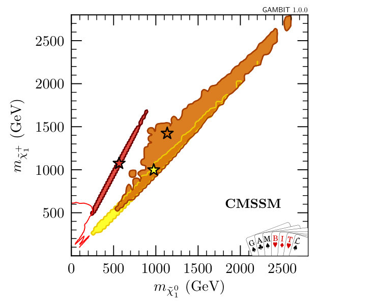 Figure 1
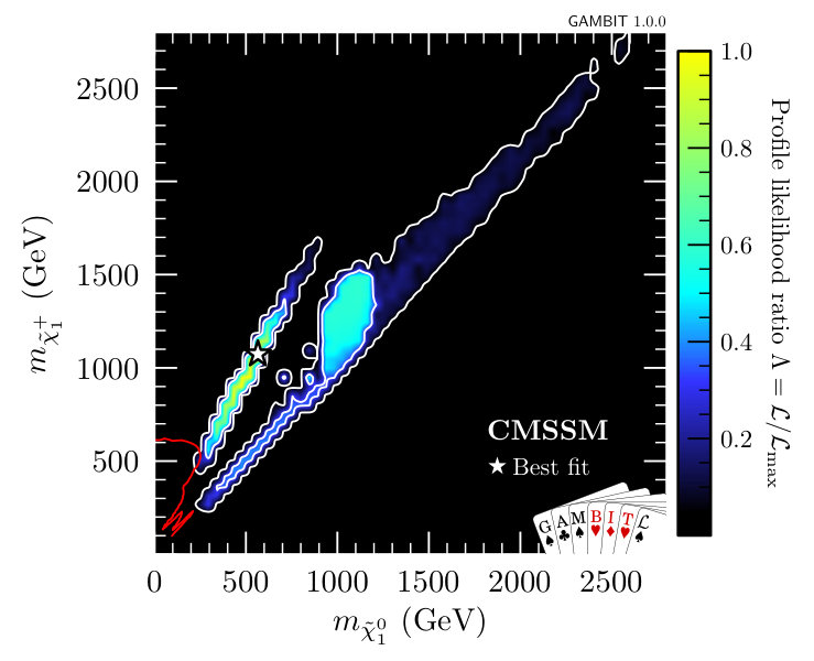 Figure 2
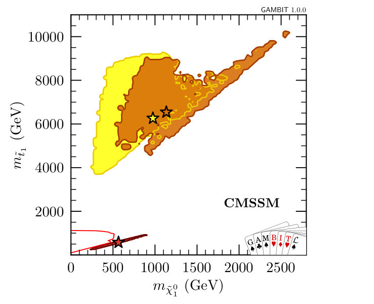 Figure 3
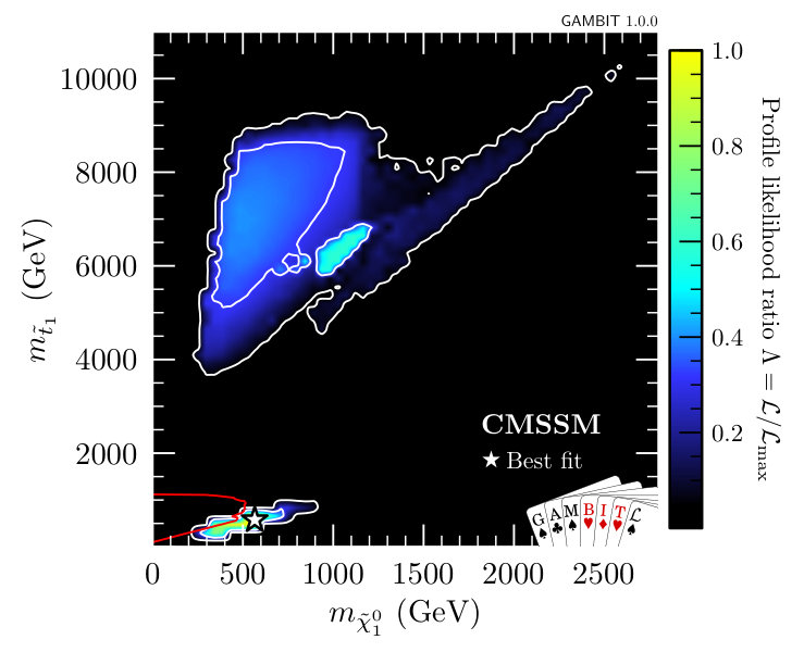 Figure 4
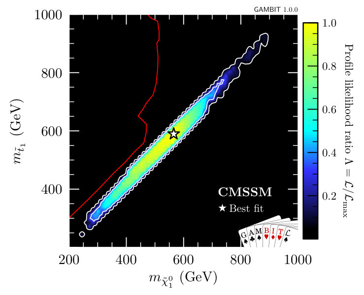 Figure 5
 Figure 6
 Figure 7
 Figure 8
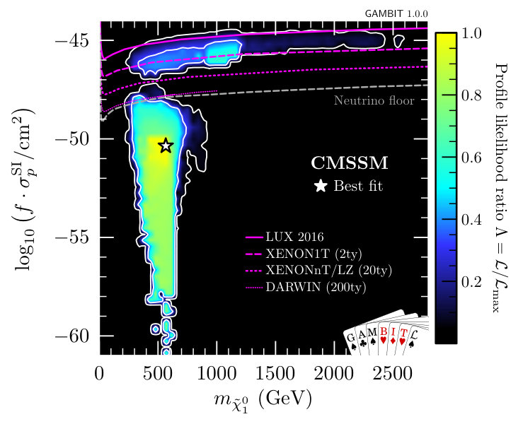 Figure 9
 Figure 10
 Figure 11
 Figure 12
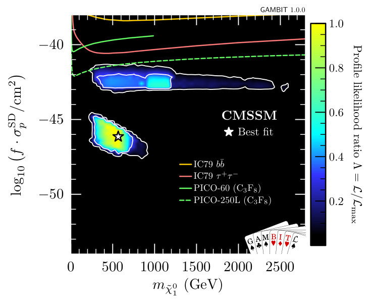 Figure 13
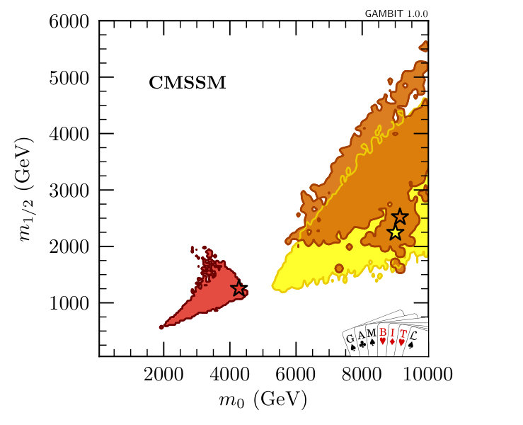 Figure 14
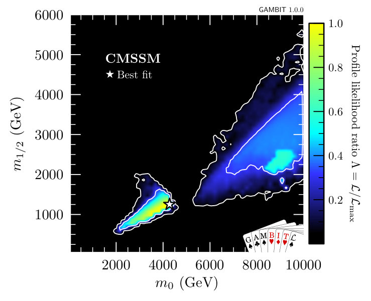 Figure 15
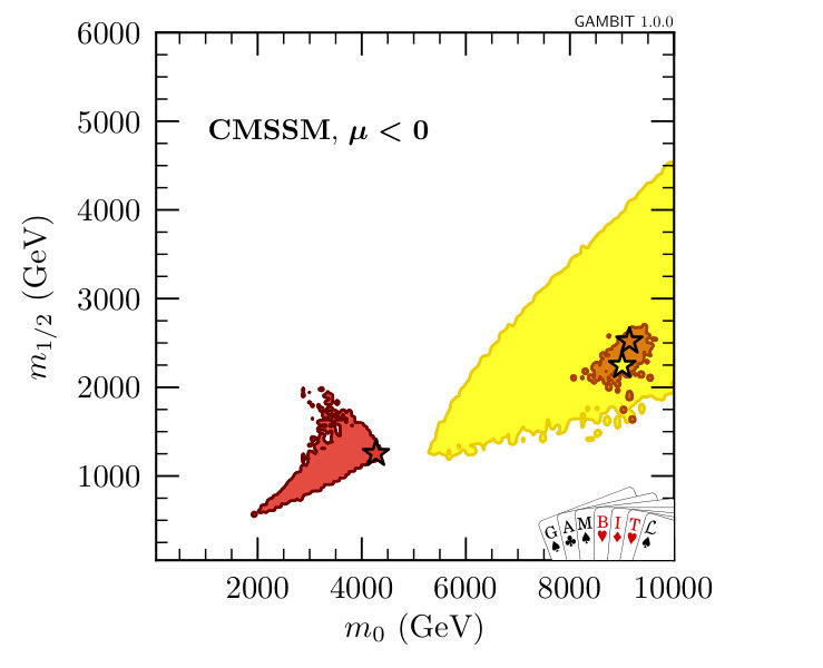 Figure 16
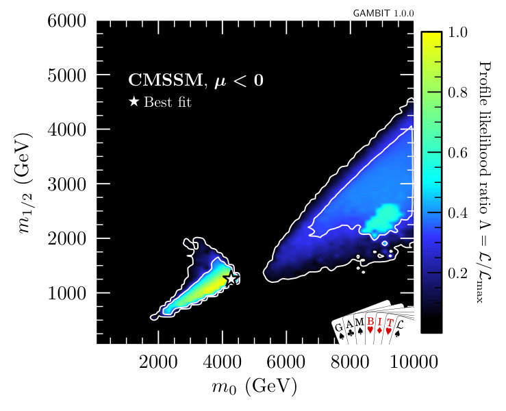 Figure 17
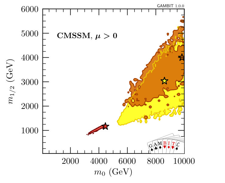 Figure 18
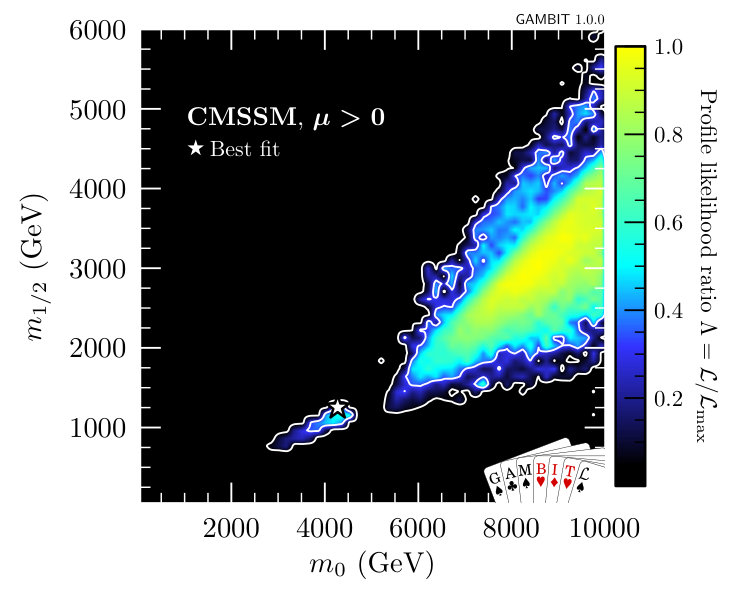 Figure 19
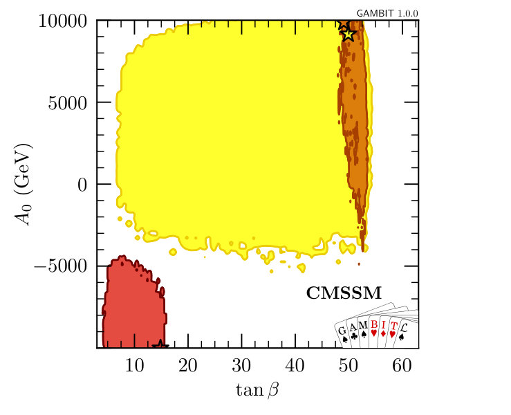 Figure 20
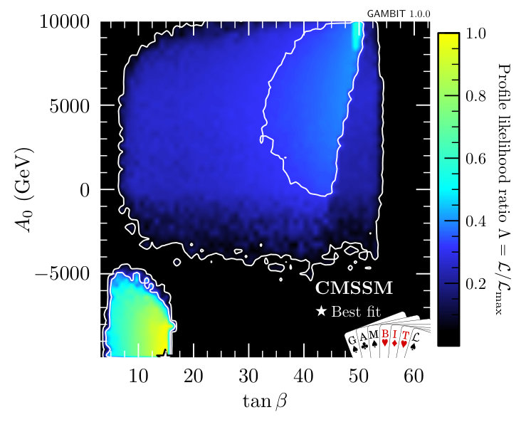 Figure 21
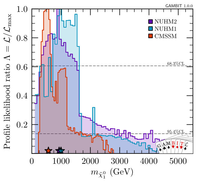 Figure 22
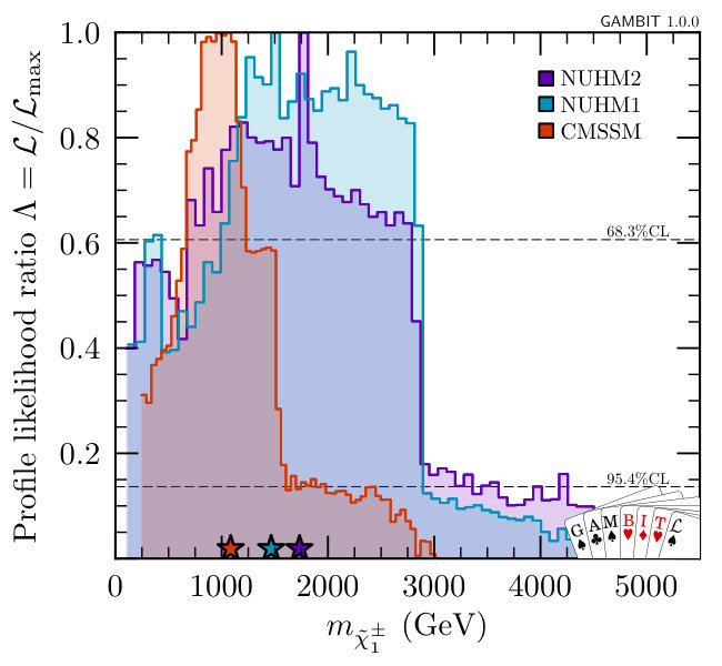 Figure 23
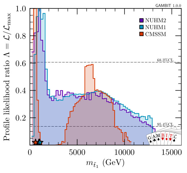 Figure 24
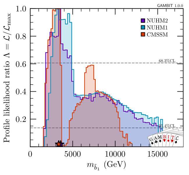 Figure 25
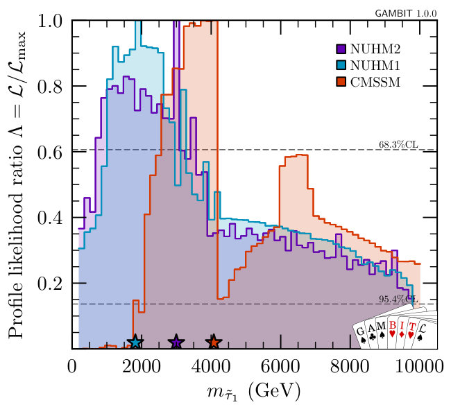 Figure 26
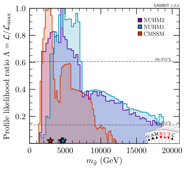 Figure 27
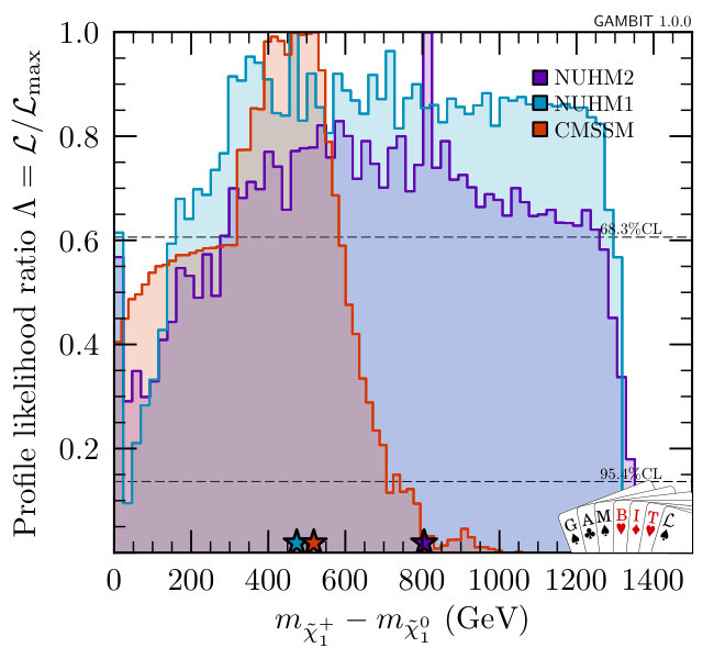 Figure 28
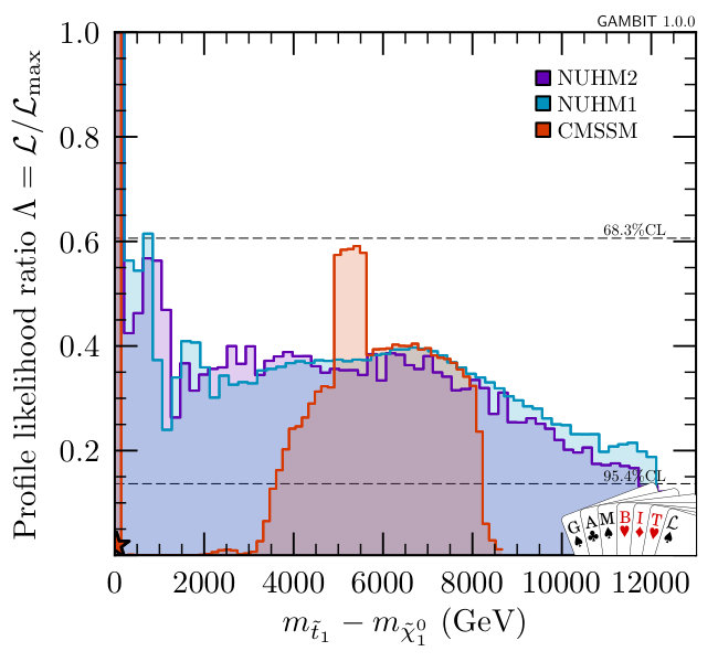 Figure 29
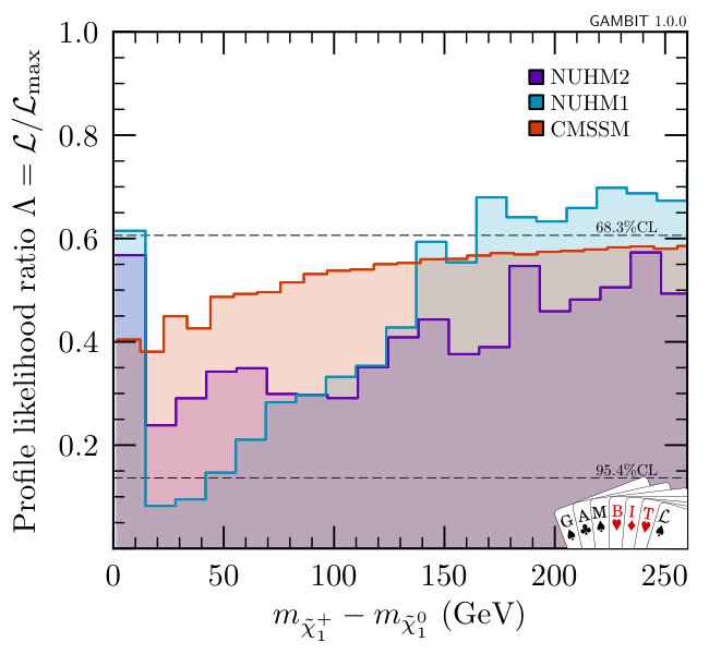 Figure 30
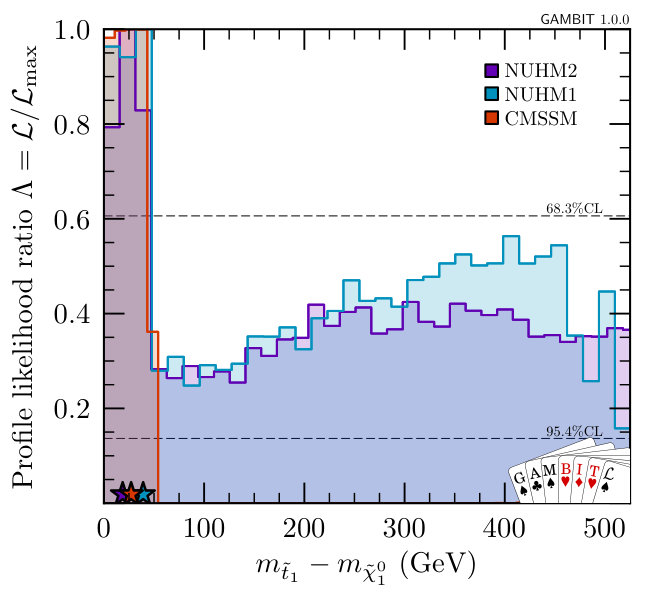 Figure 31
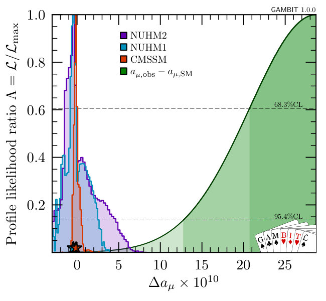 Figure 32
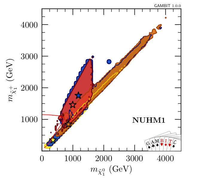 Figure 33
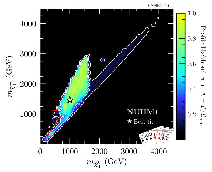 Figure 34
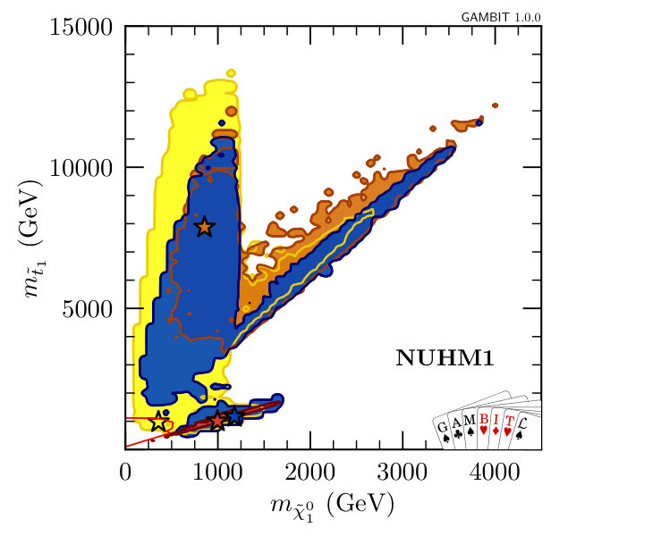 Figure 35
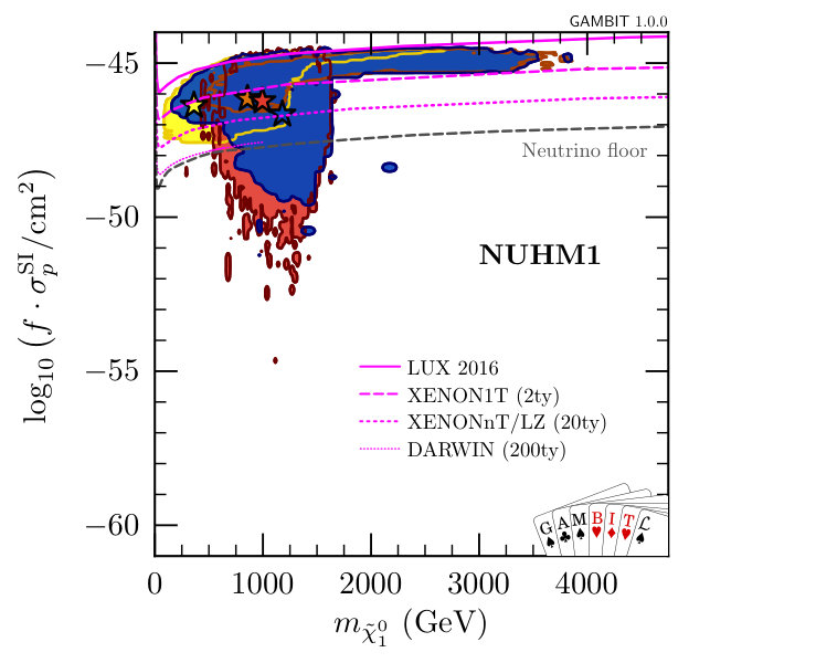 Figure 36
 Figure 37
 Figure 38
 Figure 39
 Figure 40
| Parameter | Minimum | Maximum | Priors |
|---|---|---|---|
| CMSSM | |||
| 50 GeV | 10 TeV | flat, log | |
| 50 GeV | 10 TeV | flat, log | |
| 10 TeV | 10 TeV | flat, hybrid | |
| 3 | 70 | flat | |
| binary | |||
| NUHM1 – as per CMSSM plus | |||
| 50 GeV | 10 TeV | flat, log | |
| NUHM2 – as per CMSSM plus | |||
| 50 GeV | 10 TeV | flat, log | |
| 50 GeV | 10 TeV | flat, log | |
| Parameter | Value(Range) | |
| Varied | ||
| Strong coupling | ||
| Top quark pole mass | GeV | |
| Local DM density | 0.2–0.8 GeV cm-3 | |
| Nuclear matrix el. (strange) | MeV | |
| Nuclear matrix el. (up + down) | MeV | |
| Fixed | ||
| Electromagnetic coupling | ||
| Fermi coupling | ||
| Z pole mass | GeV | |
| Bottom quark mass | GeV | |
| Charm quark mass | GeV | |
| Strange quark mass | MeV | |
| Down quark mass | MeV | |
| Up quark mass | MeV | |
| pole mass | GeV | |
| CKM Wolfenstein parameters: | 0.22537 | |
| 0.814 | ||
| 0.117 | ||
| 0.353 | ||
| Most probable halo speed | 235 km s-1 | |
| Local disk circular velocity | 235 km s-1 | |
| Local escape velocity | 550 km s-1 | |
| Up contribution to proton spin | 0.842 | |
| Down contrib. to proton spin | 0.427 | |
| Strange contrib. to proton spin | 0.085 |
| Scanner | Parameter | Setting |
|---|---|---|
| Diver | NP | 19 200 |
| convthresh | ||
| Diver | NP | 6000 |
| (co-annihilation) | convthresh | |
| MultiNest | nlive | 5000 |
| tol | 0.1 |
| Production | Decay | Experiment |
|---|---|---|
| +c.c. | ALEPH Heister:2001nk , L3 L3:sleptons_squarks | |
| OPAL OPAL:gauginos | ||
| () | L3 L3:gauginos | |
| OPAL OPAL:gauginos | ||
| () | OPAL OPAL:gauginos | |
| OPAL OPAL:gauginos , L3 L3:gauginos |
| Likelihood term | Ideal | -funnel | co-ann. | co-ann. | co-ann. | |
|---|---|---|---|---|---|---|
| LHC sparticle searches | ||||||
| LHC Higgs | ||||||
| LEP Higgs | ||||||
| ALEPH selectron | ||||||
| ALEPH smuon | ||||||
| ALEPH stau | ||||||
| L3 selectron | ||||||
| L3 smuon | ||||||
| L3 stau | ||||||
| L3 neutralino leptonic | ||||||
| L3 chargino leptonic | ||||||
| OPAL chargino hadronic | ||||||
| OPAL chargino semi-leptonic | ||||||
| OPAL chargino leptonic | ||||||
| OPAL neutralino hadronic | ||||||
| Tree-level and decays | ||||||
| mass | ||||||
| Relic density | ||||||
| PICO-2L | ||||||
| PICO-60 F | ||||||
| SIMPLE 2014 | ||||||
| LUX 2015 | ||||||
| LUX 2016 | ||||||
| PandaX 2016 | ||||||
| SuperCDMS 2014 | ||||||
| XENON100 2012 | ||||||
| IceCube 79-string | ||||||
| rays (Fermi-LAT dwarfs) | ||||||
| and | ||||||
| Top quark mass | ||||||
| Total | ||||||
| Quantity | -funnel | co-ann. | co-ann. | co-ann. | ||
| %bino, %Higgsino | ||||||
| %bino, %Higgsino | ||||||
| %wino, %Higgsino | ||||||
Peer Reviews
No public reviews on file for this paper yet. If you reviewed it on a platform where reviews are public (OpenReview, ICLR, NeurIPS, ICML), you can paste yours below so the community can read it here.
Videos
No videos yet. Explain this paper in a talk, walkthrough, or lecture? Add one.
∎
\lst@KeylabelnameListing
language=C++, basicstyle=, basewidth=0.53em,0.44em, numbers=none, tabsize=2, breaklines=true, escapeinside=@@, showstringspaces=false, numberstyle=, keywordstyle=, stringstyle=, identifierstyle=, commentstyle=, directivestyle=, emphstyle=, frame=single, rulecolor=, rulesepcolor=, literate=
1, moredelim=[directive] #, moredelim=[directive] #
language=C++, basicstyle=, basewidth=0.53em,0.44em, numbers=none, tabsize=2, breaklines=true, escapeinside=@@, showstringspaces=false, numberstyle=, keywordstyle=, stringstyle=, identifierstyle=, commentstyle=, directivestyle=, emphstyle=, frame=single, rulecolor=, rulesepcolor=, literate=
1, moredelim=**[is][#define]BeginLongMacroEndLongMacro
language=C++, basicstyle=, basewidth=0.53em,0.44em, numbers=none, tabsize=2, breaklines=true, escapeinside=@@, numberstyle=, showstringspaces=false, numberstyle=, keywordstyle=, stringstyle=, identifierstyle=, commentstyle=, directivestyle=, emphstyle=, frame=single, rulecolor=, rulesepcolor=, literate=
1, moredelim=[directive] #, moredelim=[directive] #
language=Python, basicstyle=, basewidth=0.53em,0.44em, numbers=none, tabsize=2, breaklines=true, escapeinside=@@, showstringspaces=false, numberstyle=, keywordstyle=, stringstyle=, identifierstyle=, commentstyle=, emphstyle=, frame=single, rulecolor=, rulesepcolor=, literate =
1 as as 3
language=Fortran, basicstyle=, basewidth=0.53em,0.44em, numbers=none, tabsize=2, breaklines=true, escapeinside=@@, showstringspaces=false, numberstyle=, keywordstyle=, stringstyle=, identifierstyle=, commentstyle=, emphstyle=, morekeywords=and, or, true, false, frame=single, rulecolor=, rulesepcolor=, literate=
1
language=bash, basicstyle=, numbers=none, tabsize=2, breaklines=true, escapeinside=@@, frame=single, showstringspaces=false, numberstyle=, keywordstyle=, stringstyle=, identifierstyle=, commentstyle=, emphstyle=, frame=single, rulecolor=, rulesepcolor=, morekeywords=gambit, cmake, make, mkdir, deletekeywords=test, literate = gambit gambit7 /gambit/gambit6 gambit/gambit/6 /include/include8 cmake/cmake/6 .cmake.cmake6
1
language=, basicstyle=, identifierstyle=, numbers=none, tabsize=2, breaklines=true, escapeinside=@@, showstringspaces=false, frame=single, rulecolor=, rulesepcolor=, literate=
1
language=bash, escapeinside=@@, keywords=true,false,null, otherkeywords=, keywordstyle=, basicstyle=, identifierstyle=, sensitive=false, commentstyle=, morecomment=[l]#, morecomment=[s]//, stringstyle=, moredelim=[s][],:, moredelim=[l][]:, morestring=[b]’, morestring=[b]", literate = ------3
1 ||1 - - 3 } }1 { {1 [ [1 ] ]1
1, breakindent=0pt, breakatwhitespace, columns=fullflexible **
language=Mathematica, basicstyle=, basewidth=0.53em,0.44em, numbers=none, tabsize=2, breaklines=true, escapeinside=@@, numberstyle=, showstringspaces=false, numberstyle=, keywordstyle=, stringstyle=, identifierstyle=, commentstyle=, directivestyle=, emphstyle=, frame=single, rulecolor=, rulesepcolor=, literate=
1, moredelim=[directive] #, moredelim=[directive] #, mathescape=true
11institutetext: School of Physics and Astronomy, Monash University, Melbourne, VIC 3800, Australia 22institutetext: Australian Research Council Centre of Excellence for Particle Physics at the Tera-scale 33institutetext: Department of Physics, University of Oslo, N-0316 Oslo, Norway 44institutetext: SUPA, School of Physics and Astronomy, University of Glasgow, Glasgow, G12 8QQ, UK 55institutetext: Physik-Institut, Universität Zürich, Winterthurerstrasse 190, 8057 Zürich, Switzerland 66institutetext: H. Niewodniczański Institute of Nuclear Physics, Polish Academy of Sciences, 31-342 Kraków, Poland 77institutetext: Oskar Klein Centre for Cosmoparticle Physics, AlbaNova University Centre, SE-10691 Stockholm, Sweden 88institutetext: Department of Physics, Stockholm University, SE-10691 Stockholm, Sweden 99institutetext: Department of Physics, McGill University, 3600 rue University, Montréal, Québec H3A 2T8, Canada 1010institutetext: Department of Physics, University of Adelaide, Adelaide, SA 5005, Australia 1111institutetext: NORDITA, Roslagstullsbacken 23, SE-10691 Stockholm, Sweden 1212institutetext: Univ Lyon, Univ Lyon 1, ENS de Lyon, CNRS, Centre de Recherche Astrophysique de Lyon UMR5574, F-69230 Saint-Genis-Laval, France 1313institutetext: Theoretical Physics Department, CERN, CH-1211 Geneva 23, Switzerland 1414institutetext: Physics and Astronomy Department, University of California, Los Angeles, CA 90095, USA 1515institutetext: LAPTh, Université de Savoie, CNRS, 9 chemin de Bellevue B.P.110, F-74941 Annecy-le-Vieux, France 1616institutetext: Department of Physics, Harvard University, Cambridge, MA 02138, USA 1717institutetext: Instituto de Física Corpuscular, IFIC-UV/CSIC, Valencia, Spain 1818institutetext: Centre for Translational Data Science, Faculty of Engineering and Information Technologies, School of Physics, The University of Sydney, NSW 2006, Australia 1919institutetext: Department of Physics, Imperial College London, Blackett Laboratory, Prince Consort Road, London SW7 2AZ, UK 2020institutetext: GRAPPA, Institute of Physics, University of Amsterdam, Science Park 904, 1098 XH Amsterdam, Netherlands
\thankstext
[email protected] \[email protected] \[email protected] \[email protected] \[email protected] \thankstext[*]e6Also Institut Universitaire de France, 103 boulevard Saint-Michel, 75005 Paris, France.
Global fits of GUT-scale SUSY models with GAMBIT
The GAMBIT Collaboration: Peter Athron\thanksrefinst:a,inst:b,e1
Csaba Balázs\thanksrefinst:a,inst:b
Torsten Bringmann\thanksrefinst:c
Andy Buckley\thanksrefinst:d
Marcin Chrząszcz\thanksrefinst:e,inst:f
Jan Conrad\thanksrefinst:g,inst:h
Jonathan M. Cornell\thanksrefinst:i
Lars A. Dal\thanksrefinst:c
Joakim Edsjö\thanksrefinst:g,inst:h
Ben Farmer\thanksrefinst:g,inst:h,e2
Paul Jackson\thanksrefinst:k,inst:b
Abram Krislock\thanksrefinst:c
Anders Kvellestad\thanksrefinst:m,e3
Farvah Mahmoudi\thanksrefinst:n,inst:o,e6
Gregory D. Martinez\thanksrefinst:p
Antje Putze\thanksrefinst:r
Are Raklev\thanksrefinst:c
Christopher Rogan\thanksrefinst:s
Roberto Ruiz de Austri\thanksrefinst:v
Aldo Saavedra\thanksrefinst:t,inst:b
Christopher Savage\thanksrefinst:m
Pat Scott\thanksrefinst:q,e4
Nicola Serra\thanksrefinst:e
Christoph Weniger\thanksrefinst:u
Martin White\thanksrefinst:k,inst:b,e5
(Received: date / Accepted: date)
Abstract
We present the most comprehensive global fits to date of three supersymmetric models motivated by grand unification: the Constrained Minimal Supersymmetric Standard Model (CMSSM), and its Non-Universal Higgs Mass generalisations NUHM1 and NUHM2. We include likelihoods from a number of direct and indirect dark matter searches, a large collection of electroweak precision and flavour observables, direct searches for supersymmetry at LEP and Runs I and II of the LHC, and constraints from Higgs observables. Our analysis improves on existing results not only in terms of the number of included observables, but also in the level of detail with which we treat them, our sampling techniques for scanning the parameter space, and our treatment of nuisance parameters. We show that stau co-annihilation is now ruled out in the CMSSM at more than 95% confidence. Stop co-annihilation turns out to be one of the most promising mechanisms for achieving an appropriate relic density of dark matter in all three models, whilst avoiding all other constraints. We find high-likelihood regions of parameter space featuring light stops and charginos, making them potentially detectable in the near future at the LHC. We also show that tonne-scale direct detection will play a largely complementary role, probing large parts of the remaining viable parameter space, including essentially all models with multi-TeV neutralinos.
††journal: Eur. Phys. J. C
Contents
1 Introduction
Although the Standard Model (SM) of particle physics has long provided a spectacularly successful description of physics at and below the electroweak scale, it remains incomplete. Explaining dark matter (DM), the asymmetry between matter and antimatter, the hierarchy between the Planck and electroweak scales, the origin of the fundamental forces and charges, or anomalies in low-energy precision and flavour measurements, requires extending the SM by adding one or more new particles.
The Minimal Supersymmetric extension of the SM (MSSM) offers solutions to many of these shortcomings, with substantial implications for dark matter Profumo:2016zxo ; Roy:2016zst ; arXiv:1602.08103 ; arXiv:1602.01030 ; arXiv:1602.00590 ; arXiv:1601.04718 ; IC79_SUSY ; arXiv:1511.05964 ; arXiv:1511.05386 ; arXiv:1510.07616 ; arXiv:1510.07501 ; arXiv:1510.06295 ; arXiv:1510.05378 ; arXiv:1510.04291 ; arXiv:1510.03498 ; arXiv:1510.03460 ; arXiv:1510.02470 ; arXiv:1510.02473 ; arXiv:1509.09159 ; arXiv:1509.05076 ; arXiv:1508.04383 ; arXiv:1508.04373 ; arXiv:1507.06164 ; arXiv:1412.4789 ; arXiv:1507.05584 ; arXiv:1507.04644 ; arXiv:1505.04595 ; Crivellin:2015oha ; arXiv:1504.05554 ; arXiv:1504.05091 ; arXiv:1504.00915 ; arXiv:1504.00504 ; arXiv:1503.07142 ; arXiv:1503.03478 ; arXiv:1503.00599 ; arXiv:1502.06000 ; arXiv:1502.05703 ; arXiv:1502.05672 ; arXiv:1502.05406 ; arXiv:1412.8698 , the cosmic matter-antimatter asymmetry arXiv:1512.09172 ; arXiv:1508.04144 ; arXiv:1508.00011 , Higgs physics Athron:2016fuq ; arXiv:1608.02573 ; Bahl:2016brp ; arXiv:1608.00638 ; arXiv:1601.01890 ; arXiv:1512.00437 ; arXiv:1511.08461 ; arXiv:1511.07853 ; arXiv:1511.06002 ; arXiv:1507.04469 ; arXiv:1506.08462 ; arXiv:1505.01059 ; arXiv:1504.06932 ; arXiv:1504.06625 ; arXiv:1504.05200 ; arXiv:1504.04308 ; arXiv:1502.05653 , the unification of gauge forces arXiv:1702.05431 ; arXiv:1611.08341 ; arXiv:1610.10084 ; Ellis:2016tjc ; arXiv:1512.09148 ; arXiv:1511.06205 ; arXiv:1509.08838 ; arXiv:1508.04176 ; arXiv:1506.05962 ; arXiv:1506.05850 ; arXiv:1505.04950 ; arXiv:1504.00904 ; arXiv:1504.00505 ; arXiv:1501.05307 ; arXiv:1501.02906 ; arXiv:1412.5766 , the stability of the electroweak vacuum arXiv:1606.08356 ; Bagnaschi:2015pwa ; Blinov:2013fta ; Carena:2012mw , cosmological inflation Ferrara:2016vzg ; arXiv:1503.08867 ; arXiv:1407.4110 ; arXiv:1405.4125 ; arXiv:1312.3623 ; arXiv:1309.7788 ; arXiv:1305.1066 ; arXiv:1304.5202 ; arXiv:1303.5351 ; arXiv:1205.2815 , precision measurements Kobakhidze:2016mdx ; gm2calc ; arXiv:1510.04263 ; arXiv:1507.05836 ; arXiv:1505.01987 ; arXiv:1504.05500 ; arXiv:1503.08703 ; arXiv:1503.08219 ; arXiv:1503.06850 and flavor physics arXiv:1509.05414 ; arXiv:1504.00930 ; arXiv:1501.02044 .
Even though the MSSM framework is predictive, its Lagrangian terms responsible for softly breaking SUSY contain over a hundred new parameters. This impairs the practical predictivity of the model. Mediation of supersymmetry breaking by Planck-scale physics is a popular and viable motivation for reducing the free parameters to a small number at the Grand Unified Theory (GUT) scale Chamseddine:1982jx ; Barbieri:1982eh ; Ibanez:1982ee ; Hall:1983iz ; Ellis:1982wr ; AlvarezGaume:1983gj . Here we analyse three scenarios motivated by gravity mediation: the Constrained MSSM (CMSSM) Nilles:1983ge and two of its Non-Universal Higgs Mass (NUHM1, NUHM2) extensions Matalliotakis:1994ft ; Olechowski:1994gm ; Berezinsky:1995cj ; Drees:1996pk ; Nath:1997qm .
Opinions differ regarding the phenomenological feasibility of these models, especially the CMSSM. Global fits of the CMSSM after Run I of the Large Hadron Collider (LHC) indicate that its experimentally-viable parameter space has been pushed to regions with superpartners heavier than 1 TeV. The relic density of DM in these scenarios is set by neutralino-stau co-annihilation, resonant annihilation through a heavy Higgs, or a large Higgsino component Han:2016gvr ; Bechtle:2014yna ; arXiv:1405.4289 ; arXiv:1402.5419 ; MastercodeCMSSM ; arXiv:1312.5233 ; arXiv:1310.3045 ; arXiv:1309.6958 ; arXiv:1307.3383 ; arXiv:1304.5526 ; arXiv:1212.2886 ; Strege13 ; Gladyshev:2012xq ; Kowalska:2012gs ; MasterCode12b ; arXiv:1207.1839 ; arXiv:1207.4846 ; Roszkowski12 ; SuperbayesHiggs ; Fittino12 ; MasterCode12 ; arXiv:1111.6098 ; Fittino ; Trotta08 ; Ruiz06 ; Allanach06 ; Fittino06 ; Baltz04 ; SFitter . Relaxing the assumption of scalar soft-mass universality at the GUT scale provides much more flexible phenomenology arXiv:1509.02929 ; Mastercode15 ; arXiv:1502.04127 ; arXiv:1412.3403 ; Buchmueller:2014yva ; arXiv:1407.1481 ; arXiv:1404.2277 ; arXiv:1312.5233 ; arXiv:1309.2984 ; arXiv:1309.0036 ; arXiv:1307.0782 ; arXiv:1306.0344 ; Fittino12 . Global fits of the NUHM1 show that the tension that exists in the CMSSM between the measured Higgs mass and precision/flavour observables is reduced due to the decoupling of the Higgs sector from the squark and slepton sectors, and a new region of chargino co-annihilation opens up for dark matter Mastercode15 ; Buchmueller:2014yva ; arXiv:1405.4289 ; MastercodeCMSSM ; arXiv:1312.5233 ; Strege13 ; Fittino12 . Extending the parameter space to the NUHM2 Mastercode15 ; Buchmueller:2014yva ; arXiv:1405.4289 relaxes the constraints on the scalar masses even further.
In this work we use the GAMBIT framework gambit ; DarkBit ; ColliderBit ; FlavBit ; SDPBit ; ScannerBit to scan and assess the viability of the parameter spaces of each of these three GUT-scale scenarios in detail. We also carry out a detailed comparison of our results with previous ones, to understand the impact of the improved theoretical calculations and updated experimental data that we include, and as a verification of our new computational framework. We have also carried out similar analyses of scalar singlet DM SSDM and ‘phenomenological’ (weak-scale) SUSY models MSSM with the GAMBIT framework.
There are several important features of our study that make it the most definitive exploration of the CMSSM, NUHM1 or NUHM2 to date:
We apply the DM relic density constraint as an upper bound only. This requires that the cosmological density of the lightest neutralino does not exceed the observed density of DM. This is a conservative option from the point of view of excluding a light mass spectrum, as it introduces more possibilities for light Higgsino and light Higgsino-bino DM than in studies where a lower bound is also applied. 2. 2.
We include a significantly higher number of observables in our combined likelihood than has been done before. These include rates in multiple direct and indirect searches for DM, a wide range of LHC sparticle searches and Higgs observables, and an up-to-date set of flavour physics observables and electroweak precision measurements. 3. 3.
In addition to improving the quantity of data included in the fit, we have also improved the quality of the typical simulation treatments, including direct Monte Carlo simulation of LHC observables during the global fit, event-level indirect search likelihoods, and direct DM search limits based on rigorous simulation of the relevant experiments. 4. 4.
Using GAMBIT allows us to pursue a thorough theoretical and statistical approach, where theoretical assumptions are consistently treated across different observables and experimental searches. This includes the accurate treatment, via nuisance parameters, of uncertainties associated with the local DM distribution, nuclear matrix elements relevant for direct detection, and SM parameters. 5. 5.
GAMBIT includes an interface to Diver ScannerBit , a new scanner based on differential evolution, which provides significantly improved sampling performance compared to conventional techniques. This allows us to more accurately locate and more comprehensively map small regions of high likelihood. 6. 6.
The public, open-source nature of GAMBIT 111gambit.hepforge.org makes our study transparent, reproducible and extendible by the reader.
In Section 2, we introduce the CMSSM, NUHM1 and NUHM2, along with their parameters, the ranges and priors over which we vary those parameters, and the algorithms and settings that we use for sampling them. Section 3 contains a summary of the experimental data, observables and likelihood calculations that go into each fit. We then present our results in Section 4, before looking at the implications of our scans for future searches for the models in question, and concluding in Section 5.
All input files, samples and best-fit benchmarks produced for this paper are publicly accessible from Zenodo the_gambit_collaboration_2017_801642 .
2 Models and scanning framework
2.1 Model definitions and parameters
From a statistical standpoint, there is no fundamental difference between models that describe SM physics (and astrophysics) and physics beyond the SM (BSM). GAMBIT therefore treats BSM models on exactly the same footing as models that describe nuisance parameters, which are designed to quantify uncertainties on better-constrained quantities. The only difference is that nuisance models are generally more strongly constrained by the likelihood than BSM models.
In this paper, we simultaneously sample from four models in each scan: one GUT-scale SUSY model (CMSSM, NUHM1 or NUHM2; Sec. 2.1.1), and three specific nuisance models. The first nuisance model includes the parameters of the SM (Sec. 2.1.2), the second parameterises the density and velocity distribution of the DM halo (Sec. 2.1.3), and the third encapsulates the nuclear uncertainties relevant for DM direct detection (Sec. 2.1.4).
2.1.1 SUSY models
The definitions of the MSSM superpotential and soft-breaking Lagrangian that we use are specified in Sec. 5.4.3 of Ref. gambit , and we follow the conventions established there. All the BSM models that we investigate in this paper are subsets of the GAMBIT model MSSM63atMGUT gambit , which is the most general formulation of the -conserving MSSM, with the soft masses defined at the scale where the gauge couplings and unify (the GUT scale).
The complexity of the MSSM can be reduced considerably if one makes simplifying assumptions about the values of the soft masses at the GUT scale:
CMSSM
The soft mass parameters at the GUT scale are fixed to a universal scalar mass , a universal gaugino mass and a universal trilinear coupling . The diagonal elements in the sfermion mass-squared matrices , , , and are set to , all off-diagonal elements are set to zero, and the scalar Higgs mass-squared parameters and are set to . The gaugino masses , and are set to and all trilinear couplings, and are set to . Electroweak symmetry breaking (EWSB) conditions fix the soft-breaking bilinear and the magnitude of the superpotential bilinear at the SUSY scale. The remaining free parameters in the Higgs sector are the sign of and the ratio of the vacuum expectation values of the two Higgs doublets , which is defined at the scale . The CMSSM is defined by , , , , and .
NUHM1
The GUT-scale constraint on the soft scalar Higgs masses is relaxed, introducing the additional free parameter . The soft Higgs masses and are not set equal to , but instead obey the relation at the GUT scale. Here is treated as a real dimension-one parameter, ignoring scenarios where . This means that at the GUT scale we require , which acts as the boundary condition under which the correct shape of the Higgs potential must be radiatively generated at the electroweak scale. The parameters of the NUHM1 are , , , , and .
NUHM2
The constraint on the soft Higgs masses is further relaxed so that and become independent, real, dimension-one parameters at the GUT scale. As in the NUHM1, and are always positive at the GUT scale, and the correct shape of the Higgs potential at the electroweak scale must be radiatively generated. The parameters are thus , , , , , and .
We assume throughout that -parity is conserved, making the lightest supersymmetric particle (LSP) stable. In this paper we consider only the possibility of neutralino LSPs, assigning zero likelihood to all parameter combinations where this is not the case. Sneutrino DM in the MSSM Falk:1994es is now essentially ruled out by direct detection, though it remains viable in MSSM extensions (see Ref. Arina:2007tm for a review). Gravitino LSP scenarios (e.g. Roszkowski:2004jd ; Arvey:2015nra ) are still viable even in the CMSSM, so adding such models to the results that we present here would be an interesting future extension.
The parameter ranges that we scan over for the CMSSM, NUHM1 and NUHM2 can be found in Table 1. We allow the magnitudes of all dimensionful parameters to vary between 50 GeV and 10 TeV. The lower cutoff is motivated by the constraints on sparticle masses from existing searches. The upper cutoff is somewhat arbitrary, but designed to encompass the mass range interesting for solving the hierarchy problem, and for leading to potentially-observable phenomenology. We consider both positive and negative , and the full range of over which particle spectra can be consistently calculated and EWSB achieved in such models.
2.1.2 Standard Model
Here we define the SM as per SLHA2 Allanach:2008qq , sampling from the GAMBIT model StandardModel_SLHA2 gambit . We identify the strength of the strong coupling at the scale of the mass, , and the top quark pole mass, , as the most relevant nuisance parameters within this model. Both affect the running of soft-breaking masses from the GUT scale. The mass of the SM-like Higgs boson is also very sensitive to the top quark mass, and has a strong influence on the scan through the Higgs likelihood (see Sec. 3.11).
In all our fits, we allow both these parameters to vary within of their observed central values ATLAS:2014wva ; PDB . The resulting parameter ranges are shown in Table 2. We adopt flat priors on both and ; their values are sufficiently well-determined that the prior has no impact on results. The values of other SM parameters that we keep fixed in our scans are also shown in Table 2.
2.1.3 Dark matter halo model
The density and velocity distributions that characterise the DM halo of the Milky Way constitute an important source of uncertainty for astrophysical observations, particularly direct and indirect searches for DM. In this paper, we employ the GAMBIT model Halo_gNFW_rho0 gambit to describe the halo. This consists of a generalised NFW Navarro:1995iw spatial profile, tied to a locally Maxwell-Boltzmann velocity distribution by a specific input local density .
Because we do not employ any observables in our fits that depend on the Milky Way density profile, the spatial part of this model plays no role. The local distribution of DM velocities is given by
[TABLE]
where is the local Galactic escape velocity, is the most probable particle speed and
[TABLE]
is the normalisation factor induced by truncating the distribution at .
In the Earth’s rest frame, DM particles have a velocity distribution given by:
[TABLE]
where is the velocity of the Earth relative to the Milky Way DM halo. This is given by:
[TABLE]
where km s*-1* is the peculiar velocity of the Sun, which is known with very high precision Schoenrich:2009bx . The Local Standard of Rest (LSR) in Galactic coordinates moves with a velocity , while km s*-1* Freese:2012xd denotes the speed of the Earth in the solar rest frame.
For an NFW profile is within 10% of . As shown in Table 2, we set both these parameters to 235 km s*-1* DarkBit ; Reid:2009nj ; Bovy:2009dr in all our scans. Similarly, we adopt a fixed value of 550 km s*-1* for the local escape speed Smith:2006ym .
Because it has a substantial impact on direct detection and high-energy solar neutrino signals from DM, we vary the local density of DM as a nuisance parameter in all scans (Table 2). Here we adopt an asymmetric range of GeV cm*-3* around the canonical value of GeV cm*-3*, reflecting the log-normal form of the likelihood that we apply to this parameter (see Sec. 3.1.2). The prior on has no impact because it is sufficiently well-constrained by the associated nuisance likelihood; we choose to make it flat.
See Refs. DarkBit ; Akrami:2010dn for further discussion and details of the DM halo model, parameters and uncertainties.
2.1.4 Nuclear model
A final class of uncertainty relevant for direct detection and neutralino capture by the Sun is due to the effective nuclear couplings in WIMP-nucleon cross-sections. For spin-independent interactions, these depend on the light-quark composition of the proton and the neutron. We scan the GAMBIT model nuclear_params_sigmas_sigmal, parameterising the 6 individual hadronic matrix elements in terms of just two nuclear matrix elements
[TABLE]
which we take to be identical for and Young:2013nn . These two parameters, respectively, describe the light-quark and strange-quark contents of the nucleus. We vary and over their ranges in all fits. Discussion of the values and uncertainties of these parameters can be found in Sec. 3.1.3 and the DarkBit paper DarkBit . Like all other nuisance parameters listed in Table 2, the nuclear matrix elements are sufficiently well constrained that the prior is irrelevant, so we choose it to be flat.
The spin-dependent couplings are described by the spin content of the proton and neutron for each light quark . As the values for the proton and neutron are related, only three of these parameters are independent. As listed in Table 2, we specify the values for the proton, and set them to the central values discussed in Ref. DarkBit .
2.2 Scanning methodology
In this paper we carry out a number of different scans of each of the three GUT-scale models, employing multiple priors, sampling algorithms and settings. We then merge the results of all scans for each model, in order to obtain the most complete sampling of the profile likelihood possible. We leave discussion and presentation of Bayesian posteriors for a future paper, as they remain strongly dominated by the choice of prior even in such low-dimensional versions of the MSSM, and a detailed analysis of the their implications for fine-tuning and naturalness (e.g. Allanach:2007qk ; Cabrera:2008tj ) is beyond the scope of the current paper.
The parameter ranges and priors that we employ in scans of each model are listed in Table 1. We repeat every scan for positive and negative values of . We carry out scans with both flat and logarithmic priors on all dimensionful parameters. In the case of the trilinear coupling , which may be positive or negative, in our log-prior scans we employ a hybrid prior (log_flat_join in the language of Ref. ScannerBit ), consisting of a symmetric logarithmic prior at large , truncated to a flat prior at GeV.
We use two different samplers for our scans: Diver 1.0.0 ScannerBit and MultiNest 3.10 MultiNest . The settings that we use for each can be found in Table 3.
Diver is a self-adaptive sampler based on differential evolution StornPrice95 . It samples the profile likelihood far more efficiently than traditional algorithms ScannerBit , allowing high-quality profile likelihoods to be computed in a fraction of the time of previous SUSY global fits, using significantly fewer likelihood samples. As a result, the majority of our results are driven by the Diver scans. Following the extensive tests discussed in Ref. ScannerBit , for most scans222For the special case of flat-prior CMSSM scans, where less stringent parameters already provide quite sufficient sampling, we use NP = 14 400, convthresh = 10*-4*. we choose a population size of NP = 19 200 and a convergence threshold of convthresh = 10*-5*. The latter is defined in terms of the smoothed fractional improvement in the mean likelihood across the entire population. Other than these two parameters, we employ Diver with the default settings defined in ScannerBit ScannerBit . In particular, this includes the jDE version (introduced in Ref. ScannerBit ) of the self-adaptive jDE algorithm Brest06 .
MultiNest is an implementation of nested sampling Skilling04 , a method optimised for the calculation of the Bayesian evidence. As a by-product, it also produces posterior samples, which it obtains via likelihood evaluation. It can therefore be very useful for sampling profile likelihoods as well, especially for smoothly mapping isolikelihood contours. However, it typically requires a rather long runtime to properly find the global best fit and any highly-localised likelihood modes Akrami09 ; SBSpike ; ScannerBit . We employ it here mainly to bulk out our sampling of the main likelihood mode of each scan a little, in regions where the profile likelihood is comparatively flat. For this purpose, we run MultiNest with relatively loose settings, choosing nlive = 5000 live points and a stopping tolerance of tol = 0.1. The tolerance is given in terms of the estimated fractional remaining unsampled evidence.
For more details on the performance of the two scanning algorithms, and comparisons to others, please see the ScannerBit paper ScannerBit .
To more densely sample the narrow strips in parameter space where neutralino-sfermion co-annihilations play an important role in determining the relic density of DM, we also carry out two specially-targeted versions of each log-prior scan. In these scans, we restrict the mass of either the lightest slepton or the lightest squark to within 50% of the mass of the lightest neutralino, i.e. or . Although these additional scans are not necessary for finding the sfermion co-annihilation regions (Diver typically uncovers these regions anyway in untargeted scans), they are useful for ensuring that the boundaries of these regions are mapped thoroughly.
We carry out the additional scans using Diver only, building the initial population exclusively from models that satisfy the mass-ratio cut, before evolving it as usual. As it takes many random draws from the prior to successfully build such an initial population, we run these scans with a reduced population of NP = 6000, and a looser convergence criterion (convthresh = 104) than the untargeted equivalents.
This results in a total of 3 models 2 (2 priors 2 scanners 2 targeted co-annihilation scans) = 36 separate scans. For the CMSSM, NUHM1 and NUHM2, this results in a total of 71, 94 and 117 million viable samples, respectively. Each of these 36 scans typically took 1–3 days to run on 2400 modern (Intel Core i7) supercomputer cores.
In all profile likelihood plots that we show in the paper, we sort the samples of our scans into 60 bins across the range of data values that they cover in each direction. We then interpolate with a bilinear scheme to a finer resolution of 500 when plotting pippi . This expressly avoids any smoothing of the resulting profile likelihoods, which would amount to manipulation of the likelihoods of our samples. The binning and interpolation process can produce some cosmetic artefacts, in particular a sawtooth pattern in regions where the likelihood drops off sharply. Using a fixed number of bins across the data range (rather than the plot range) can also sometimes produce surprising effects when plotting multiple regions on the same axes, as the same region will typically appear smaller and ‘smoother’ for subsets of the data where all samples lie within a small range of parameter values than for subsets with samples spread across the entire plot plane (as the size of an individual bin is much larger in the latter case). This should be kept in mind especially when viewing plots of mass correlations for multiple co-annihilation mechanisms and comparing preferred regions to LHC sensitivity curves (e.g. Fig. 15).
3 Observables and likelihoods
3.1 Nuisance likelihoods
3.1.1 Standard Model
We include independent Gaussian likelihoods for each of the two SM nuisance parameters in our scans. We evaluate the strong coupling at the scale in the scheme, and compare with from lattice QCD PDB . We interpret the quoted uncertainty as a confidence interval, and do not incorporate any additional theoretical uncertainty.
For the top quark pole mass , we compare with the combined measurements of experiments at the Tevatron and LHC: GeV, with a total uncertainty of 0.76 GeV ATLAS:2014wva . We do not assign any separate systematic error to our interpretation of the experimental result as the top pole mass.
3.1.2 Local halo model
The canonical local density of DM extracted from fits to stellar kinematic data is GeV cm*-3* (see e.g. Catena:2009mf ; Pato:2015dua ). Because arbitrarily small or negative densities are unphysical, we adopt a log-normal distribution for the likelihood of ,
[TABLE]
where and is taken to be . We refer the reader to Ref. gambit for additional implementation details of the GAMBIT log-normal likelihood, and Refs. DarkBit ; Read:2014qva ; Akrami:2010dn for a more extended discussion of the central value and uncertainty on this parameter.
3.1.3 Nuclear matrix elements
We constrain the nuclear matrix elements and using Gaussian likelihood functions, with central values of MeV and MeV, respectively. The former is based on lattice calculations Lin:2011ab , whereas the latter is a weighted average of a number of different results in the literature DarkBit .
3.2 Spectrum calculation
We use FlexibleSUSY 1.5.1 Athron:2014yba to compute the mass spectrum of the MSSM. This code obtains model-dependent information from SARAH Staub:2008uz ; Staub:2010jh , and borrows some numerical routines from SOFTSUSY Allanach:2001kg ; Allanach:2013kza . FlexibleSUSY employs full three-family, two-loop renormalisation group equations (RGEs) and full one-loop self-energies and tadpoles. In addition, it computes the Higgs mass using two-loop corrections at , , , , and Degrassi:2001yf ; Brignole:2001jy ; Brignole:2002bz ; Dedes:2003km .
Large logarithms appear when the supersymmetric spectrum is very heavy. To improve precision, these can be resummed using techniques from effective field theory (EFT) Draper:2013oza ; Bagnaschi:2014rsa ; Vega:2015fna ; Lee:2015uza ; Bahl:2016brp ; Athron:2016fuq . This method has been implemented in several public codes Vega:2015fna ; Bahl:2016brp ; Athron:2016fuq . However, the hierarchical spectrum assumed in the EFT calculation only appears in small subspaces of the models over which we scan in this paper. The public codes that implement this calculation, and that are suitable for cluster-scale parameter scans, are rather new333For example, during this work we found a bug in the resummation that affected results at low masses when testing with FeynHiggs 2.12.0 — though this should be corrected in later versions.. It was also pointed out in Ref. Athron:2016fuq that the accuracy of the fixed-order Higgs mass prediction in FlexibleSUSY is much better than one would naively expect at large sparticle masses, due to accidental cancellations. We have therefore retained the fixed-order calculations in FlexibleSUSY for calculating the Higgs mass in this paper.
3.3 Relic density of dark matter
The thermal relic abundance of the lightest neutralino is a strong constraint on the MSSM. Many parameter combinations lead to more DM than the cosmological abundance observed by Planck, which is Planck15cosmo . For the relic density not to exceed this value, if the lightest neutralino is heavier than 100 GeV, typically one or more specific depletion mechanisms must be active. These include co-annihilation of light sfermions or charginos with the lightest neutralino, and resonance or ‘funnel’ effects, where the lightest neutralino has a mass very close to half that of another neutral species.
We compute the relic density of each model taking into account DM annihilation to all two-body final states, including full co-annihilation Edsjo:1997bg ; Edsjo:2003us , thermal and resonance effects, using the native DarkBit relic density calculator DarkBit , connected to various subroutines of DarkSUSY 5.1.3 darksusy . We obtain the effective annihilation rate from DarkSUSY, passing all spectrum, decay and SM information from GAMBIT, and considering co-annihilations with particles up to 60% heavier than the lightest neutralino. We also employ the DarkSUSY Boltzmann solver, setting the option fast = 1. This ensures that the relic density calculation for most models takes less than a second. This setting controls the convergence criteria of the Boltzmann solver, and is the recommended option unless accuracy of better than 1% is required.
The likelihood that we employ penalises only models that predict more than the observed relic density. The likelihood function is a half Gaussian (see Ref. DarkBit and Sec. 8.3 of Ref. gambit ), centered on the Planck observation but treating it as an upper limit. Consistent with our choice of the fast parameter for the Boltzmann solver, we retain the DarkBit default theoretical uncertainty of 5% on the relic density, adding it in quadrature to the observational error. Further discussion of this number in the context of higher-order corrections can be found in Refs. DarkBit ; arXiv:1602.08103 ; Harz:2014gaa ; Harz:2014tma ; Harz:2012fz ; arXiv:1510.02473 ; Baro:2007em ; Baro:2009na .
3.4 Gamma rays from dark matter annihilation
Neutralino annihilation in astrophysical objects would produce a variety of final states, leading to both prompt gamma rays and those produced as final decay products. Dwarf spheroidal galaxies are particularly important targets, as they are strongly dominated by dark rather than visible matter, and exhibit little or no astrophysical gamma-ray emission. Limits from gamma-ray observations of dwarf galaxies have therefore played an increasingly important role in global fits, e.g. Scott09c ; Cheung:2012gi ; Roszkowski12 ; Liem .
For most neutralino masses, the most stringent gamma-ray limits on DM annihilation come from joint analyses of multiple Milky Way satellite galaxies Geringer-Sameth11 ; Ackermann:2011wa ; Ackermann:2013yva ; Geringer-Sameth:2014qqa ; LATdwarfP8 using data from the Fermi Large Area Telescope (Fermi-LAT). We employ likelihoods from the analysis of six years of Pass 8 data in the direction of 15 dwarf spheroidal galaxies LATdwarfP8 , as implemented in gamLike DarkBit .
gamLike constructs a composite likelihood
[TABLE]
from gamma-ray data sorted into fields of view (one for each dwarf) and energy bins. The partial likelihoods describe the likelihood of obtaining the observed number of photons in the th energy bin from the th dwarf. The energy-dependent factor
[TABLE]
depends on the MSSM model, whereas the astrophysical factor
[TABLE]
is a model-independent property of each dwarf galaxy. Here the differential gamma-ray multiplicity per annihilation is , the zero-velocity annihilation cross-section is , is the DM mass, and is the DM density along the line of sight parameter in a given dwarf. is the width of the th energy bin, and is the solid angle around the position of the th dwarf over which gamma-ray data are being considered.
As in LATdwarfP8 , gamLike profiles over the -factors as nuisance parameters, giving a final likelihood of
[TABLE]
where
[TABLE]
Here the probability distribution for each is assumed to follow an independent log-normal distribution with mean and width .
We compute the predicted spectrum for each model by combining tabulated two-body annihilation spectra from DarkSUSY darksusy with yields computed on the fly with the DarkBit Fast Cascade Monte Carlo DarkBit . To this, we add the dominant contribution from photon internal bremsstrahlung Bringmann:2007nk . For each parameter combination, we rescale the expected gamma-ray flux by the squared ratio of the predicted relic density to the observed value, allowing for the fact that neutralinos may only be a fraction of DM. We limit this scaling factor to 1, not rescaling signals when the predicted relic density is greater than the observed value.
3.5 High-energy neutrinos from dark matter annihilation in the Sun
The Sun is expected to capture neutralinos from the local halo by nuclear scattering. Subsequent neutralino annihilation and interaction of the annihilation products in the solar core would produce GeV-energy neutrinos, which may be detectable at the Earth. The rate-limiting step for all MSSM models is the capture process, which depends sensitively on both the spin-dependent and spin-independent nuclear scattering cross-sections. The dominant constraints on intermediate and high-mass neutralino annihilation in the solar interior currently come from the IceCube experiment IC79 ; IC86 . We use the DarkBit interface DarkBit to nulike 1.0.4 IC22Methods ; IC79_SUSY , which computes an unbinned likelihood from the event-level energy and angular information contained in the three independent event selections of the 79-string IceCube dataset IC79 . We predict the neutrino spectra at Earth using DarkSUSY 5.1.3, which contains tabulated results previously obtained from WimpSim Blennow08 .444WimpSim is available at www.fysik.su.se/edsjo/wimpsim/. Slightly stronger limits are also available from the 86-string dataset IC86 , but not in a format that allows them to be accurately applied to MSSM models.
3.6 Direct detection of dark matter
The dominant direct DM constraints on the models in this paper come from the LUX LUX2013 ; LUX2016 ; LUXrun2 , Panda-X PandaX2016 and PICO PICO60 ; PICO2L experiments. We also include likelihoods from XENON100 XENON2013 , SuperCDMS SuperCDMS and SIMPLE SIMPLE2014 . A new analysis from PICO-60 Amole:2017dex appeared after much of this paper was already finalised, but the majority of MSSM models susceptible to that limit are already probed in our scans by the IceCube 79-string likelihood (Sec. 3.5). We do not include the recent XENON1T result Aprile:2017iyp , but given that its sensitivity improvement relative to LUX is smaller than the error in our likelihood approximation DarkBit , this will not impact our results.
For each experimental search and combination of MSSM, halo and nuclear parameters, we use the likelihood functions contained in DDCalc DarkBit to compute a Poisson likelihood,
[TABLE]
Here is the number of observed events in the analysis region of the th experiment, is the expected number of background events, and is the expected number of signal events. DDCalc computes the latter by interpolating in pre-computed efficiency tables, which include both detector and acceptance effects. The signal prediction takes into account both the spin-dependent and spin-independent interactions expected from each MSSM model. We compute the DM-nucleon couplings for each MSSM model using DarkSUSY 5.1.3 darksusy .
We scale the direct detection yields for each parameter combination by the ratio of the predicted relic density to the value observed by Planck Planck15cosmo , allowing for the fact that neutralinos may not constitute all of DM. We do not rescale direct detection rates when the predicted relic density is larger than the observed value.
3.7 Electroweak precision observables
We include likelihooods from PrecisionBit SDPBit for the mass and the anomalous magnetic moment of the muon . These functions construct a basic Gaussian likelihood based on the difference between the calculated and measured value, and combine theoretical and experimental uncertainties in quadrature.
The mass must be recalculated using the details of the SUSY spectrum. In the present scans, the value of comes from FlexibleSUSY. SpecBit assigns a theoretical uncertainty of 10 MeV to this quantity, based on the size of two-loop corrections SDPBit . PrecisionBit compares these to GeV PDB , based on mass measurements and uncertainties from the Tevatron and LEP experiments.
For , we assume an SM contribution of , which comes from theoretical calculations based on data 1010.4180 . We evaluate the supersymmetric contribution using GM2Calc 1.3.0 gm2calc , which determines an uncertainty on its result by estimating the magnitude of neglected higher-order corrections using the two-loop Barr-Zee corrections barrzee . The total predicted value is the sum of the SM and MSSM contributions, and the total uncertainity the sum in quadrature of their individual uncertainties. We compare this with the experimental measurement of PDG10 ; gm2exp , where the experimental error is the sum in quadrature of the systematic () and statistical () contributions.
3.8 Flavour physics likelihoods
Scans in this paper include 59 flavour observables from FlavBit FlavBit . These are sorted into four different categories for likelihood calculation:
Tree-level leptonic and semi-leptonic and meson decays (8 observables). Branching fractions for , , , , and , as well as ratios and . Here either or may be substituted for , as both are effectively massless in the -meson system. 2. 2.
Electroweak penguin decays (48 observables). Eight observables ( and ) for the decay , each in six different angular () bins. 3. 3.
Rare leptonic decays (2 observables). Branching fractions for and . 4. 4.
The branching fraction for , for photon energies GeV (1 observable).
All observable predictions draw on SuperIso 3.6 Mahmoudi:2007vz ; Mahmoudi:2008tp . We have not included the – meson mass difference , owing to the fact that it is only calculable within FlavBit via FeynHiggs, which we otherwise avoided for the scans of this paper in the interests of speed, and due to worries about its most recent versions’ accuracy in parts of the parameter space (some details of which have been mentioned earlier in this Section).
Recent LHCb results in the exclusive modes have already provided substantial additional constraints as compared to the available inclusive results from the factories. In particular, several angular observables in the decay have been measured for the first time.
We construct a separate likelihood function for observables in each of the four categories above, including correlated uncertainties on observables within each category wherever warranted. The likelihood functions consider correlations between experimental measurement errors separately from correlations between theoretical errors (arising from e.g. common scale or form factor uncertainties), and then sum them to obtain the final covariance matrix. FlavBit then computes the likelihood within each category using a approximation,
[TABLE]
where and are the experimental measurements and theoretical predictions, respectively, and is the covariance matrix.
In the first likelihood category, FlavBit includes experimental measurements, correlations and combinations from Refs. Olive:2016xmw ; Amhis:2016xyh ; HFAG17_moriond and theoretical uncertainties from Refs. PhysRevD.85.094025 ; Lattice:2015tia , supplemented by our own additional calculations with a beta version of SuperIso 3.7. The experimental measurements and correlated uncertainties of angular observables come from LHCb Aaij:2015oid , and the theoretical errors and correlations from Refs. Hurth:2016fbr ; Mahmoudi:2016mgr . Data for rare leptonic decays are the latest from LHCb and CMS Aaij:2017vad ; CMS:2014xfa , and theoretical uncertainties come from Ref. Buras:2012ru . For , we use the latest average Misiak:2017bgg of measurements by Belle Saito:2014das ; Belle:2016ufb and Babar Aubert:2007my ; Lees:2012wg ; Lees:2012ym , and a theoretical uncertainty of 7% Misiak:2015xwa ; Czakon:2015exa . More details can be found in the FlavBit paper FlavBit .
3.9 Searches for superpartners at LEP
Even though they are typically overshadowed by constraints from the LHC, LEP searches can have a significant impact in some parts of the parameter spaces that we consider in this paper. This is especially true for light, highly-degenerate spectra. Direct limits on sparticle production at LEP have typically taken the form of hard lower limits on sparticle masses, at e.g. 95% CL, computed with model-dependent assumptions darksusy ; Belanger:2001fz . ColliderBit instead uses the individual cross-section limits on pair production of neutralinos, charginos and sleptons from the ALEPH, L3 and OPAL experiments, as a function of the sparticle masses.
For each MSSM parameter combination, we compute the pair-production cross-sections at LEP for the processes given in Table 4, using the cross-section calculations included in ColliderBit and based on the results of Refs. Dawson:1983fw ; Bartl:1985fk ; Bartl:1986hp ; Bartl:1987zg . We take the relevant sparticle decay branching fractions from DecayBit (choosing to obtain widths from a suitably-patched SUSY-HIT 1.5 SDPBit ; Djouadi:2006bz ), and calculate the product of the cross-section and branching fraction for each process. This number can then be compared to digitised LEP cross-section limits in the plane of and the mass of the directly-produced sparticle, interpolating when the masses do not fall exactly on a grid point. This takes care of the mass-dependent experimental acceptance for each parameter point. We then calculate the likelihood of the experimental result assuming a Gaussian form, accounting for the dominant theoretical uncertainty on the signal prediction by varying the mass of the pair-produced sparticles within the uncertainties provided by SpecBit. Finally, we multiply the likelihoods from the various experiments and channels, taking them as independent measurements.
Further details of the cross-section and likelihood calculations can be found in the ColliderBit paper ColliderBit .
3.10 Searches for supersymmetry at the LHC
Many searches for supersymmetric particles have been performed at the LHC by ATLAS and CMS, in a variety of final states arising from proton–proton collisions at , 8 and 13 TeV ATLAS-SUSY-pub ; CMS-SUSY-pub . The results of all searches to date are consistent with the predictions of the SM, placing strong, model-dependent constraints on the mass spectrum of the MSSM. Taking into account the complete list of LHC searches is impractical; here we implement the most constraining analyses:
0-lepton supersymmetry searches (ATLAS & CMS, Run I & Run II). These provide the best constraints on models with a light gluino or one or more light squarks. The analyses look for an excess of events in final states with jets and missing energy, using a variety of kinematic variables ATLAS:0LEP_20invfb ; ATLAS-CONF-2016-078 ; CMS-PAS-SUS-16-014 . 2. 2.
Third generation squark searches (ATLAS & CMS, Run I). These searches target stop pair production, with subsequent decay to either a top quark and the lightest neutralino, or to a quark and a chargino. We include the results of ATLAS searches in 0-, 1- and 2-lepton final states ATLAS:0LEPStop_20invfb ; ATLAS:1LEPStop_20invfb ; ATLAS:2LEPStop_20invfb , and CMS searches for 1- and 2-lepton final states CMS:1LEPDM_20invfb ; CMS:2LEPDM_20invfb . We also include the ATLAS search for direct sbottom production in final states with -jets and missing energy ATLAS:2bStop_20invfb . 3. 3.
Multilepton supersymmetry searches (ATLAS and CMS, Run I). We include 2- and 3-lepton searches by ATLAS ATLAS:2LEPEW_20invfb ; ATLAS:3LEPEW_20invfb and the 3-lepton search by CMS CMS:3LEPEW_20invfb . These are typically the most constraining searches for direct production of charginos and neutralinos, and the 2 lepton search is also sensitive to slepton pair production and decay. 4. 4.
Dark matter searches (CMS, Run I). We include the CMS monojet search CMS:MONOJET_20invfb , which constrains supersymmetric particle production in the case of compressed mass spectra.
We use ColliderBit to calculate the expected signal yield for each combination of model parameters, in each analysis region, using the external Monte Carlo (MC) event generator Pythia 8 Sjostrand:2006za ; Sjostrand:2014zea , the native ColliderBit detector parameterisation BuckFast ColliderBit , and the ColliderBit implementation of the analysis cuts applied in each LHC paper. ColliderBit contains a number of code optimisations of the Pythia 8 routines, including parallelisation of the main event loop via OpenMP. These modifications make it feasible to run 20 000 MC events per parameter combination during the global fit itself, as we do here. Due to the computational cost of calculating next-to-leading order (NLO) cross sections, we normalise the signal yields using leading-order (LO) plus leading-log (LL) cross-sections only, as provided by Pythia 8. For a more exhaustive discussion of this choice see the ColliderBit paper ColliderBit .
In a specific signal region with a predicted number of signal events and an expected number of background events , the likelihood of observing events is described in ColliderBit by a marginalised form of the Poisson likelihood Conrad03 ; Scott09c ; IC22Methods ,
[TABLE]
where is a scaling variable with a probability distribution centred on 1, designed to describe the effective rescaling of the signal + background prediction due to systematic uncertainties. Marginalising over this way, it is possible to include the effects of fractional systematic uncertainties on both the signal prediction () and the background estimate ().555Due to our use of LO cross-sections, including a signal systematic associated with finite MC statistics is in practice rather pointless, as with 20 000 simulated events this is basically always dwarfed by the systematic error associated with neglecting NLO corrections. Considering that the LO cross-sections in the MSSM are known to almost always lie significantly below the NLO cross-section, our approach is in any case very conservative. In the present scan we have thus set . For details, see the ColliderBit paper ColliderBit .
We assume a log-normal distribution for ,
[TABLE]
where . We compute this integral using the highly-optimised implementation in nulike 1.0.4 IC22Methods ; IC79_SUSY .
The analyses listed above are statistically independent, either because they use a completely independent dataset (based on collisions at ATLAS versus CMS, or during Run I versus Run II), or because they utilise signal regions that have no overlap with the signal regions of any of the other searches. This allows us to simply multiply the likelihoods of all analyses in order to arrive at a combined likelihood.
However, within each analysis, signal regions are not always orthogonal, i.e. some contain events or significant systematics in common. Given that there is no public information describing the correlations across these signal regions,666This is at least true for most analyses; Refs. Collaboration:2242860 ; CMS:2017kmd are notable recent exceptions. we calculate the likelihood for an analysis based on the signal region that is expected to give the strongest limit. We determine the expected limit from each signal region by computing the expected ratio between the signal plus background and background-only likelihoods, in the hypothetical scenario where the observed number of events is exactly equal to the background expectation,
[TABLE]
Taking the difference with respect to the background log-likelihood prevents erroneous model-to-model jumps in the likelihood function (see Ref. ColliderBit for more details).
Given the absence of published correlations between the yields (and uncertainties) in the various signal regions, this is arguably the best possible treatment, and it has the added merit of giving conservative results. Because no significant excess has been observed in any of the LHC searches that we include, we restrict the combined LHC Run I and combined Run II log-likelihood each to a maximum of 0, i.e. forbidding mildly better fits than the SM (which are achievable via statistical fluctuations in the data or Monte Carlo simulation, at a little less than the level).
We included all Run I searches listed above directly in our main scans of the CMSSM, NUHM1 and NUHM2. We then applied the likelihoods associated with the 13 TeV, 13 fb*-1* Run II ATLAS and CMS 0-lepton searches in a postprocessing step, using the ScannerBit postprocessor scanner (see Sec. 6 of Ref. ScannerBit ). These searches uncovered no excesses, and therefore do not change the regions preferred by our scans except to disfavour a strip of additional models (compared to the Run I searches) at sparticle masses of a few hundred GeV. The accuracy of our sampling is therefore unaffected by their inclusion via postprocessing rather than in the original scans.777We applied the Run II searches this way not for reasons of computational speed, but just as a matter of practicality, given when supercomputing time, Run II results and different components of GAMBIT respectively became available.
3.11 Higgs physics
We use likelihoods from HiggsBounds 4.3.1 Bechtle:2008jh ; Bechtle:2011sb ; Bechtle:2013wla and HiggsSignals 1.4.0 HiggsSignals , as interfaced via ColliderBit ColliderBit . These provide two likelihood terms: one based on limits from LEP, and the other on measurements of Higgs masses and signal strengths at the LHC (plus some subdominant contributions from the Tevatron).
The combined LEP Higgs likelihood is an approximate Gaussian likelihood, valid in the asymptotic limit. HiggsBounds constructs this from the full distribution, accounting for the effect of varying production cross-sections and Higgs masses by interpolating in a grid of pre-calculated values.
The LHC Higgs likelihood is based on mass and signal-strength measurements reported by ATLAS and CMS. The mass and signal-strength data contribute separate terms to the overall LHC Higgs log-likelihood. For each channel where a mass measurement is available, a contribution is calculated for the hypothesis that each neutral Higgs particle is responsible for the observed 125 GeV boson Chatrchyan2012 ; Aad:2012tfa . Only the minimum value enters the final likelihood. This minimisation allows for the possibility that multiple resonances exist at 125 GeV with near-degenerate masses. The signal-strength contribution to the uses a covariance matrix that contains all published experimental uncertainties on all measurements of signal strengths, including their correlations.
As discussed in Section 3.2, we obtain theoretical predictions of Higgs masses from FlexibleSUSY, adopting an uncertainty of 2 GeV on the mass of the lightest neutral Higgs, and 3% on all other Higgses SDPBit . We compute Higgs decay rates and branching fractions using SUSY-HIT 1.5 Djouadi:2006bz via DecayBit SDPBit . To obtain the neutral Higgs boson production cross sections, we employ an effective coupling approximation, assuming that the BSM-to-SM ratios of Higgs production cross sections are equal to the ratios of the relevant squared couplings. We determine the coupling ratios using the partial width approximation, in which the ratios of squared BSM-to-SM couplings are taken to be equal to the ratios of the equivalent partial decay widths. To obtain branching fractions for SM-like Higgs bosons of equivalent mass to those in our MSSM models, we use lookup tables computed with HDECAY 6.51 Djouadi:1997yw ; Butterworth:2010ym . More details can be found in the DecayBit paper SDPBit .
4 Results
4.1 CMSSM
In the left panel of Fig. 1, we show the joint profile-likelihood ratio for the mass of lightest neutralino and the relic density in the CMSSM. In the right panel, we show the same 95% CL regions colour-coded according to the possible mechanisms by which different models may avoid exceeding the observed relic density of DM. We classify these regions as follows:
- •
stau co-annihilation: ,
- •
stop co-annihilation: ,
- •
chargino co-annihilation: Higgsino,
- •
-funnel: ,
where ‘heavy’ may be or , i.e. a model qualifies if either Higgs is in range.
We emphasise that this classification is not exclusive. The labels that we give to these regions are merely a convenient shorthand for the precise mass/composition relations that we give above. In particular, they should not be interpreted as definitive indications that a specific mechanism is solely (nor even predominantly) responsible for setting the relic density of the neutralino. These relations indicate necessary but not sufficient conditions for a given mechanism to play a significant role in setting the relic density. The colour-coding in Fig. 1 (right) is done on the basis of the subset of the points in the 2 region of the full scan that fulfil each of the mass/composition relations, and the resulting shading of regions is overlaid. In many cases, as we will show, single parameter combinations can satisfy two or more of the mass/composition conditions, and can thus be classified as members of multiple regions. In these cases, one of the mechanisms sometimes dominates over the others. Hybrid sub-regions also exist where the relic density is controlled by two or more mechanisms. For clarity, we make no attempt to show any of these cases as separate regions, nor to colour according to which (if any) mechanism dominates in overlapping regions. For specific cases of interest, we do, however, attempt to clarify these finer issues in our discussion of the results that we show.
Even within individual regions, readers should be wary of the need for nuance in interpreting the “relic density mechanism” labels. Points labelled “chargino co-annihilation” will typically exhibit co-annihilation of the lightest neutralino with both the lightest chargino and the next-to-lightest neutralino, as small – and – mass splittings are an automatic consequence of a predominantly Higgsino LSP. Nevertheless, both these co-annihilation processes are outweighed in many models simply by boosted – annihilation, brought about by the dominance of the Higgsino component in the lightest neutralino. Similarly, -funnel points will exhibit resonant annihilation through both the CP-odd Higgs, , and the heavy CP-even Higgs, , which are close to degenerate in mass in the CMSSM (and NUHM models). The CP-odd Higgs resonance dominates at the present day, however, as s-channel annihilation via the CP-even state is velocity suppressed.
In contrast to previous studies of the CMSSM, we apply the relic density measurement as an upper limit only, allowing for the possibility that thermal neutralinos do not constitute all of DM. This has important consequences for the resulting phenomenology.
Higgsino LSPs are automatically nearly degenerate with the lightest chargino and next-to-lightest neutralino, leading to efficient co-annihilation and an under-abundant relic density for TeV. In isolation, this effect naturally gives the observed relic density at neutralino masses of about a TeV, and lower and higher values at smaller and larger neutralino masses, respectively.888Note that the Sommerfeld effect can be important in the context of pure Higgsino DM; see Sec. 4.4.3 for details. This effect can be seen in the low-mass yellow strip in Fig. 1. If the LSP is instead a “well-tempered” ArkaniHamed:2006mb admixture of Higgsino and bino999In the CMSSM, this well-tempered mixture is realised within the “focus point” region Feng:1999zg ; Feng:2000gh ; Feng:2000bp ; Feng:2005hw ; Feng:2011aa ; Feng:2012jfa ; Draper:2013cka ., then the efficiency of the co-annihilation effect can be tuned to give the exact observed relic density, even at very low neutralino masses. Such scenarios are, however, heavily constrained by recent LUX LUX2016 ; LUXrun2 and Panda-X PandaX2016 limits on the spin-independent scattering cross-section Baer:2016ucr ; Athron:2016gor ; Badziak:2017the . As we see in the low-mass section of Fig. 1 however, relaxing the demand that the neutralino must explain all of DM allows models to be more Higgsino-dominated, leading to subdominant neutralino DM. The reduced relic density also helps Higgsino models avoid limits from spin-dependent nuclear scattering, which would otherwise prove rather constraining.
Similarly, at masses above 1 TeV, the not-quite-efficient-enough Higgsino co-annihilation can be supplemented by additional resonant annihilation through the heavy Higgs funnel, bringing the relic density down to the observed value, or lower. These models can be seen as overlapping yellow and orange regions at TeV in the right panel of Fig. 1.
We now see that relaxing the relic density constraint to an upper limit opens up a much richer set of phenomenologically-viable scenarios, with lighter Higgsino or mixed Higgino-bino LSPs. From the perspective of global fits, treating the relic density as an upper bound is a conservative approach, and allows us to test whether the preference for heavy spectra found in recent studies Fittinocoverage ; Mastercode15 ; Han:2016gvr persists even when a greater variety of light LSPs is permitted.
The right panel of Fig. 1 shows that at 95% CL, all of the identified annihilation mechanisms (stop co-annihilation, -funnel and chargino co-annihilation) permit solutions where the measured relic density is fully accounted for, as well as scenarios where only a very small fraction of the DM relic abundance is explained in the CMSSM. The fit does not demonstrate any clear preference for the relic density to be under-abundant or very close to the measured value. Looking at the top of this plot, we indeed see the established picture for chargino co-annihilation discussed above, where a pure Higgsino DM candidate should have a mass of around 1 TeV to fit the observed relic density.
In Fig. 2, we show 2D CMSSM joint profile likelihoods for and , as well as for and . Here the plots include both positive and negative , and are again coloured by relic density mechanism. We see a large region of high likelihood at large and , consisting of overlapping chargino co-annihilation and -funnel points. The -funnel region is concentrated at high , as is well known from previous studies of the CMSSM (e.g. Ref. Roszkowski:2001sb ). The chargino co-annihilation region disfavours large negative , in agreement with existing results in the literature.101010See for example Fig. 2d of Ref. Fittinocoverage , and the middle panels of Fig. 2 of Ref. Han:2016gvr .
At lower and , a stop co-annihilation region appears, with a light stop very close in mass to the lightest neutralino. Due to constraints from direct searches, as well as Higgs-mass measurements at the LHC, which push up the sfermion masses, these scenarios can only be obtained through very large stop mixing. This restricts the stop co-annihilation region to very large and negative values, and low-to-moderate , as can be seen in the bottom panels of Figure 2. This region has not been seen in most of the recent global fit literature, as revealing it requires not only consideration of large, negative values, but also very careful scanning of the parameter space.111111As this manuscript was undergoing final editing, an updated version of Ref. Han:2016gvr was released, showing a stop co-annihilation region in good agreement with ours.
The preference for large and negative in stop co-annihilation could lead to colour- or charge-breaking minima in the scalar potential. We have investigated the presence of such problems for points in the stop co-annihilation region, using several conditions that have been proposed in the literature:
Casas:1996de , 2. 2.
Kusenko:1996jn , and 3. 3.
, based on the results in Ref. Blinov:2013fta .
We found that whilst some points in this region do violate one or more of these conditions, removing all points that do so neither modifies the shapes of the likelihood contours in our plots, nor the fact that the best-fit occurs in the stop co-annihilation region. This question could in principle be investigated further by calculating the tunnelling probability for each point, e.g. using Vevacious Camargo-Molina:2013qva . However, it is not possible to do this in a reasonable amount of time with the large number of points in our scans. Even though the conditions above are not definitive, being neither necessary nor sufficient to establish that the vacuum of the theory breaks gauge invariance, neither is studying stability with tools such as Vevacious, due to the large number of scalar fields in the MSSM and the resulting difficulty of finding all relevant minima of the potential. We therefore leave detailed investigation of such issues for a future paper.
Looking at the lower-right panel of Fig. 2, the stop co-annihilation region undoubtedly extends to even lower values of than we have considered here. Combined with possible impacts of Sommerfeld enhancement on the relic density Ellis:2014ipa , this would have the effect of allowing stop co-annihilation to extend to very large values of (Ref. Ellis:2014ipa found stop co-annihilation models with as large as 13 TeV). However, as becomes more negative, colour- and charge-breaking vacua become an ever-increasing concern.
In contrast with previous results, we do not find a stau co-annihilation region inside the 95% CL region surrounding our overall best fit. We do find stau co-annihilation solutions in the same region of parameter space as seen in the literature121212See for example Fig. 3 of Ref. Fittinocoverage , Fig. 2 of Ref. Han:2016gvr and Fig. 1 of Mastercode15 . when we look at confidence regions. In addition to this, we also see small islands of stau co-annihilation appear inside the contours if we remove the LHC Run II likelihood (leaving only Run I analyses), although these are much smaller than seen in the previous literature. Therefore, the likelihood of the stau co-annihilation strip is suppressed in our results relative to those in the literature. Beyond the LHC Run II likelihood, which has also been shown to impact this region in Ref. Han:2016gvr , the suppression compared to other regions of good fit comes mostly from the LHC Higgs likelihood. This is influenced by the following differences in our analysis compared to existing analyses (for recent examples see Refs.Fittinocoverage ; Mastercode15 ; Han:2016gvr ): i) relaxation of the relic density constraint to an upper bound, allowing light Higgsino DM scenarios and consequentially relaxing the constraint on ; ii) differences in the Higgs mass calculation (FlexibleSUSY rather than FeynHiggs) and branching ratio calculations (HDECAY rather than FeynHiggs); iii) a wider prior mass range than some previous scans; and iv) an improved scanning technique, which finds a modestly better fit in the other regions, relative to the stau co-annihilation region.
The plots in Fig. 2 combine scans for and . As the sign of is a discrete parameter, it is useful to also investigate each sign independently. These plots are shown in Fig. 3. A preference for positive , from the anomalous magnetic moment of the muon , has been reported previously (e.g. Mastercode15 ). In our results Higgs observables and LHC sparticle search likelihoods (and the large allowed range for dimensionful parameters) push up the mass scale of the preferred sparticle spectrum, minimising the impact of the likelihood and removing the preference for positive . We see a mild preference for , which has a best fit log-likelihood of , as compared to for . The negative results also exhibit an enhanced stop co-annihilation region at low mass, and a reduced -funnel region at higher mass, relative to the positive results.
The larger, better-fitting stop co-annihilation region at is driven entirely by the Higgs signal likelihood, in particular the fit to the gauge boson signal strengths. Positive in this region suppresses the branching fractions to below the observed values, leading to a best-fit likelihood worse than the equivalent by . Indeed, the fit is actually slightly better than the fit of the SM to the Higgs data, by units. Although the implied preference for over is weak, at just (in 2D), this demonstrates that precision Higgs physics has now reached the stage where it can directly constrain the parameters of supersymmeteric scenarios.
The vastly different size of the heavy Higgs funnel for and is due to differences in LSP composition. For , the funnel contains many Higgsino LSP points, which combine with the chargino co-annihilation mechanism to form an extensive hybrid region. In contrast, the bino solutions that do exist in this region are somewhat more concentrated in the – plane. For , the heavy Higgs funnel region is almost exclusively bino, leaving the chargino co-annihilation to exist mostly as a pure mechanism, and resulting in an upper limit on the mass of the LSP of 1.2 TeV. Although there are some relatively isolated points in the scan exhibiting hybrid funnel-chargino co-annihilation behaviour, it seems difficult to obtain valid solutions to the RGEs with such spectra when is negative.
The best-fit points for each relic density mechanism (with positive and negative results combined) are given in Table 5. These are also shown in the figures of this section, as stars coloured by their corresponding region. We also give the mass spectrum for the global best-fit CMSSM point (column 5 of Table 5) in Fig. 4, demonstrating that the only light superpartners are the lightest stop, the lightest two neutralinos and the lightest chargino, which is almost exactly degenerate in mass with the . The is a pure bino for this point, whereas the and are pure wino. The point generates a relic density within the allowed range through stop co-annihilation, but with a mass difference of GeV. This mass difference should ensure prompt stop decay and potential visibility in future compressed spectrum searches at the LHC.
In Table 5, we also give a detailed breakdown of the likelihood contributions from the different searches discussed in Sec. 3, and compare to an ‘ideal’ reference likelihood. The ideal likelihood is defined as the best likelihood that a model could be expected to achieve, were it to perfectly predict all detections, and make no additional contribution beyond that predicted from background for all other searches. Computing this is straightforward for most likelihood components, as it follows directly from setting the model prediction to either the observed value (e.g. , , , any nuisance parameters) or the background-only prediction (e.g. direct DM, LHC and neutrino searches). In some cases however, where multiple sub-observables are involved and the background-only or SM prediction can be improved on by including a BSM contribution, a more nuanced calculation is required. This is the case for the LHC Higgs and electroweak penguin () likelihoods. For these components, we define the ideal likelihood to be the highest value possible in a more general phenomenological scenario. In the flavour sector, we use the likelihood at the best fit point of the scan of the flavour EFT shown in Ref. FlavBit . In the Higgs sector, we take the best-fit likelihood obtainable by allowing the mass, width and decay branching fractions of a single scalar to vary freely in order to fit the full set of data contained in HiggsSignals.
The log-likelihood difference of the best fit in the CMSSM to the ideal likelihood is . This difference is largely driven by known anomalies that cannot be explained by either the SM or the MSSM, including the magnetic moment of the muon (; see Ref. SDPBit ) and the angular observables (; see Ref. FlavBit ). The largest contribution to comes from anomalies in tree-level and decays, in particular the partially-correlated branching fraction ratios and . These have values of 0.308 and 0.248 respectively at the best-fit point of the scan. For comparison, the SM predictions are 0.300 and 0.252, whereas the observed values are and . Further discussion and details can be found in the FlavBit paper FlavBit .
The log-likelihood difference of a point relative to the ideal log-likelihood can be used to give some indication of the goodness of fit, as its definition is very similar to half of the “likelihood ” of Baker & Cousins Baker:1983tu . The likelihood is known to follow a distribution in the asymptotic limit. The main difficulty in using this fact is estimating the effective degrees of freedom of the fit, as carrying out simulations to find the true distribution of our test statistic is computationally intractable.131313We note that a similar thing has been done in the CMSSM Fittinocoverage , but using a likelihood function far quicker to compute than ours, based on interpolation in a 2D grid of LHC signal yields rather than explicit simulation for each parameter combination. Given the number of observables that actively constrain the fit, a reasonable guess for the effective degrees of freedom is probably something in the range of 30–50, leading to a -value of between and 0.02 for the CMSSM; neither a particularly good fit nor catastrophically bad, given the uncertainties involved in the estimate of the -value. Taking 40 as a canonical estimate of the degrees of freedom, for the sake of later comparison with the NUHM1 and NUHM2, the -value would be .
4.2 NUHM1
The main results from the NUHM1 scan are shown in Figs. 5 and 6. Fig. 5 shows results in the – and – planes, with plots of the profile likelihood ratio on the left and the DM annihilation mechanisms, defined as in the previous subsection, on the right. In comparison to the CMSSM equivalent, Fig. 2, one can see that the additional freedom in the NUHM1 substantially extends the likelihood contours, so that much of the parameter space is now allowed.
In particular, we now find a stau co-annihilation region, which was absent in the CMSSM results. The extra freedom present in the Higgs sector in the NUHM1 avoids the penalty from the LHC Higgs likelihood seen in stau co-annihilation models in the CMSSM. Furthermore, we now see chargino co-annihilation solutions within the contours that extend to arbitrarily low . These are both a consequence of the fact that once is decoupled from , the former can be pushed low without impacting EWSB. This allows light staus to exist, making stau co-annihilation viable, and also means that can be low at arbitrarily small , leading to Higgsino LSPs.
Such low values of in chargino-coannihilation scenarios suggests that the first- and second-generation squarks may be light enough to be constrained directly by collider searches. However, a detailed examination reveals that their masses remain above 2 TeV, and out of reach of LHC limits, for all models within our 2 contours.
A similar expansion of the chargino co-annihilation region 141414The stau co-annihilation region also extends to arbitrarily low , but this is because our definition of stau co-annihilation admits the possibility of an under-abundant Higgsino DM candidate with hybrid stau and chargino co-annihilation. has been seen in the previous literature comparing the CMSSM and NUHM1 models (see e.g. Fig. 6 of Ref. MasterCode12b and Fig. 1 of Ref. Mastercode15 , although the contours do not reach arbitrarily low for all in those studies. This difference can be explained by the additional freedom associated with only applying the relic density measurement as a one-sided limit. We checked that demanding neutralinos make up all of DM removes some low- scenarios from the contours, such that a better agreement with the results in the literature is obtained.
Another interesting feature of this is that these low values mean that the NUHM1 admits significantly lighter squarks within the chargino co-annihilation region than in the CMSSM.
We give results in the – and – planes for the NUHM1 in Fig. 6. These plots show a sharp cut-off in the likelihood near the diagonals and , such that must be greater than both and . This structure emerges from the combination of several effects. Reducing with respect to and leads to running to a more negative value, and this in turn leads to a larger value through the EWSB conditions. Past this boundary in Fig. 6, is then always significantly larger than the bino mass, . As a result the neutralino LSP is always bino in these scenarios and requires either an -funnel or sfermion co-annihilation mechanism to reduce the relic density to the measured value or below. The -funnel mechanism also requires to be small, as gives a contribution to the pseudoscalar mass. As a result, if is much larger than , then the relation for the -funnel mechanism, , cannot be achieved. Although we do find majority-bino LSPs annihilating through an -funnel, these have smaller values of than can be achieved when is less than either or . Finally, sfermion co-annihilation can be effective in this region, but only for lower values of and . In those scenarios, if the likelihood is suppressed by the LHC Higgs likelihood, because it is difficult to fit the GeV Higgs there.
We investigated charge- and colour-breaking minima in the NUHM1 in the same way as in the CMSSM (Sec. 4.1). As in the CMSSM, a number of models within our 95% CL regions are affected by one or more of the three proposed conditions, but removing all such parameter combinations does not move the best fit to a different region, nor substantially change the regions of parameter space preferred by our fits.
As we did for the CMSSM, in Table 6 we show the best-fit points for each mechanism for depleting the relic density of DM. The best-fit point in the chargino co-annihilation region has small , and masses, but escapes LHC exclusion due to the highly compressed mass spectrum for these sparticles. As in the CMSSM, the overall best-fit point lies in the stop co-annihilation region. Its mass spectrum is shown in Figure 7. There are important differences to the CMSSM case, however. Firstly, the stop is heavier, now sitting just above 1 TeV in mass. The mass difference is once again roughly 40 GeV, ensuring prompt decay of the stop. The heavier stop mass is accompanied by a heavier mass spectrum in general, with no sparticles lighter than 800 GeV in mass. The is pure bino, but the , and are now predominantly Higgsino in character, leaving the and to be mostly wino. Discovery of this point would be very challenging at the LHC in the near future, due to the heavy weakly-coupled states, and the lack of light coloured states that have a large mass splitting with the .
For the NUHM1, , slightly better than what we found in the CMSSM. For the sake of comparison with the CMSSM ( if computed with 40 degrees of freedom), we can compute a -value assuming one less degree of freedom, i.e. 39. This gives , slightly worse than the CMSSM. We see that despite the improvement in the fit, the fact that it has not delivered a sufficiently large improvement in means that this is not enough to outweigh the penalty associated with the introduction of the additional parameter.
4.3 NUHM2
The NUHM2 results are shown in Figs. 8 and 9. Figure 8 shows results in the – and – planes, with plots of the profile likelihood ratio on the left and the annihilation mechanism, defined at the start of section 4.1, on the right.
In comparison to the NUHM1 results, the stau co-annihilation region is significantly extended, covering higher values of , and lower and . This is due to modification of the RG flow for the soft scalar stau masses that occurs when the soft Higgs masses are split at the GUT scale. A similar effect has been observed and discussed for this model in Ref. Buchmueller:2014yva . As in the NUHM1 despite the low values of our models within the 2 contours do not generate first and second generation squark masses below 2 TeV.
In Fig. 9 we show the structure of the – and – planes in the same format as the – and – planes. The – plot is quite similar to the – plot (Fig. 6) for the NUHM1 model discussed in section 4.2, while in contrast there is not much structure in the – plane.151515For brevity we omit plots showing the – and – planes, which exhibit the same behaviour.
This could be anticipated from the NUHM1 results (again Fig. 6), as the structure was caused by the fact that smaller at the GUT scale leads to at the SUSY scale, making bino DM the only possibility. As in the NUHM1 case, the -funnel mechanism for the bino again does not work because is too large to allow . However, the extra freedom in the Higgs sector from splitting and at the GUT scale does allow a better LHC Higgs likelihood at smaller and , so that the stau and stop co-annihilation regions can be found when .
As with the NUHM1, we checked the three charge- and colour-breaking conditions mentioned in Sec. 4.1. The results were as in the NUHM1: some individual parameter combinations are affected, but the overall inference is not.
We give a table of best-fit NUHM2 points in Table 7, with the mass spectrum for the overall best fit shown in Figure 10. Once again, the overall best fit is obtained for a point that satisfies the relic density bound through stop co-annihilation. The mass is 950 GeV, but the mass difference with the is now less than 20 GeV, making this very difficult to resolve at the LHC. The neutralino-chargino sector features a pure bino , wino-dominated and , and Higgsino-dominated , and . The large mass of the adds to the problem of the mass difference, making this a particularly challenging scenario for collider searches.
For the NUHM2, , indicating a better fit than either the CMSSM or NUHM1. This is expected to some extent, as the NUHM2 has one more free parameter than the NUHM1. Indeed, accounting for the extra freedom in the fit (i.e. adopting a canonical degree of freedom of 38 instead of 39 or 40 – see previous subsections), and computing the implied -value, the result is just . This actually disfavours the NUHM2 compared to the NUHM1 ( for 39 dof) and CMSSM ( for 40 dof), because its additional parameter does not provide a sufficiently large improvement to the overall fit.
We have not commented so far on the ability of any of the models to explain the large discrepancy between the measured value of and that predicted by the SM 1010.4180 ; Hagiwara:2011af . This is because, with the heavy spectra found, a sizeable supersymmetric contribution to is not expected. However, in Ref. Buchmueller:2014yva (see right panel of Fig. 12 in that paper), it was found that although the best fit for the NUHM2 predicts a very small , there are points within the contours that predict significantly larger values of around , which may give some grounds for optimism. In contrast, the MSSM contribution to within the confidence regions of our CMSSM, NUHM1 and NUHM2 fits is below . We show this visually in Fig. 11. Therefore, with the latest data and using GM2Calc to obtain the most precise calculation available of the supersymmetric contributions to the anomalous magnetic moment of the muon, we find that none of the GUT-scale models that we consider can make a significant contribution to resolving this discrepancy.
A similar point can be made about the flavour anomalies associated with the angular observables in decays and the ratios and ; none of the best-fits or 95% CL regions of our scans indicate any ability for these data to be explained within the CMSSM, NUHM1 or NUHM2.
4.4 Discovery Prospects
In the following we discuss the discovery prospects of the CMSSM, NUHM1 and NUHM2, given current constraints. We first address prospects at the LHC, followed by direct and indirect detection of DM.
4.4.1 LHC
In Fig. 12, we show the 1D profile likelihood ratio for the masses of the gluino, lightest (third generation) squarks, lightest stau, lightest chargino and lightest neutralino in the CMSSM, NUHM1 and NUHM2. The likelihood is generally low for coloured sparticles light enough to be in reach of LHC Run II, but there is an interesting peak of high likelihood at low stop masses for all three models, centred on the best-fit masses of 592, 1030 and 950 GeV for the CMSSM, NUHM1 and NUHM2 respectively. At least naively, this appears worthy of further investigation for each model, in terms of the potential for discovery at the LHC.
Concentrating first on the profile likelihood for in the CMSSM, the first consideration is the mass difference for models with a low stop mass, as experimental prospects generally deteriorate rapidly for more compressed spectra. The CMSSM 1D profile likelihood ratio for the mass difference is shown in the top panels of Figure 13 in red, while Figure 14 shows the 2D profile likelihood in the mass plane. The low-mass stop solutions all satisfy the relic density constraint through stop co-annihilation, giving stop–neutralino mass differences below GeV. For very small mass differences, below the mass of the quark, these points could be probed by long-lived particle searches at the LHC. We defer a detailed study of this to future work.
If the stop decays promptly, however, this region can in principle be probed by LHC compressed spectra searches, particularly in the recent Run II updates that were not included in our initial scan. Although we plan a detailed analysis of the full range of recent LHC results in a forthcoming paper, some insight can be gained by examining the recent 36 fb*-1* simplified model limits presented by the CMS experiment Sirunyan:2017cwe ; CMS-PAS-SUS-16-036 ; CMS-PAS-SUS-16-049 ; CMS-PAS-SUS-16-051 ; CMS-PAS-SUS-17-001 at 13 TeV. They carried out stop searches in a variety of final states, and interpreted them in terms a model in which stop pair production is immediately followed by decay to a (possibly off-shell) top quark and the lightest neutralino. Although this is not necessarily the case for our models, the simplified model limit acts as a guide to the strongest possible exclusion potential of these Run II searches. We show this limit in Fig. 14 as a red line. The low-mass part of our 2 best-fit region remains out of reach of the latest CMS search. We have also checked that the models in this region emerge almost unscathed when compared to recent ATLAS limits on compressed stop scenarios Aad:2015pfx ; Aaboud:2016tnv ; ATLASStopSummary ,161616We note that the ATLAS limit assumes a 100% branching fraction for the process . We have checked that this agrees closely with the branching fractions returned by DecayBit and SUSY-HIT for our best-fit stop co-annihilation point. but there is some hope that at least the lower parts of this region will be probed in the near future. Completely excluding the stop co-annihilation region in the CMSSM would require probing compressed spectra in lightest stop decays up to a stop mass of approximately 900 GeV. Although finding such models is challenging at the LHC, stop pair-production is within the kinematic reach of a multi-TeV linear collider for the whole region, and dedicated analysis, similar to searches for Higgsino-dominated neutralinos, should be effective in constraining such models.
This picture changes in the NUHM1, which is most easily seen by examining which mechanism for obeying the relic density constraint is active in each region of the mass plane. Figure 15 shows that, whereas the entire CMSSM 95% CL region at low stop masses arises from stop co-annihilation, the extra freedom in the NUHM1 model allows the existence of points with low stop mass that generate the required relic density through either the stau co-annihilation or chargino co-annihilation mechanisms (or indeed some combination thereof). There is hence a region with stop masses below 1 TeV that would exhibit larger mass differences, making future discovery at the LHC an easier prospect. Indeed, comparison with the most recent CMS simplified model limits demonstrates that part of this chargino co-annihilation region may already have been probed CMSStopSummary . Still, the region of highest likelihood is the stop co-annihilation region, with GeV. This can be seen in the top panels of Figure 13 in blue. Excluding the stop co-annihilation mechanism entirely in the NUHM1 is more difficult than in the CMSSM, requiring the ability to probe compressed spectra for masses up to approximately 1700 GeV, as seen in Figure 15. The situation in the NUHM2 model (not shown) is qualitatively similar.
Figure 12 also shows the presence of a region with relatively small masses, particularly in the NUHM1 and NUHM2. These masses are, however, already too large to lead to substantial stau production, given the small direct production cross-section Fuks:2013lya at 13 TeV.
Finally, we consider the prospects for discovery of charginos and neutralinos in the CMSSM, NUHM1 and NUHM2, as there are high-likelihood model points with relatively low and masses in all three models. In Figure 16, we show the profile likelihood ratio in the mass plane for the CMSSM, as well as a version colour-coded by the mechanism for depleting the relic density. For low masses, there is always a strict correlation between the and masses in the CMSSM. The correlation is a consequence of a Higgsino-dominated lightest neutralino, which is always accompanied by a Higgsino-dominated chargino with a similar mass and leads to chargino co-annihilation. In the stop co-annihilation region, the neutralino is dominantly bino, and the chargino is mostly wino, with a mass about twice that of the neutralino. This comes from the approximate ratio between the low-scale wino and bino mass parameters, produced by RGE running from the common GUT-scale input value . We also show the envelope of the latest CMS simplified model interpretations for production and decay with decoupled sleptons CMS-PAS-SUS-16-039 ; CMS-PAS-SUS-16-043 ; CMS-PAS-SUS-16-034 ; CMS-PAS-SUS-16-048 . This should only be used as an indicator of the optimum CMS exclusion power, as we have not performed a detailed examination of our model points to check that the EW gaugino mixing matrices and decay branching ratios match the CMS assumptions. Only the low-mass tip of the stop co-annihilation part of our 2 region has been probed by the most recent CMS analyses, and the best fit point is far beyond the current LHC reach.
Figure 17 shows the profile likelihood ratio in the mass plane for the NUHM1. The low-mass region now sees a contribution from stau co-annihilation in addition to chargino co-annihilation. This is interesting for LHC searches, as the assumption of decoupled sleptons clearly no longer applies. The recent CMS simplified model interpretations include a model where the sleptons are not decoupled, but the interpretation is even more fraught than that of the previous simplified models we have considered. The slepton masses are fixed in these scenarios, and one can generically expect the strength of the exclusions to decrease as one departs both from the mass assumptions, and from the branching ratio assumptions. Nevertheless, we show this limit in Figure 17 in order to demonstrate the most optimistic possible exclusion, compared to our 2D profile likelihood. Almost the entire region with compressed spectra remains unprobed. As the bottom right plot of Figure 13 shows, the highest likelihood in the degenerate region is obtained for chargino–neutralino mass differences less than GeV, which is small enough to escape the CMS searches. However, the part of our low-mass 95% CL region without degenerate masses may be within current LHC reach. Furthermore, there is hope that the LHC would prove capable of exploring part of the 68% CL region in the near future. The situation in the NUHM2 is shown in Figure 18. The main difference with the NUHM1 is that the low-mass region potentially explored by the recent CMS analysis updates falls within our 68% CL preferred region.
4.4.2 Direct detection
Now we turn to a discussion of the discovery prospects at future direct DM detection experiments. In Figs. 19 and 20, we show the spin-independent (SI) and spin-dependent (SD) nuclear scattering cross-sections of the lightest neutralino as a function of its mass, scaled for the fraction of the local density of DM in neutralinos. We give the full profile likelihood for the CMSSM only. The other panels show confidence regions for each model, with colour-coded mechanisms for reducing the relic density to or below the observed value.
In the CMSSM, the chargino co-annihilation and -funnel regions largely overlap, predicting SI cross-sections in the range – cm2 and neutralino masses from 200 to 2500 GeV. This region will be almost fully probed by XENON1T after two years of data-taking (long dashed curve), and could be completely excluded by XENONnT or LZ with 1–3 years of data (short dashed curve). The stop region has significantly lower SI cross-sections, with an LSP that can be almost pure bino in nature. Most of this region is outside of the projected reach of future multi-tonne detectors, although the proposed 50-tonne DARWIN experiment may probe it slightly (dotted curve). As discussed in Sec. 4.4.1, this region is also difficult to see at the LHC, but may be within the reach of a future linear collider.
The NUHM1 and NUHM2 display similar properties, with large parts of the chargino co-annihilation and -funnel regions able to be tested in the near future, including models with very heavy LSPs (in the NUHM2 case, up to 4.5 TeV). Some of the chargino co-annihilation region at relatively low LSP masses ( GeV) will remain untested by future direct detection experiments until DARWIN. Parts of both the stop and stau co-annihilation regions will escape all direct detection, even DARWIN, although other parts of this region at higher masses will be easily detected or excluded by XENON1T.
In Fig. 20 we show the rescaled spin-dependent neutralino-proton scattering cross-sections for the CMSSM, NUHM1 and NUHM2. Here we overplot current PICO limits not included in our scan PICO60_2 , and sensitivity estimates for PIC0-250, a scaled-up version of PICO-60 PICO250 . We also show the IceCube 79-string limits from Ref. IC79_SUSY , for two different annihilation final states. We can see that the preferred regions are relatively far from the current limits, so future direct detection experiments are unlikely to probe them further. However, the proposed neutrino telescopes IceCube-PINGU Aartsen:2014oha and KM3NeT-ORCA Adrian-Martinez:2016fdl may have sufficient additional sensitivity to test the models with largest SD cross-sections. Although estimates of the expected sensitivity of these experiments to exist, those estimates do not (yet) extend above DM masses of 100 GeV, so at present they can tell us little about prospects for discovery of the CMSSM, NUHM1 or NUHM2.
Fig. 19 shows the allowed region for the SI cross-section extending to substantially lower values in the CMSSM than the NUHM1 or NUHM2. This seems surprising, as the CMSSM is a subspace of the NUHM1 and NUHM2, so all viable CMSSM models are indeed also viable NUHM1 and NUHM2 models. The improvement in the best-fit likelihood in the NUHM1 compared to the CMSSM is not sufficient to explain this effect. The smallest scattering cross-sections are caused by cancellations in the tree-level matrix elements, which can be tuned to essentially arbitrary accuracy. A consequence of this is that models become steadily more fine-tuned as the cross-section asymptotically approaches zero, and therefore steadily more difficult to find for sampling algorithms. What we see here is evidence of the additional numerical difficulty of finding such points in the NUHM1 and NUHM2, due to the additional challenge of dealing with more dimensions, and a more diverse set of viable regions of parameter space. However, in models where the mass parameters unify at a high scale, loop corrections Djouadi:2001kba ; Djouadi:2000ck are expected to spoil such carefully-tuned cancellations anyway, holding cross-sections well above the lowest values that we see in the CMSSM Mandic:2000jz . The fact that we have found scattering cross-sections as low as cm2 in the CMSSM, but not at quite such low values in the NUHM1 and NUHM2, is therefore ultimately of little physical significance. Even if this isn’t physically significant, however, getting as low as cm2 in the CMSSM is nonetheless quite a remarkable numerical feat, made possible only by our use of Diver. This increases our confidence in the completeness of our sampling in the rest of the parameter space, and in fits of weak-scale MSSM models MSSM .
4.4.3 Indirect detection
To assess the discovery prospects for future indirect searches for DM, in Fig. 21 we show the rescaled zero-velocity annihilation cross-section , as a function of the mass of the lightest neutralino. Here is again the ratio of the neutralino relic density in the model to the observed relic density of DM. Note that we implicitly assume here that if neutralinos are not all of the DM, the other component(s) of DM cluster in the same way as neutralinos, leading to the same cosmologically, in dwarf galaxies and in the local halo. Although this needn’t be true in general, the general requirements that DM be cold and (almost) non-interacting mean that this should be a reasonably good approximation.
The upper left panel of Fig. 21 shows the profile likelihood for the CMSSM, and the remaining panels show the mechanisms by which models in the CMSSM (bottom left), NUHM1 (top right) and NUHM2 (bottom right) avoid producing too much thermal DM. In the same figure we also indicate, for comparison, current limits from dwarf galaxy observations by the Fermi-LAT LATdwarfP8 , assuming photon spectra for DM annihilation to and final states. We also show projected Fermi limits for final states Charles:2016pgz , assuming 15 years of data on 60 dwarf galaxies (vs 6 yr and 15 dwarfs in the current limits). Lastly, we show the projected sensitivity of CTA after 500 hours of observation of the Galactic halo, also assuming final states Carr:2015hta . We note that the actual (projected) limits depend on the final state, and hence the lines shown are only indicative for general points in the CMSSM parameter space. However, as long as the final states are hadronic, the expected variations remain within a factor of about three Bringmann:2012ez .
In general, the largest annihilation cross-sections are expected for the funnel region, where resonant annihilation boosts . All models with annihilation cross-sections above the canonical thermal value ( cm3 s*-1*) exhibit resonant annihilation through the funnel (note that in the zero-velocity limit, due to the properties of the initial state, only the pseudoscalar resonances can contribute). As one would expect, all regions above this value in Fig. 21 are indeed identified as being part of the funnel region, indicated by the fact that they are shaded orange. Some parts of these regions are also shaded yellow and/or blue, as some of the parameter points identified as belonging to the funnel region also satisfy the necessary mass/composition conditions to be counted as part of the stau and/or chargino co-annihilation regions. However, in all regions of overlap above cm3 s*-1*, resonant annihilation via the heavy Higgs bosons is the dominant mechanism in setting the relic density. Most such models exhibit a relic density below the observed value.171717The fact that is set by a resonance in the funnel region means that the present-day annihilation cross-section can be somewhat higher or lower than during freeze-out; models where cm3 s*-1* but matches the observed value exhibit this effect. This allows the observed relic density to be achieved up to cm3 s*-1* in the CMSSM, cm3 s*-1* in the NUHM1, and cm3 s*-1* in the NUHM2.
Indeed, most of the high-mass models identified in our scans as having stau and/or chargino co-annihilation also exhibit resonant annihilation through the heavy Higgs funnel.181818We remind the reader that shaded models are all those that exhibit a given relic density mechanism – not those that only exhibit that mechanism. Indeed, as discussed at the beginning of Sec. 4 in the context of Fig. 1, above DM masses of around a TeV, chargino co-annihilation in the CMSSM is unable to deplete the relic density to the thermal value or below without additional assistance from the resonance – so in fact, all chargino co-annihilation models above about a TeV are hybrid models of some kind. This point is confirmed by careful study of all other CMSSM, NUHM1 and NUHM2 plots in this section: for TeV, chargino co-annihilation regions only appear in the presence of the heavy Higgs funnel, indicating that all high-mass chargino co-annihilation models are in fact either hybrids with, or completely dominated by, the heavy Higgs funnel. The NUHM1 and NUHM2 plots also show that the same situation holds for stau co-annihilation at TeV in the NUHM, which at such masses appears only in combination with the heavy Higgs funnel.
In the CMSSM, Fermi will generally only probe the low-likelihood tails of the funnel region and its co-annihilation hybrid, with the exception of TeV Higgsinos (see below). Taking the optimistic predictions of Ref. Carr:2015hta at face value, CTA will significantly cut into this region. However, this ignores the impact of detector and background systematics. Adding a systematic uncertainty of 1%, the sensitivity would degrade by a factor of 6 Silverwood:2014yza , and hence probe a significantly smaller part of the funnel and/or chargino co-annihilation region. The stop co-annihilation region, on the other hand, will remain largely unconstrained in the CMSSM, even with future indirect detection missions.
Let us stress, however, that indirect detection prospects will generally be better than indicated by this general discussion. One aspect not taken into account here is the impact of radiative corrections to the annihilation rate, which are particularly relevant for large neutralino masses Bringmann:2007nk ; Ciafaloni:2011sa ; Bringmann:2017sko . In the stop co-annihilation region, for example, the inclusion of Higgs-Strahlung off fermion final states can increase the total annihilation rate by a factor of a few compared to what we have implemented Bringmann:2017sko . Also antiprotons can be an efficient complementary probe of compressed mass spectra Asano:2011ik . For heavy neutralinos with mass-degenerate charginos, another example is a distinct feature from final states Bergstrom:2005ss , which adds to the already large monochromatic line signal from such models Bergstrom:1997fh ; Bern:1997ng ; Ullio:1997ke ; such a signal is much more easily distinguished from astrophysical backgrounds than the spectrum from final states assumed for CTA in Fig. 21. This signal would also appear in observations of the Galactic Centre well before any dwarf observations shown in Fig. 21 or taken into account in our scans. Last but not least, let us mention the Sommerfeld effect Sommerfeld ; Hisano:2002fk ; Hisano:2004ds , which leads to a large enhancement in particular for 1 TeV Higgsino DM Hisano:2004ds ; Hryczuk:2010zi ; Catalan:2015cna , and which we have not (yet) included in GAMBIT.
In the NUHM1 and NUHM2, Fermi appears to be just beginning to constrain -funnel models at masses of around 1.7 TeV. The various mechanisms to suppress the relic density are not as well-separated in the – plane in NUHM models as in the CMSSM, however. As a consequence, all these mechanisms can be (partially) tested with CTA. We note that this includes the stau co-annihilation region. The sensitivity curves shown here are overly conservative for such models, because final states will be much more constraining than spectra Bringmann12 . Still, even with the most optimistic assumptions, large parts of the viable parameter spaces of all of the GUT-scale models that we consider here will remain impossible to probe with indirect DM searches.
5 Conclusions
In this paper we have presented state-of-the-art profile likelihood global fits to three constrained versions of the minimal supersymmetric standard model, using GAMBIT. We have incorporated updated experimental data, additional observables and improved calculations for many quantities compared to previous global fits. We have also fully explored the parameter space in which the models are not excluded by any experimental measurements, specifically including areas where the neutralino only constitutes a fraction of the dark matter in the Universe.
In the CMSSM, we show that the stau co-annihilation region is finally ruled out at more than 95% CL. This comes about due to Run II LHC constraints, difficulty in fitting the Higgs mass in this region, and an overall lifting of the isolikelihood contours defining the boundaries of this region, brought about by our improved sampling in this paper and resulting discovery of what is effectively a better best-fit than in previous works. The NUHM1 and NUHM2 allow more freedom, permitting lighter staus and a re-appearance of the stau co-annihilation region as a source of equally good fits as other mechanisms for depleting the relic density. Those include stop co-annihilation, chargino co-annihilation and resonant annihilation through the funnel. We find that the chargino co-annihilation region also widens substantially in the NUHM1 and NUHM2 compared to the CMSSM, extending to arbitrarily low values of .
Current constraints from the LHC push superpartner masses towards the multi-TeV regime, even if one does not demand that the lightest neutralino is the only DM species. The important exceptions are the lightest neutralinos and charginos, which can still have masses as low as 100 GeV without violating any experimental constraints, the lightest stau, which can be as light as 200 GeV, and the lightest stop, which can be as light as 500 GeV.
Despite very heavy spectra in many parts of the parameter space, future direct detection experiments will fully explore the chargino co-annihilation region, encompassing the so-called ‘focus point’.
We find a region of good fits at large negative trilinear coupling, where the neutralino relic abundance is set by co-annihilation with the lightest stop. The trilinear couplings in this region raise questions about colour- and charge-breaking vacua, but our tests indicate that large parts of this region remain unaffected by such considerations. More detailed investigation would, however, be interesting. This region has been properly seen only in very recent fits performed contemporaneously with this one Han:2016gvr . Models in this region feature quite light stops (500 GeV), making it very appealing from the point of view of electroweak naturalness. However, the stop co-annihilation mechanism requires the neutralino-stop mass difference to be quite small, which may constitute a fine-tuning in itself. A more detailed analysis of naturalness considerations, including a full Bayesian treatment of the fit, would be illuminating. Models in this region will be challenging to discover at the LHC, and next to impossible at direct detection experiments, but are promising targets for a future linear collider.
We began this study mainly intending to validate the new generic beyond-the-Standard-Model global fitting framework GAMBIT. In the end however, we have found quite a few genuinely new and interesting results. This serves to illustrate the utility of a modern and adaptive global fitter such as GAMBIT, where the impacts of different searches on different models can easily be examined and compared whilst retaining a consistent treatment of theoretical assumptions, systematics, nuisances, scanning algorithms, statistical approaches, experimental analyses and external code interfaces.
All input files, samples and best-fit benchmarks produced for this paper are publicly accessible from Zenodo the_gambit_collaboration_2017_801642 . The GAMBIT software is available from gambit.hepforge.org.
Acknowledgements.
We thank Andrew Fowlie, Tomás Gonzalo, Julia Harz, Sebastian Hoof, Felix Kahlhoefer, James McKay, Roberto Trotta and Sebastian Wild for useful discussions, and Lucien Boland, Sean Crosby and Goncalo Borges of the Australian Centre of Excellence for Particle Physics at the Terascale for computing assistance and resources. We warmly thank the Casa Matemáticas Oaxaca, affiliated with the Banff International Research Station, for hospitality whilst part of this work was completed, and the staff at Cyfronet, for their always helpful supercomputing support. GAMBIT has been supported by STFC (UK; ST/K00414X/1, ST/P000762/1), the Royal Society (UK; UF110191), Glasgow University (UK; Leadership Fellowship), the Research Council of Norway (FRIPRO 230546/F20), NOTUR (Norway; NN9284K), the Knut and Alice Wallenberg Foundation (Sweden; Wallenberg Academy Fellowship), the Swedish Research Council (621-2014-5772), the Australian Research Council (CE110001004, FT130100018, FT140100244, FT160100274), The University of Sydney (Australia; IRCA-G162448), PLGrid Infrastructure (Poland), Red Española de Supercomputación (Spain; FI-2016-1-0021), Polish National Science Center (Sonata UMO-2015/17/D/ST2/03532), the Swiss National Science Foundation (PP00P2-144674), the European Commission Horizon 2020 Marie Skłodowska-Curie actions (H2020-MSCA-RISE-2015-691164), the ERA-CAN+ Twinning Program (EU & Canada), the Netherlands Organisation for Scientific Research (NWO-Vidi 680-47-532), the National Science Foundation (USA; DGE-1339067), the FRQNT (Québec) and NSERC/The Canadian Tri-Agencies Research Councils (BPDF-424460-2012).
The reference list from the paper itself. Each links out to its DOI / PubMed record.
- 1(1) S. Profumo and T. Stefaniak, Alignment without Decoupling: the Portal to Light Dark Matter in the MSSM , Phys. Rev. D 94 (2016) 095020, [ ar Xiv:1608.06945 ].
- 2(2) D. P. Roy, SUSY Dark Matter in Universal and Nonuniversal Gaugino Mass Models , ar Xiv:1608.03062 .
- 3(3) J. Harz, B. Herrmann, M. Klasen, K. Kovarik, and P. Steppeler, Theoretical uncertainty of the supersymmetric dark matter relic density from scheme and scale variations , Phys. Rev. D 93 (2016) 114023, [ ar Xiv:1602.08103 ].
- 4(4) Q. Riffard, F. Mayet, G. Bélanger, M. H. Genest, and D. Santos, Extracting constraints from direct detection searches of supersymmetric dark matter in the light of null results from the LHC in the squark sector , Phys. Rev. D 93 (2016) 035022, [ ar Xiv:1602.01030 ].
- 5(5) M. van Beekveld, W. Beenakker, S. Caron, and R. Ruiz de Austri, The case for 100 Ge V bino dark matter: A dedicated LHC tri-lepton search , JHEP 04 (2016) 154, [ ar Xiv:1602.00590 ].
- 6(6) M. Beneke, A. Bharucha, et. al. , Relic density of wino-like dark matter in the MSSM , JHEP 03 (2016) 119, [ ar Xiv:1601.04718 ].
- 7(7) Ice Cube Collaboration: M. G. Aartsen et. al. , Improved limits on dark matter annihilation in the Sun with the 79-string Ice Cube detector and implications for supersymmetry , JCAP 04 (2016) 022, [ ar Xiv:1601.00653 ].
- 8(8) A. Berlin, D. S. Robertson, M. P. Solon, and K. M. Zurek, Bino variations: Effective field theory methods for dark matter direct detection , Phys. Rev. D 93 (2016) 095008, [ ar Xiv:1511.05964 ].