The large-N limit for two-dimensional Yang-Mills theory
Brian C. Hall

TL;DR
This paper rigorously analyzes the large-N limit of Wilson loop functionals in 2D Yang-Mills theory on a sphere, establishing existence and variance vanishing for loops with crossings, and extends results to arbitrary surfaces with conjectures.
Contribution
It provides a rigorous proof for the second stage of large-N analysis on the 2-sphere and introduces conjectures about Wilson loops on general surfaces.
Findings
Existence of large-N limit for loops with crossings on the 2-sphere.
Variance of Wilson loop functionals tends to zero in the large-N limit.
Extension of results to arbitrary surfaces under certain conjectures.
Abstract
The analysis of the large- limit of Yang-Mills theory on a surface proceeds in two stages: the analysis of the Wilson loop functional for a simple closed curve and the reduction of more general loops to a simple closed curve. In the case of the 2-sphere, the first stage has been treated rigorously in recent work of Dahlqvist and Norris, which shows that the large- limit of the Wilson loop functional for a simple closed curve in exists and that the associated variance goes to zero. We give a rigorous treatment of the second stage of analysis in the case of the 2-sphere. Dahlqvist and Norris independently performed such an analysis, using a similar but not identical method. Specifically, we establish the existence of the limit and the vanishing of the variance for arbitrary loops with (a finite number of) simple crossings. The proof is based on the Makeenko-Migdal…
Click any figure to enlarge with its caption.
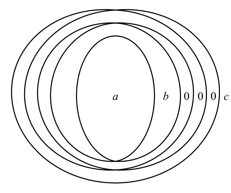 Figure 1
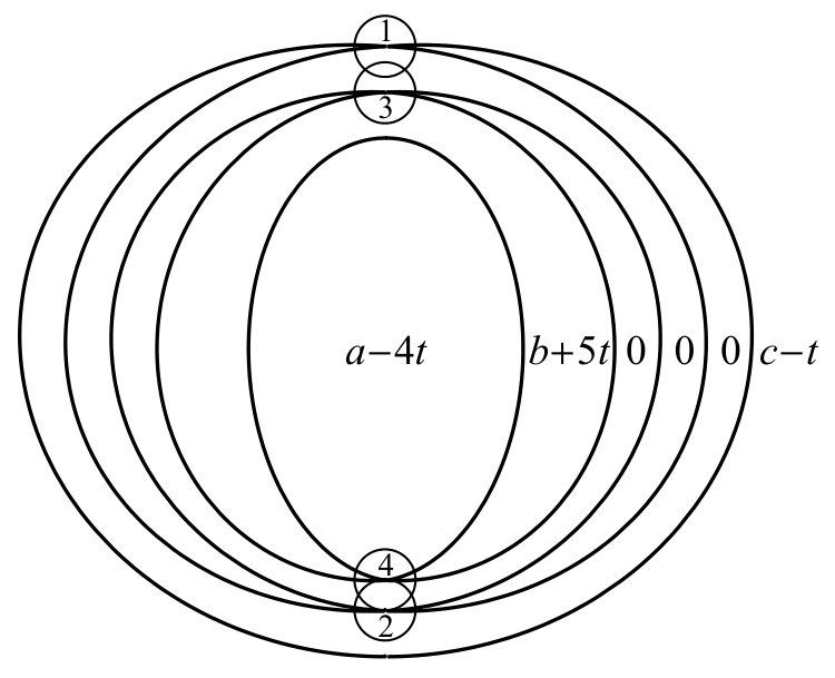 Figure 2
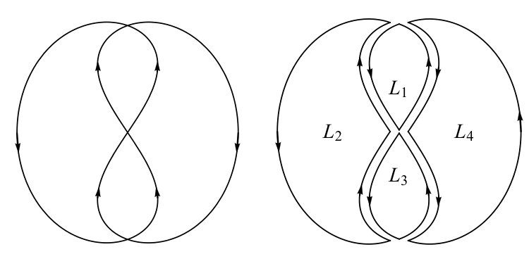 Figure 3
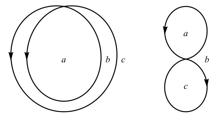 Figure 4
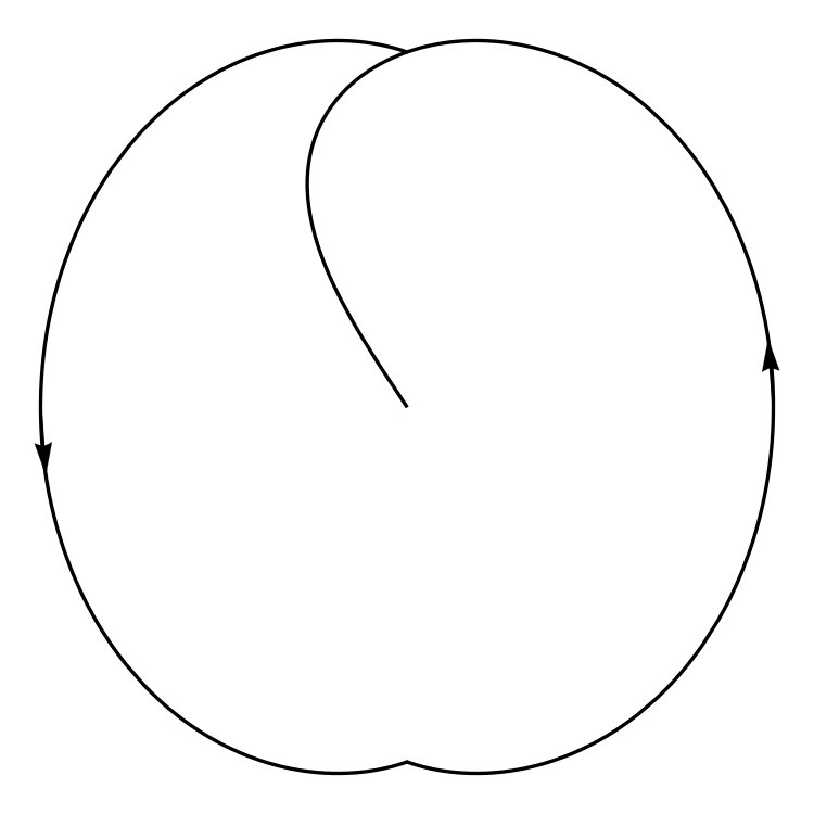 Figure 5
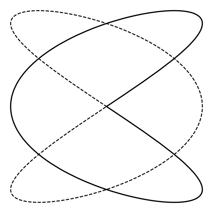 Figure 6
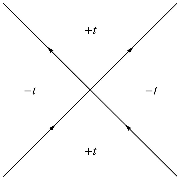 Figure 7
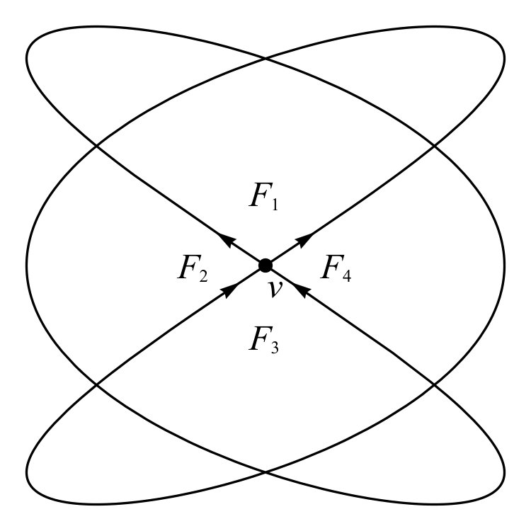 Figure 8
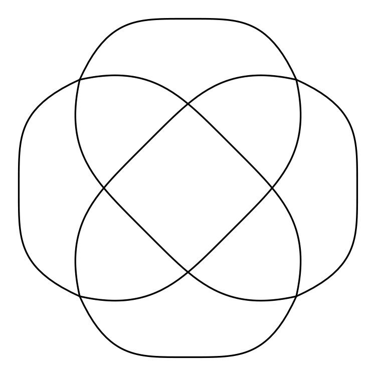 Figure 9
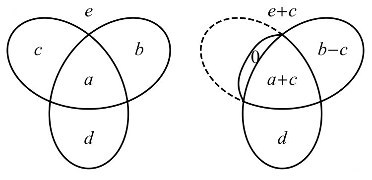 Figure 10
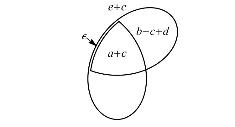 Figure 11
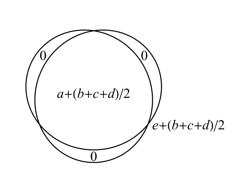 Figure 12
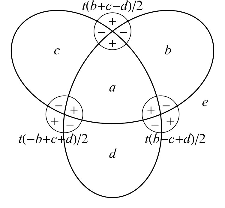 Figure 13
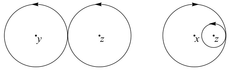 Figure 14
Peer Reviews
No public reviews on file for this paper yet. If you reviewed it on a platform where reviews are public (OpenReview, ICLR, NeurIPS, ICML), you can paste yours below so the community can read it here.
Videos
No videos yet. Explain this paper in a talk, walkthrough, or lecture? Add one.
The large- limit for two-dimensional Yang–Mills theory
Brian C. Hall
University of Notre Dame
Department of Mathematics
Notre Dame, IN 46556 USA
[email protected] Supported in part by NSF Grant DMS-1301534.
Abstract
The analysis of the large- limit of Yang–Mills theory on a surface proceeds in two stages: the analysis of the Wilson loop functional for a simple closed curve and the reduction of more general loops to a simple closed curve. In the case of the 2-sphere, the first stage has been treated rigorously in recent work of Dahlqvist and Norris, which shows that the large- limit of the Wilson loop functional for a simple closed curve in exists and that the associated variance goes to zero.
We give a rigorous treatment of the second stage of analysis in the case of the 2-sphere. Dahlqvist and Norris independently performed such an analysis, using a similar but not identical method. Specifically, we establish the existence of the limit and the vanishing of the variance for arbitrary loops with (a finite number of) simple crossings. The proof is based on the Makeenko–Migdal equation for the Yang–Mills measure on surfaces, as established rigorously by Driver, Gabriel, Hall, and Kemp, together with an explicit procedure for reducing a general loop in to a simple closed curve. The methods used here also give a new proof of these results in the plane case, as a variant of the methods used by Lévy.
We also consider loops on an arbitrary surface . We put forth two natural conjectures about the behavior of Wilson loop functionals for topologically trivial simple closed curves in Under the weaker of the conjectures, we establish the existence of the limit and the vanishing of the variance for topologically trivial loops with simple crossings that satisfy a “smallness” assumption. Under the stronger of the conjectures, we establish the same result without the smallness assumption.
Contents
1 Introduction and main results
1.1 The Makeenko–Migdal equation in two dimensions
Let us fix a connected compact Lie group together with an Ad-invariant inner product on its Lie algebra, The path integral for Euclidean Yang–Mills theory over a manifold is supposed to describe a probability measure on the space of connections for a principal -bundle over One of the main objects of study in such a theory is the Wilson loop functional, namely the expectation value of the trace (in some fixed representation of ) of the holonomy of the connection around a loop. The Makeenko–Migdal equation is an identity for the variation of Wilson loop functionals with respect to a variation in the loop. The original version of this equation, in any number of dimensions, was proposed by Makeenko and Migdal in [MM]. A version specific to the two-dimensional case was then developed by Kazakov and Kostov in [KK, Eq. (24)]. (See also [K, Eq. (9)] and [GG, Eq. (6.4)].)
A special feature of the two-dimensional Yang–Mills measure is its invariance under area-preserving diffeomorphisms. Suppose we fix the topological type of a loop in a surface and consider the faces of that is, the connected components of the complement of in Then the Wilson loop functional depends only on the areas of the faces of Let us now take with the inner product on the Lie algebra given by the scaled Hilbert–Schmidt inner product,
[TABLE]
It is then convenient to express the Wilson loop functionals in terms of the normalized trace,
[TABLE]
We now consider a loop with (a finite number of) simple crossings, and we let be one such crossing. We label the four faces of adjacent to the crossing in cyclic order as with denoting the face whose boundary contains the two outgoing edges of We then let denote the areas of these faces. (See Figure 1.) We also let denote the loop from the beginning to the first return to and let denote the loop from the first return to the end. (See Figure 2.)
The two-dimensional version of the Makeenko–Migdal equation, in the case, is then as follows:
[TABLE]
where denotes the holonomy. Although the curves and occurring on the right-hand side of (3) are simpler than the loop , the right-hand side of (3) involves the expectation of the product of the traces, rather than the product of the expectations. Thus, even if one has already computed the Wilson loop functionals and the right-hand side of (3) cannot be regarded as a known quantity. In the large- limit, however, we will see that the Makeenko–Migdal equation becomes an effective tool for inductive computation of Wilson loop functionals.
The original argument of Makeenko and Migdal for the equation that bears their names was based on heuristic manipulations of the path integral. In the plane case, Lévy then gave a rigorous proof of the Makeenko–Migdal equation in [Lév2]. (See Eq. (159) in Proposition 9.2.2 of [Lév2].) Subsequent proofs of the planar Makeenko–Migdal equation were then provided by Dahlqvist [Dahl] and Driver–Hall–Kemp [DHK2].
Meanwhile, in [DGHK], Driver, Gabriel, Hall, and Kemp gave a rigorous derivation of the Makeenko–Migdal equation for Yang–Mills theory over an arbitrary surface. Actually, the proof given in [DHK2] in the plane case extends with minor modifications to the case of a general surface.
1.2 The master field in two dimensions
In the paper [’t H], ’t Hooft proposed that Yang–Mills theory for in any dimension should simplify in the limit as In particular, it is expected that in this limit, the path integral should concentrate onto a single connection (modulo gauge transformations), known as the master field. The concentration phenomenon for the Yang–Mills measure has an important implication for the form of the two-dimensional Makeenko–Migdal equation. Specifically, in the limit, there should be no difference between the expectation of a product of traces and the product of the associated expectations: both and should become where is the master field.
If, therefore, the large- limit of Yang–Mills theory exists on a surface we expect it to satisfy a Makeenko–Migdal equation of the form
[TABLE]
where is the limiting value of Note that the loops and on the right-hand side of (4) have fewer crossings than since neither nor has a crossing at Thus, one may hope that the large- Makeenko–Migdal equation may allow one to reduce computations of Wilson loop functionals for general curves to simpler ones, until one eventually reaches a simple closed curve. Of course, since a simple closed curve has no crossings, the Makeenko–Migdal equation gives no information about the Wilson loop for such a curve.
In the plane case, the structure of the master field was worked out by Singer [Si], Gopakumar and Gross [GG, Gop], Xu [Xu], Sengupta [Sen4], Anshelevich and Sengupta [AS], and then in greater detail by Lévy [Lév2]. In particular, the expected concentration phenomenon was verified in detail in the plane case in [Lév2]. (See the explicit variance estimate in Theorem 6.3.1 of [Lév2].) A generalization of the master field on the plane was then constructed by Cébron, Dahlqvist, and Gabriel in [CDG].
In [Lév2], Lévy shows that the large- limit of the Wilson loop functional for a loop in the plane with simple crossings is completely determined by (4), together with another, simpler condition. This simpler condition—given as Axiom on p. 11 of [Lév2] and called the “unbounded face condition” in [DHK2, Theorem 2.3]—gives a simple formula for the derivative of the Wilson loop functional with respect to the area of any face of that adjoins the unbounded face.
1.3 The master field on the sphere
The existence of a large- limit of Yang–Mills theory on a general surface is currently unknown. There has, however, been much interest in the problem because of connections with string theory, as developed by Gross and Taylor [Gr, GT1, GT2].
The case, meanwhile, has been extensively studied at varying levels of rigor. The analysis proceeds in two stages. First, one studies the large- limit of the Wilson loop functional for a simple closed curve. Second, one attempts to use the large- Makeenko–Migdal equation to reduce Wilson loop functionals for all other loops with simple crossings to the simple closed curve.
In the first stage of analysis, a formula was proposed in the physics literature for the Wilson loop functional for a simple closed curve. (See Section 1.5 for more information.) A notable feature of this formula is the presence of a phase transition. If the total area of the sphere is less than the Wilson loop for a simple closed curve is expressible in terms of the semicircular distribution from random matrix theory. If, however, the total area is greater than the Wilson loop is much more complicated. In addition to the proposed formula for the limiting Wilson loop functional, it is expected that the limit should be deterministic, in keeping with the idea of the master field. This brings us to the following recent rigorous result of Dahlqvist and Norris [DN].
Theorem 1** (Dahlqvist–Norris)**
If is a simple closed curve on then the limit
[TABLE]
exists and depends continuously on the areas of the two faces of Furthermore, the associated variance tends to zero:
[TABLE]
The method of proof used in [DN] is discussed briefly in Section 1.5.
Notation 2
We denote the large- limit of the Wilson loop functional for a simple closed curve by :
[TABLE]
where is a simple closed curve and where and are the areas of the faces of
In the second stage of analysis, it has been claimed by Daul and Kazakov that, “All averages for self-intersecting loops can be reproduced from the average for a simple (non-self-intersecting) loop by means of loop equations.” (See the abstract of [DaK]. The loop equations referred to are the large- Makeenko–Migdal equation (4).) It should be noted, however, that Daul and Kazakov analyze only two examples, and it is not obvious how to extend their analysis to general loops; see Section 3. Furthermore, they assume that the large- limit exists and satisfies the large- Makeenko–Migdal equation.
1.4 The reduction procedure
In this paper, we give a rigorous treatment of the second stage of the analysis of the large- limit for Yang–Mills theory on as well as results for the plane and general surfaces. (Dahlqvist and Norris also give treat the case by a similar but not identical method, as discussed further in Section 1.4.1.)
1.4.1 On the sphere
Specifically, we establish the following results in the sphere case: (1) the existence of the large- limit of Wilson loop functionals for arbitrary loops with simple crossings; (2) the vanishing of the associated variance; and (3) the large- Makeenko–Migdal equation for the limiting theory. In particular, we give a concrete procedure for reducing the Wilson loop functional for general loops in to the Wilson loop functional for a simple closed curve.
Here are some notable features of our approach.
- •
We do not assume the existence of the large- limit ahead of time, except for a simple closed curve (Theorem 1).
- •
We do not assume ahead of time that the limiting theory satisfies the large- Makeenko–Migdal equation. Rather, we assume only the finite- Makeenko–Migdal equation in (3), as established rigorously in [DGHK]. We then prove that the limiting theory satisfies a large- version of the equation.
- •
We give a constructive procedure for reducing the Wilson loop functional an arbitrary loop in with simple crossings inductively to that for a simple closed curve. Specifically, we show that any loop can first be reduced to one that winds times around a simple closed curve, which can then be reduced to a simple closed curve.
The just-referred-to procedure relies on a result (Proposition 10) that says that it is possible to perform a combination of Makeenko–Migdal variations at all of the vertices, with the effect that the areas of all but two of the faces shrink to zero, with the areas of the remaining two faces remaining non-negative. Furthermore, it is possible to choose one of the “unshrunk” faces arbitrarily.
After the first version of this paper was posted to the arXiv, I became aware of a preprint of Dahlqvist and Norris [DN], which had been posted approximately two months earlier. The paper of Dahlqvist and Norris proves Theorem 1, which I stated as a conjecture in the first version of this paper. In addition, [DN] gives a reduction procedure that is similar to, but not identical to, the one I use here. The main difference between the two approaches is the just-mentioned freedom in my approach to arbitrarily choose one of the faces whose area does not shrink to zero. This flexibility is exploited crucially to give results on arbitrary surfaces, as discussed in Sections 1.4.2 and 6.
Our main result on the sphere may be stated as follows.
Theorem 3
If is a closed curve traced out on a graph in and having only simple crossings, the following results hold. First, the limit
[TABLE]
exists and depends continuously on the areas of the faces of Second, the associated variance goes to zero:
[TABLE]
Third, the limiting expectation values satisfy the following large- Makeenko–Migdal equation. Let us vary the areas of the faces surrounding a crossing in a checkerboard pattern as in Figure 3, resulting in a family of curves Then
[TABLE]
where and are derived from in the usual way.
In Figure 3, we do not assume the four faces are distinct. If, say, the two faces labeled as are the same, we are then increasing the area of that face by
The reason for stating the Makeenko–Migdal equation in the form in (9) is that we have not established the differentiability of the large- Wilson loop functional with respect to the area of an individual face. If this differentiability property turns out to hold, we can then apply the chain rule to express the derivative on the left-hand side of (9) in the usual form as an alternating sum of such derivatives. This issue is of little consequence, since the result in (9) is the way one applies the Makeenko–Migdal equation in all applications.
1.4.2 On the plane and on arbitrary surfaces
We also provide a new proof of Theorem 3 in the plane case, as a variant of the methods used by Lévy in [Lév2]. In the plane case, the result is not dependent on results of [DN], since the analog of Theorem 1 for is a simple computation; see Section 5.1. In Lévy’s analysis in [Lév2], the structure of the master field on is based on two main axioms, the large- version of the Makeenko–Migdal equation and a second condition, labeled as Axiom in [Lév2, Section 0] and called the “unbounded face condition” in [DHK2, Theorem 2.3], which gives a formula for the derivative of a Wilson loop functional with respect to the area of any face that adjoins the unbounded face. (There are also some continuity and invariance properties.) We show that the master field on can alternatively be characterized by the large- Makeenko–Migdal equation together with the (simple) formula for the Wilson loop for a simple closed curve. See Section 5.
Finally, we consider Yang–Mills theory on an arbitrary compact surface Let us call a loop in “topologically trivial” if it is contained in a topological disk We put forth two natural conjectures regarding topologically trivial simple closed curves in . The first, Conjecture 16, is simply the obvious analog of Theorem 1 for topologically trivial simple closed curves. (No such result is known for surfaces other than the plane and the sphere.) The second, Conjecture 19, asserts also similar results for a loop that winds times around a simple closed curve, Assuming the first conjecture, we establish the analog of Theorem 3 for topologically trivial loops with simple crossings that satisfy a “smallness” assumption. Assuming the second conjecture, we establish the analog of Theorem 3 for all topologically trivial loops with simple crossings. See Section 6.
Our results for the plane and for arbitrary surfaces depend crucially on an extra level of flexibility in the reduction process that is not present in [DN]. This paper and [DN] both use an approach in which the areas of all but two of the faces of the curve are shrunk to zero. In the procedure in [DN, Section 4.5], one generically has no choice regarding which two faces remain unshrunk; they are specified by conditions on the winding numbers. In our approach, by contrast, one of the unshrunk faces can be chosen arbitrarily. In the plane case, we choose one of the unshrunk faces to be the unbounded face, while in the case of an arbitrary surface, we choose one of the unshrunk faces to be the one containing the complement of the topological disk
1.5 The Wilson loop for simple closed curve in
In this section, we describe three approaches (at varying levels of rigor) to analyzing the Wilson loop functional for a simple closed curve in the sphere. If is a simple closed curve on and the areas of the two faces of are and Sengupta’s formula [Sen1] reads
[TABLE]
where is a normalization factor. Here is the heat kernel on based at the identity and evaluated at “time” The probability measure
[TABLE]
is precisely the distribution at time of a Brownian bridge on starting at the origin and returning to the origin at time
In the first approach, one writes the heat kernels in (10) as sums over the characters of the irreducible representations of In the large- limit, one attempts to find the “most probable representation,” that is, the one whose character contributes the most to the sum. The representations, meanwhile, are labeled by certain diagrams; the objective is then to determine the limiting shape of the diagram for the most probable representation. Using this method, physicists have found different shapes in the small-area phase (namely ) and the large-area phase (namely ). (See works by Douglas and Kazakov [DoK] and Boulatov [Bou].)
At a rigorous level, Boutet de Monvel and Shcherbina [BS] and Lévy and Maïda [LM] have analyzed the partition function (i.e., the normalization factor ) by this method and confirmed the existence of a phase transition at Then, recently, Dahlqvist and Norris [DN, Section 3] have given a rigorous analysis of the Wilson loop functional using a rigorous version of the arguments in [DoK] and [Bou], leading to Theorem 1.
In the second approach, one writes the heat kernels in (10) as a sum over all geodesics connecting the identity to using a formula developed by Èskin [Ès] and rediscovered by Urakawa [Ur]. (This formula is a Poisson-summed version of the formula as a sum of characters.) When the quantities and in (10) are small, the contribution of the shortest geodesic dominates. Recall that we are using the scaled Hilbert–Schmidt inner product (1) on the Lie algebra Since the Laplacian scales oppositely to the inner product, the Laplacian on is scaled by a factor of compared to the Laplacian for the unscaled Hilbert–Schmidt inner product. Thus, at a heuristic level, the large- limit ought to be pushing us toward the small-time regime for the heat kernels and It is therefore possible that in the large- limit, one can simply “neglect the winding terms,” that is, include only the contribution from the shortest geodesic.
The contribution of the shortest geodesic, meanwhile, is a Gaussian integral of the sort that arises in the Gaussian unitary ensemble (GUE) in random matrix theory. Thus, if it is valid to keep only the contribution from the shortest geodesic, the Wilson loop functional may be computed using results from GUE theory. (See the work of Daul and Kazakov in [DaK].) On the other hand, a consistency argument indicates that neglecting the winding terms can only be valid in the small area phase. Little work has been done, however, in estimating the size of the winding terms.
In the third approach, one may, as we have noted, recognize the probability measure in (11) as the distribution of a Brownian bridge on Forrester, Majumdar, and Schehr have then developed a method [FMS] to represent the partition function for Yang–Mills theory in terms of a collection of nonintersecting Brownian bridges on the unit circle. (That is, we consider Brownian motions in the unit circle, starting at 1. We then constrain them to return to 1 at time and to be nonintersecting for all times ) In fact, the distribution of the eigenvalues of the Brownian bridge in is precisely the distribution of these nonintersecting Brownian bridges. This claim is presumably well known to experts—I learned it from Thierry Lévy—and is explained in the notes [Ha2]. (The claim is analogous to the well-known result that the eigenvalues of a Brownian motion in the space of Hermitian matrices are described by the “Dyson Brownian motion” [Dys] in See Section 3.1 of [Tao].) Thus, not just the partition function, but also the Wilson loop functional for a simple closed curve can be expressed in terms of nonintersecting Brownian bridges.
Meanwhile, Liechty and Wang [LW1, LW2] have obtained various rigorous results about the large- behavior of the nonintersecting Brownian bridges in . In particular, they confirm the existence of a phase transition: When the lifetime of the bridge is less than the nonintersecting Brownian motions do not wind around the circle, whereas for lifetime greater than they do. It is possible that one could establish Theorem 1 rigorously in the small-area phase using results from [LW1]. (Theorem 1.2 of [LW1] would be relevant.) In the large-area phase, however, [LW1] does not provide information about the distribution of eigenvalues when is close to half the lifetime of the bridge. (See the restrictions on in Theorem 1.5(a) of [LW1].)
2 Tools for the proof
In this section, we review some prior results that will allow us to prove our main theorem. Our main tool, besides the crucial result of Dahlqvist and Norris in Theorem 1, is the Makeenko–Migdal equation for Yang–Mills theory on compact surfaces, which was established at a rigorous level in [DGHK]. More precisely, we require not only the standard Makeenko–Migdal equation in (3), but also an “abstract” Makeenko–Migdal equation, which allows us to compute the alternating sum of derivatives of expectation values of more general functions. We also require an estimate on the variance of the product of two bounded random variables, as described in Section 2.2.
2.1 Variation of the Wilson loop and of the
variance
Rigorous constructions of the two-dimensional Yang–Mills measure with structure group from a continuum perspective were given in the plane case by Gross, King, and Sengupta [GKS] and by Driver [Dr], and in the case of a compact surface, possibly with boundary, by Sengupta [Sen1, Sen2, Sen3]. (See also [Lév1], which, among other things, extends the analysis to rectifiable loops with infinitely many self-intersections.) In particular, suppose is an “admissible” graph in a surface meaning that contains the boundary of and that each face of is a topological disk. Let denote the number of unoriented edges of and let be a gauge-invariant function of the connection that depends only on the parallel transports along the edges of Then Driver (in the plane case) and Sengupta (in the general case) give a formula for the expectation value of with respect to the Yang–Mills measure. The formulas of Driver and Sengupta correspond to what is known as the heat kernel action in the physics literature, as developed by Menotti and Onofri [MO] and others.
Let denote the heat kernel on based at the identity. Then we have, explicitly,
[TABLE]
where denotes the normalized Haar measure on , is the area of the th face, and is the product of edge variables going around the boundary of Here is a normalization constant. Since is invariant under conjugation and inversion, the formula does not depend on the starting point or orientation of the boundary of If the boundary of is nonempty, it is possible to incorporate into (12) constraints on the holonomies around the boundary components; the proof of the Makeenko–Migdal equation in [DGHK] holds in this more general context.
Remark 4
In the rest of the paper, when we speak about “varying the areas” of the faces of graph, we mean more precisely that we replace the numbers by some other collection of positive real numbers in Sengupta’s formula (12). If the sum of the ’s equals the sum of the ’s, it may be possible to implement this variation “geometrically,” by continuously deforming the graph, but this is not necessary. In particular, the Makeenko–Migdal equation (3) was proved under such an “analytic” (i.e., not necessarily geometric) variation of the area.
If we have a fixed loop and we let the areas of the faces of depend on a parameter we will (in a small abuse of notation) denote that pair consisting of and the collection of areas by
Suppose now that is a loop that can be traced out on an oriented graph in and let be a minimal graph on which can be traced. We now explain what it means for to have a simple crossing at a vertex . First, we assume that has exactly four edges incident to , where we count an edge twice if both the initial and final vertices of are equal to . Second, we assume that , when viewed as a map of the circle into the plane, passes through exactly twice. Third, we assume that each time passes through , it comes in along one edge and passes “straight across” to the cyclically opposite edge. Last, we assume that traverses two of the edges on one pass through and the remaining two edges on the other pass through .
Under these assumptions, Theorem 1 of [DGHK] gives a rigorous derivation of the Makeenko–Migdal equation in (3). We now restate the Makeenko–Migdal equation for in the case, in a way that facilitates the large- limit. In addition, we derive a similar result for the variation of the variance of where for a complex-valued random variable , we define
[TABLE]
Proposition 5
Let be a loop traced out on a graph in and having only simple crossings. Let be one such crossing and let and be obtained from as usual in the Makeenko–Migdal equation. Then we have
[TABLE]
and
[TABLE]
where and are the composite curves and Here denotes the covariance, defined as
Proof. Equation (13) is simply the Makeenko–Migdal equation (3) rewritten using the definition of the covariance. To establish (14) we need to use the abstract Makeenko–Migdal equation established in Theorem 2 of [DGHK]. (This result generalizes the abstract Makeenko–Migdal equation formulated and proved for the plane case by Lévy in [Lév2, Proposition 9.1.3].) Following the argument in Section 2.3 of [DHK2], we express the loop as
[TABLE]
where and are words in edges other than Then and If are the edge variables corresponding to we then have (following the convention that parallel transport is order reversing)
[TABLE]
where and are words in the edge variables other than
Now, the abstract Makeenko–Migdal equation reads
[TABLE]
whenever has “extended gauge invariance” at the vertex When the edges are distinct, extended gauge invariance at means that
[TABLE]
for all where is the collection of edge variables other than (See Section 4 of [DHK2] for a discussion of extended gauge invariance when the edges are not distinct.)
Let us apply (15) to the function where
[TABLE]
We also use the notation
[TABLE]
We then note that
[TABLE]
Now, as verified in [DHK2, Eqs. (2.13)–(2.15)], we have . Meanwhile, using for and computing as in the second example in [DHK2, Section 2.5], we have that
[TABLE]
Thus,
[TABLE]
Meanwhile, by the ordinary Makeenko–Migdal equation (3), we have
[TABLE]
Subtracting (17) from (16) gives the claimed result.
2.2 Variance estimates
For a complex-valued random variable we define the variance of by
[TABLE]
In particular,
[TABLE]
We then define the standard deviation of denoted , by
We observe that for any two random variables and we have
[TABLE]
and similarly for any number of random variables. (It is harmless to assume that the expectation values of and —and therefore —are zero, in which case (19) is the triangle inequality for the norm.) We also consider the covariance of two random variables, defined as
[TABLE]
(For our purposes, it is convenient not to put a complex conjugate into this definition; the reader should note that .) We record the elementary inequality
[TABLE]
which follows from (20) and the Cauchy–Schwarz inequality.
We now establish a simple estimate on the standard deviation of the product of two bounded random variables.
Proposition 6
Suppose and are two complex-valued random variables satisfying and . Then
[TABLE]
Proof. For simplicity of notation, let and let Thus, Then since we have and Then by (18) and the Cauchy–Schwarz inequality, we have
[TABLE]
since and similarly for Now,
[TABLE]
because adding a constant does not change the variance. Thus, by (19),
[TABLE]
which reduces to the claimed formula.
3 Examples
Before developing a general method for analyzing a general loop in with simple crossings, we consider two illustrative examples, the same two that are considered in [DaK].
3.1 The figure eight
Although we consider loops on we can draw them as a loops on the plane by picking a face and placing a puncture in that face, so that what is left of is identifiable with We need to keep in mind, however, that the “unbounded” face in such a drawing is actually a bounded face (with finite area) on Furthermore, by placing the puncture in different faces, the same loop on can give inequivalent loops on As a simple example, consider the loop in Figure 4, which we refer to as the figure eight. Figure 4 gives two different views of this loop coming from puncturing two different faces.
We write the holonomy around the figure eight as
[TABLE]
to indicate the dependence of the Wilson loop functional on the areas. In this case, the loops and occurring on the right-hand side of the Makeenko–Migdal equation are both simple closed curves. The loop (the outer loop on the left-hand side of Figure 4, which is the lower loop on the right-hand side of the figure) encloses areas and . The loop (the inner loop on the left-hand side of the figure, which is the upper loop on the right-hand side of the figure) encloses areas and .
Theorem 7
The limit
[TABLE]
exists and satisfies the large- Makeenko–Migdal equation in the form
[TABLE]
where is as in Notation 2. Furthermore, we have
[TABLE]
See (26) for a formula for in terms of the function . If the partial derivatives of with respect and exist and are continuous, it follows from the chain rule that
[TABLE]
The following proof, however, does not establish the existence or continuity of the partial derivatives of
Proof. We denote the holonomies for the two loops and as and . The face labeled as should be the one bounded by the two outgoing edges of at which is the face with area Then coincides with while and are the faces with areas and (in either order). We assume with the case being entirely similar.
Proposition 5 takes the form
[TABLE]
Let us denote by (with , and fixed). We then write ; that is,
[TABLE]
Now, it should be clear geometrically that if we let the area in the figure eight tend to zero, the result is a simple closed curve. That is to say, we expect that
[TABLE]
where is a simple closed curve on enclosing areas and Analytically, (25) follows easily from Sengupta’s formula, using that converges to a -measure on as tends to zero. Thus, letting tend to zero, we obtain
[TABLE]
Note that all holonomies on the right-hand side of (26) are of simple closed curves. If we use (6) in Theorem 1 together with the inequality (22) and dominated convergence, we find that the last term in (26) tends to zero as tends to infinity. Then using (5) in Theorem 1 along with dominated convergence, we may let to obtain
[TABLE]
for where is as in Notation 2. (Note that the normalized trace defined in (2) satisfies for all so that dominated convergence applies in both integrals in (26).) This result establishes the first claim in the theorem.
If we now subtract the value of (27) at and the value at we obtain
[TABLE]
Dividing this relation by and letting tend to zero gives
[TABLE]
by the continuity of This relation is the desired large- Makeenko–Migdal equation.
Meanwhile, by the second relation in Proposition 5, we have
[TABLE]
The first term on the right-hand side tends to zero as tends to infinity, by Theorem 1. In the second term on the right-hand side, and are simple closed curves. Furthermore, the normalized trace satisfies for all Thus, using (22) and Proposition 6 together with Theorem 1, we see that the second term on the right-hand side of (28) tends to zero. Finally, since the last term on the right-hand side manifestly goes to zero.
3.2 The trefoil
In this section, we briefly outline an analysis of the trefoil loop by a method similar to the one in the previous subsection. Later we will develop a systematic method for analyzing any loop; this will provide an alternative analysis of the trefoil. We label the areas of the faces as in Figure 5, where we may assume without loss of generality that We now perform a Makeenko–Migdal variation at the vertex in the top middle of the figure. In this case, the loops and turn out to be simple closed curves.
Let us denote by the loop on the right-hand side of Figure 5. Then is the limit as tends to zero of the loops in Figure 6, where denotes the distance between the two nearby arcs of the loop. Specifically, in Figure 6, we let tend to zero, while keeping all of the areas of the faces fixed to the values indicated, using the continuity properties of the Wilson loop functional developed in [Lév1, Theorem 2.58]. But, is independent of and we conclude that But since the loop is of the type analyzed in Section 3, we may already know the large- behavior of The argument then proceeds much as in Section 3.1; since we will develop later a systematic method for analyzing arbitrary loops, we omit the details of this analysis.
Other examples are not quite so easy to simplify by using the Makeenko–Migdal equation at a single vertex. In the loop in Figure 7, for example, it is not evident how shrinking any one of the faces to zero simplifies the problem.
4 Analysis of a general loop
4.1 The strategy
Given an arbitrary loop traced out on a graph in with simple crossings, we will consider a linear combination of Makeenko–Migdal variations of the areas over all the vertices of We will show that it is possible to make such a variation, depending on a parameter in such a way that as tends to 1, all but two of the areas of the faces tend to zero. Thus, in the limit, we effectively have a loop with only two faces. Indeed, we will show that the limit of the Wilson loop functional is the Wilson loop functional for a loop that winds times around a simple closed curve. Here is an integer determined by the topology of the original loop (A similar but not identical procedure is used in [DN]. See Section 4.4 for a comparison.)
Consider, for example, the trefoil loop of Section 3.2. If we vary the areas by the amounts shown in Figure 8, the net effect on the areas is:
[TABLE]
Thus, as varies from [math] to the areas and shrink simultaneously to zero, while the areas of the two remaining faces increase. The limiting curve is shown in Figure 9. If the areas of the three lobes are zero, the curve becomes a circle traversed twice.
Let denote the trefoil with areas varying as above. If we differentiate with respect to then by the chain rule, we will get a linear combination of terms of the form
[TABLE]
where and represent the loop cut at the th vertex of the trefoil (), along with some covariance terms. Each and is actually a simple closed curve, but in any case, these curves have fewer crossings than the original trefoil. It is then a straightforward matter to let tend to infinity to get the limiting Wilson loop functional, and similarly for the variance.
For an arbitrary loop with crossings, we will show that we can deform into a loop that winds times around a simple closed curve. The variation of the Wilson loop functional along this path will be a linear combination of products of Wilson loop functionals for curves with at most crossings. In an inductive argument then, it remains only to analyze which we do by another induction, this time reducing to and so on.
4.2 Winding numbers
We consider with a fixed orientation. We then consider a loop traced out on a graph in and having only simple crossings. We consider the faces of that is, the connected components of the complement of in If we pick a face we can puncture , thus turning topologically into The orientation on gives an orientation on Thus, for each face we may speak about the winding number of around Since this winding number depends on which face we puncture, we denote it thus:
[TABLE]
so that It is important to understand how the winding number changes if the location of the puncture changes.
Proposition 8
If and are faces, then
[TABLE]
In particular, the difference between and does not depend on
In particular, if we change the location of the puncture, all the winding numbers change by the same amount.
Proof. Let us fix points and in and respectively. Let us put our puncture initially in regarding as the plane. Let us then assume that is at the origin and is at the point . We may then regard as an element of with base point at which is a free group on two generators and . These generators may be identified with circles of radius one centered at and respectively, traversed in the counter-clockwise direction. Then is the number of times winds around which is the number of occurrences of the generator in the representation of as a word in and
Suppose we now shift our puncture from to This shift amounts to composing with the inversion map in the complex plane, that is, the map After this process, the generator traverses the unit circle in the opposite direction, while the generator is now inside the unit circle (Figure 10). Thus, is the number of occurrences of minus the number of occurrences of giving the claimed result.
4.3 The span of the Makeenko–Migdal vectors
Let be a loop traced out on a graph in and having only simple crossings. We consider vectors assigning real numbers to the faces of For each vertex of we define the Makeenko–Migdal vector associated to denoted as
[TABLE]
where are the four faces surrounding If, for example, are distinct, then is the vector that assigns the numbers to respectively, and zero to all other faces.
Theorem 9** (T. Lévy)**
Fix a face of and let be a vector assigning a real number to each face of Then belongs to the span of the Makeenko–Migdal vectors if and only if (1) is orthogonal to the constant vector and (2) is orthogonal to the winding-number vector
This result is the case of Lemma 9.4.3 in [Lév2]. Note that by Proposition 8, the winding number vector associated to some other face differs from by a multiple of the constant vector . Thus, if is orthogonal to then is orthogonal to if and only if is orthogonal to Thus, the condition in the theorem is independent of the choice of
4.4 Shrinking all but two of the faces
Let denote the number of faces of We now choose one face arbitrarily and denote it by . We will show that there is another face such that we can perform a Makeenko–Migdal variation of the areas in which the areas of the faces shrink simultaneously to zero, while the area of increases or remains the same. In the generic case, the area of also remains positive, while in a certain borderline case, the area of tends to zero as well.
The freedom we have to choose one of the “unshrunk” faces arbitrarily will be essential in applications to the plane and to arbitrary surfaces. This freedom is a difference between our approach and the one used in [DN], where the two unshrunk faces in Section 4.5 are chosen to have maximal and minimal winding numbers.
Proposition 10
Assume has at least three faces. Choose one face arbitrarily and let all winding numbers be computed relative to a puncture in , so that Let denote the vector of areas of the faces and let be the vector of winding numbers. Suppose and adjust the labeling of so that is maximal among the winding numbers if and is minimal if . Then there exists in the span of the Makeenko–Migdal vectors such that (1) all the entries of are non-negative for and (2) has the form with and .
Meanwhile, if , there exists in the span of the Makeenko–Migdal vectors such that (1) all the entries of are non-negative for and (2) has the form with .
The proposition says, briefly, that we can shrink to zero without decreasing and while keeping non-negative.
In the case of the trefoil loop, for example, suppose we take to be the “unbounded” face in Figure 8 and we orient the loop in the counter-clockwise direction. Then the winding numbers are 1 for the three lobes of the trefoil and 2 for the central region. Since all winding numbers are positive in this case, we always have in which case we take to the central region. Figures 8 and 9 then illustrate Proposition 10.
Proof. Assume first that , in which case, the maximal winding number must be positive. In light of Theorem 9, two vectors and differ by a vector in the span of the Makeenko–Migdal vectors if and have the same inner products with the constant vector and the winding number vector . To achieve these conditions, we first set equal to and equal to 0. Since , we then have , regardless of the value of . Next, we choose to achieve the condition . Now, . Then since is maximal, we have
[TABLE]
Thus, , which shows that . (In particular, .) Since both and have non-negative entries, so does every point along the line segment joining them. The analysis of the case is similar.
Finally, if , we may set and all other entries of equal to zero. In that case, and , showing that differs from by a vector in the span of the Makeenko–Migdal vectors.
4.5 Analyzing the limiting case
As a consequence of Proposition 10, we may start with an arbitrary loop and perform a linear combination of Makeenko–Migdal variations at each vertex, obtaining a family of loops with the same topological type with all but two of the areas shrinking to zero as We now analyze the behavior of the Wilson loop functional in the limit
We will analyze the limit “analytically,” using Sengupta’s formula for the finite- case. (Recall Remark 4.) For this result, the structure group can be an arbitrary connected compact Lie group
Theorem 11
Let be a loop traced out on a graph in and having only simple crossings. Denote the number of faces of by and label the faces as Suppose we vary the areas of the faces as a function of a parameter in such a way that as the areas of tend to zero, while the areas of and approach positive real numbers and , respectively. Then
[TABLE]
where is the winding number of around relative to a puncture in and is a normalization constant. Meanwhile, if the area of also tends to zero in the limit, then
[TABLE]
The integral on the right-hand side of (29) is just the Wilson loop functional for a loop that winds times around a simple closed curve enclosing areas and Note that the winding number of around is the same as the winding number of the original loop around Note also that by Theorem 9, the value of for the loop is independent of for Since and through are tending to zero, this means that must be tending to the value where is the winding number of around It then follows that the limiting loop has the same value of even though has a different topological type from .
Proof. Let be a minimal oriented graph on which can be traced. We think of as a graph in the plane, by placing a puncture into If denotes the number of edges of then we may consider two different measures on : the Yang–Mills measure for viewed as a graph in the plane and the Yang–Mills measure for viewed as a graph in the sphere. By comparing Sengupta’s formula [Sen1, Sect. 5] in the sphere case to Driver’s formula [Dr, Theorem 6.4] in the plane case, we see that
[TABLE]
where is the collection of edge variables, is the area of as a face in and is the product of edge variables around the boundary of Here is a normalization constant.
We may rewrite both of the Yang–Mills measures using “loop variables” as follows. Let us fix a vertex and a spanning tree for Then in Section 5.3 of [Lév2], Lévy gives a procedure associating to the faces certain loops in that constitute free generators for , based at (Note that there is no generator associated to the face ) Each is a word in the edges of We may then associate to each of the faces of a loop variable, which is the product of edge variables in (in the reverse order, since parallel transport reverses order). The map sending the collection of edge variables to the collection of loop variables defines a map where is the number of edges of
According to Proposition 5.3.3 of [Lév2], the loop variables are independent heat-kernel distributed random variables with respect to (See also Proposition 12.7 of [Ga].) That is to say, the push-forward of under is just the product of heat kernels, at times equal to the areas of the faces. Although there is no generator associated to the face the generate Suppose, therefore, that is a loop that starts at travels along a path to a vertex in then around the boundary of and then back to along Then is expressible as a word in and therefore is expressible as a word in the loop variables: for some function on (Although depends on the choice of and the invariance of the heat kernel under conjugation guarantees that is well defined.) It then follows from the measure-theoretic change of variables theorem that the push-forward of is given by
[TABLE]
Meanwhile, the loop (whose Wilson loop functional we are considering) is also expressible as a word in the generators (See Figure 11.) Thus,
[TABLE]
It is now straightforward to take a limit in (30) as that is, as all areas other than and tend to zero. In this limit, each heat kernel associated to becomes a -measure, so we simply evaluate each such to the identity element of giving
[TABLE]
In the sphere case, the normalization factor is given by where is the total area of the sphere. Although may depend on (since we do not currently assume that the area of the sphere is fixed), it has a limit as
If the limiting value of is also zero, then becomes also becomes a -function. Since the normalized trace of the identity matrix equals 1, the right-hand side of (31) becomes But the total area of the sphere in this limit is just so and
Finally, if the limiting value of is nonzero, we must understand the effect on and of evaluating to the identity. Recall that the words and arise from representing the boundary of and the loop as words in which are free generators for . Now, is naturally isomorphic to where is an arbitrarily chosen element of There is then a homomorphism from to induced by the inclusion of into Since is just a free group on the single generator this homomorphism is computed by mapping each of the generators to the identity, leaving only powers of Thus, if we write, say, as a word in the generators and apply the just-mentioned homomorphism, the result will be where is the winding number of around (i.e., around ). By the Jordan curve theorem, this winding number is assuming that we traverse in the counter-clockwise direction. (In Figure 12, for example, the outer boundary of the loop in Figure 11 decomposes as ; if we set any three of the four generators to the identity, the remaining generator will occur to the power 1.) Expressing this result in terms of the loop variables, rather than the loops themselves, we conclude that is . Similarly, where is the winding number of around
4.6 The induction
In this section, we prove Theorem 3 by induction on the number of crossings. Our strategy is to deform an arbitrary loop with crossings into a loop that winds times around a simple closed curve. The variation of the Wilson loop functional along this deformation will be a linear combination of products of Wilson loop functionals for curves with fewer crossings, plus a covariance term. We begin by recording a result for a loop that winds times around a simple closed curve.
Theorem 12
Let denote a loop that winds times around a simple closed curve enclosing areas and Then for all and the limit
[TABLE]
exists and depends continuously on and Furthermore, the associated variance tends to zero:
[TABLE]
The proof of this result is given in Section 4.7. Assuming Theorem 12 for the moment, we are now ready for the proof of our main result.
Proof of Theorem 3. Let denote the number of crossings of We will proceed by induction on When the result is precisely Theorem 1. Assume, then, that (7) and (8) and the continuity condition hold for all loops with crossings and consider a loop with crossings. Using Proposition 10, we may make a combination of Makeenko–Migdal variations at the vertices of giving loops in which and so that all but two of the faces shrink to zero as By Theorem 11, the limit as of the Wilson loop functional of is the Wilson loop functional of a loop that winds times around a simple closed curve enclosing areas and where and are the areas of the two remaining faces. We may differentiate the Wilson loop functional of using the chain rule and the first part of Proposition 5. Integrating the derivative then gives
[TABLE]
where the constants are the ones expressing the vector in Proposition 10 as a linear combination of the Makeenko–Migdal vectors Here and are the loops obtained by applying the Makeenko–Migdal equation at the vertex to the loop In particular, since neither of these loops has a crossing at we see that and have at most crossings.
By our induction hypothesis, the limit
[TABLE]
exists for each each and each Our induction hypothesis also tells us that the variance of goes to zero as ; the inequality (22) then tells us that the covariances on the last line of (32) also tend to zero. Now, for all from which it follows that . Thus, we may apply dominated convergence to all integrals in (32), along with Theorem 12, to obtain
[TABLE]
establishing the existence of the limit in (7) of Theorem 3.
We now establish the claimed continuity of with respect to the areas of the faces. For each topological type of loop we fix an arbitrary face to play the role of in the proof of Proposition 10. We then fix two other faces with maximal and minimal winding numbers, respectively, relative to a puncture in . The first key observation is that with these choices made, the vector in the proof of the proposition can be chosen to depend continuously on the areas of the faces. If we compute by the formula in the proof, the only case in which continuity is not obvious is in the case in which (in the notation of the proof) But a moment’s thought will confirm that as tends to zero, tends to the vector where is the area of which is just the value of when
Now, when we deform our original loop into a loop of the form the values of and depend continuously on the areas of the faces of ; indeed, and are the first two entries of the vector The continuity of also gives the continuity of and thus of the coefficients in (33), which are the coefficients of the expansion of in terms of the Makeenko–Migdal vectors. Thus, the continuity of the second term on the right-hand side of (33) follows from our induction hypothesis and dominated convergence.
To establish the second claim (8) of Theorem 3, we use the second part of Proposition 5. We then need to bound the covariance term appearing in (14). We first use (22) and then use Proposition 6 to bound the variance of the product of and The argument is then similar to the proof of (7).
Finally, we establish the large- Makeenko–Migdal equation (9) for the limiting Wilson loop functionals. If we vary the areas in a checkerboard pattern along a path as in Figure 3, we have
[TABLE]
Using the first two points (7) and (8) in Theorem 3, we can let tend to infinity to obtain
[TABLE]
Since we have shown that depends continuously on the areas of we see that and depend continuously on Thus, we can apply the fundamental theorem of calculus to differentiate (34) with respect to to obtain the large- Makeenko–Migdal equation (9).
4.7 The -fold circle
In this section, we analyze the Wilson loop functional for a loop that winds times around a simple closed curve, establishing Theorem 12. Similar results were obtained by Dahlqvist and Norris in [DN, Section 4.5].
Recall from (11) that the distribution of the parallel transport around a simple closed curve is the distribution of a Brownian bridge in Assuming that the eigenvalue distribution of a Brownian bridge in has a deterministic large- limit, the calculations here provide a recursive method for computing the higher moments of the limiting distribution, in terms of the first moment. (But the formula for the first moment is complicated, especially in the large-lifetime phase, ) A similar, but not identical, recursion for the moments of the free unitary Brownian motion—i.e., the large- limit of a Brownian motion in rather than a Brownian bridge—was established by Biane. See the bottom of p. 16 of [Bi1] and p. 266 of [Bi2].
We approximate a loop that winds times around a simple closed curve by a loop with simple crossings, specifically, by a curve of the “loop within a loop within a loop” form, as in Figure 13. If there are a total of loops, then there are crossings and a total of faces. The faces divide into the innermost circle, the outer region, and annular regions. Shifting the puncture from the innermost to outermost regions gives another curve of the same sort, with the order of the annular regions reversed.
Now, nothing prevents us from letting the areas of one or more of the annular regions equal zero. Specifically, we may understand the limit as some of the areas tend to zero by the same method as in the proof of Theorem 11. The only difference is that in the expression (30), we set an arbitrary subset of the loop variables equal to the identity. We may similarly make a Makeenko–Migdal variation at one or more of the vertices and then take a limit on both sides of the resulting equation as some of the areas tend to zero.
If we set the areas of the annular regions to zero, the curve will simply wind times around the outermost circle. More generally, we will show that it is possible to shrink the central region and the outer region, while increasing the innermost annular region and keeping the areas of the outermost annular regions equal to zero, as in Figure 13. This observation motivates consideration of the following class of loops.
Definition 13
Let denote the loop that winds times around a simple closed curve enclosing areas and Now let be a simple closed curve having two faces and with areas and respectively. For let denote the loop that winds times around and then winds once around a region of area inside
When we interpret as being (the loop that winds zero times around around and then once around a region of area ).
We may consider two different limiting cases of the case where tends to zero and the case where tends to zero. If tends to zero, we are left with while if tends to zero, we are left with (To see this, it may be useful to shift the puncture from the face to the face, as on the right-hand side of Figure 4.) We now give an inductive procedure for computing the limiting Wilson loop functionals for loops of the form and
Theorem 14
For all and all non-negative real numbers and the limits
[TABLE]
and
[TABLE]
exist, and the associated variances tend to zero. Furthermore, for all we have the following inductive formulas. If we have
[TABLE]
If, on the other hand, we have
[TABLE]
Our main interest is in the quantity which is the same as Note, however, that even if we put on the left-hand side of (37) or (38), the right-hand side of the equation will still involve with nonzero values of On the other hand, the inductive procedure ultimately expresses —and thus, in particular, —in terms of
Suppose, for example, that we wish to compute in terms of Since is symmetric in and it is harmless to assume that so that (37) applies. We first compute in terms of , by applying (37) with (since ) giving
[TABLE]
(This formula is just what we obtained in (27) in Section 3.1.) We then apply (37) with and giving
[TABLE]
Last, we plug into (40) the values of and computed in (39).
In the case of the assumption that guarantees that so that we may directly apply (39). In the case of , there may be some values of for which we need to use the symmetry of with respect to and before applying (39). If, however, we may directly apply (39) to the computation of for all
Some explicit computations of these expressions in the plane case (i.e., the case) are given in Section 5.2.
Proof of Theorem 14. The argument is similar to the proof of Theorem 3, except with a different variation of the areas. We assume, inductively, that the limits in (35) and (36) exist for all . We also assume that the corresponding variances go to zero. (When this claim is just Theorem 1.) We then prove these results for while also proving the inductive formulas (37) and (38).
We consider the loop We realize this loop by starting with an -fold “loop within a loop within a loop,” with the areas of the outermost annular regions set equal to , and then letting tend to zero. We then order the crossings from outermost to innermost. We then make a Makeenko–Migdal variation at the th crossing, scaled by a factor of (See Figure 14.) The resulting change in the areas is
[TABLE]
while the areas of the outer annular regions remain unchanged.
If the area of the outermost region will remain non-negative as the area of the innermost region shrinks to zero. Thus, we may apply the Makeenko–Migdal equation (13) with the annular areas equal to and then let tend to zero, giving a finite- version of (37):
[TABLE]
Here and and “” is a covariance term.
Then, as in the proof of the first two points of Theorem 3, our induction hypothesis, together with (22) and Proposition 6, allows us to take the limit with the covariance term going to zero. Thus, the large- limit of exists for and satisfies (37). The vanishing of the variance then follows by the same argument as in the proof of Theorem 3.
An entirely similar argument applies when using a finite- version of (38), establishing existence of the limit and vanishing of the variance for for all non-negative values of and The limit in (35) and vanishing of the variance then follow by setting
5 The plane case, revisited
5.1 The general result
In [Lév2], Thierry Lévy establishes the large- limit of Wilson loop functionals for Yang–Mills theory in the plane, together with the vanishing of the associated variances. (See Theorem 9.3.1 in [Lév2].) The limiting expectation values for loops with simple crossings are then characterized in [Lév2] by the large- Makeenko–Migdal equation and another condition, labeled as Axiom in Section 0 of [Lév2] and termed the unbounded face condition in Theorem 2.3 of [DHK2].
The methods of the present paper give a new proof of some of these results, making it possible to treat the cases of the plane and the sphere in a uniform way. Specifically, the proof of Theorem 3 applies with minor changes in the plane case. Furthermore, the analog of Theorem 1 is easily established by direct computation in the plane case, as we will demonstrate shortly. We thus obtain a characterization of the master field on the plane slightly different from the one in [Lév2]; both characterizations use the large- Makeenko–Migdal equation, but ours replaces the unbounded face condition with the (simple!) formula for the Wilson loop functional of a simple closed curve in the plane.
Theorem 15
Theorem 3 holds also in the plane case.
Proof. We follow the same argument as in the case of the sphere, with a few minor modifications. First, in Section 4.4, we should choose to the unbounded face, so that the areas are finite numbers. Theorem 11 still holds, with the same proof, in the plane case, provided we interpret as being the constant function (The normalization factor is then also equal to 1.) All other proofs go through without change—except that in Section 4.7, the condition always holds because .
We now supply the proof of the plane case of Theorem 1. Of course, the claim follows from results in [Lév2] (see Theorem 6.3.1), but we can give a elementary proof as follows.
Proof of Theorem 1 for . The function is an eigenfunction for the Laplacian on —with respect to the scaled Hilbert–Schmidt metric in (1)—with eigenvalue (See, e.g., Remark 3.4 in [DHK1].) It follows that for a simple closed curve enclosing area we have
[TABLE]
It is also possible to compute the (complex) variance of explicitly. Using results from Section 3 of [DHK1], we may easily compute that
[TABLE]
(We have used that ) Thus, the space of functions spanned by and 1 is invariant under and the action of on this space is represented by the matrix
[TABLE]
We may exponentiate times this matrix using elementary formulas for the exponential of matrices (e.g., Exercise 5 or Exercises 6 and 7 in [Ha1, Chapter 2]), with the result that
[TABLE]
so that
[TABLE]
Thus, the complex variance of is
[TABLE]
which goes to zero as tends to infinity.
More generally, Theorem 1.20 in [DHK1] identifies the leading-order term in the large- asymptotics of the Laplacian, acting on “trace polynomials” (that is, sums of products of traces of powers of ). This leading term satisfies a first-order product rule. Thus, the limiting heat operator is multiplicative, from which it follows that the variance of any trace polynomial vanishes as (See the last displayed formula on p. 2620 of [DHK1].)
5.2 Example computations in the plane case
We now illustrate the computation of large- Wilson loop functionals in the plane case. We first compute the large- Wilson loop functionals from Section 4.7 in the plane case, which corresponds to for The condition is always satisfied in that case, and, as noted in the previous subsection, the Wilson loop functional for a simple closed curve is
The two-fold circle. When (37) takes the following form:
[TABLE]
which agrees with Lévy’s formula for the “loop within a loop” in the appendix of [Lév2]. When we get which is the second moment of Biane’s distribution for the free unitary Brownian motion. (The moments may be found in Lemma 3 of [Bi1] or the Remark on p. 267 of [Bi2].)
The three-fold circle. When and (40) becomes
[TABLE]
All the -terms in the exponents cancel, leaving us with times polynomials. Direct computation of the integral then gives
[TABLE]
which agrees with the case of the last of Lévy’s examples of loops with two crossings in the appendix of [Lév2]. When we get which is the third moment of Biane’s distribution.
The trefoil. We now analyze the large- Wilson loop functional for the trefoil loop in the plane case, using the strategy outlined in Section 4.1. In this example, the loops and occurring on the right-hand side of the Makeenko–Migdal equation are simple closed curves for all , and the product of the Wilson loop functionals simplifies as
[TABLE]
where the dependence on and drops out. Thus, when we integrate from to , we obtain simply the constant value of the integrand. Now, the signs in the Makeenko–Migdal variations in Figure 8 are reversed from usual labeling. After adjusting for this and noting that the coefficients of the variations in Figure 8 add to , we obtain
[TABLE]
Using the value for computed above and simplifying gives
[TABLE]
which agrees with the value of the master field for the trefoil in the appendix of [Lév2].
6 General compact surfaces
6.1 Introduction
We now consider the Yang–Mills measure on a compact surface possibly with boundary. (See [Sen3] and also [Lév1].) If the boundary of is nonempty, we may optionally impose constraints on the holonomy around the boundary components. The Makeenko–Migdal equation in this setting was established rigorously in [DGHK].
Let us say that a loop in is topologically trivial if it is contained in an (open) topological disk All results in this section pertain only to topologically trivial loops. For a topologically trivial simple closed curve in one may reasonably expect that the analog of Theorem 1 will hold, but the author is not aware of any results in this direction.
Suppose, however, that we simply assume that the analog of Theorem 1 holds for topologically trivial simple closed curves in We will then establish the analog of Theorem 3—not for all topologically trivial loops, but only for those satisfying a “smallness” condition. The reason for the smallness assumption is as follows. Suppose is a loop in a topological disk and let denote the face of that contains the complement of in Then in the first stage of deformation, following the procedure in Section 4.4, we perform a Makeenko–Migdal variation of to a loop that winds times around a simple closed curve. This first variation can be done in such a way that the area of does not decrease, so that the deformed loop can be chosen to remain in . In the second stage of deformation, we try to reduce—as in Section 4.7—from a curve that winds times around a simple closed curve to a curve that winds only once around a simple closed curve. In this second variation, the area of will unavoidably decrease and may become zero, unless the original loop is “small.” If the area of becomes zero, the deformation process becomes undefined, because the limit of the Wilson loop as tends to zero is not easily evaluated (except when is a topological disk, i.e., when is a sphere).
On the other hand, suppose we assume that a natural strengthening of Theorem 1 holds for topologically trivial loops in . Specifically, suppose we simply assume that Theorem 1 holds not only for topologically trivial simple closed curves in , but also for curves that wind times around a topologically trivial simple closed curve. Then the second stage of deformation in the previous paragraph is not needed. Under this assumption, therefore, we will be able to prove Theorem 3 for all topologically trivial loops in
Let us consider what the previous discussion means for the study of the master field on a general compact surface The analysis will have two stages, as in the case: A direct calculation for the case of simple closed curves, and a reduction of general curves to the simple closed case using the Makeenko–Migdal equation. If we hope to use the just-discussed results for general surface, more must be put into the direct calculation stage.
For a simple closed curve in Sengupta’s formula gives a probability measure on which describes the distribution of the holonomy of a random connection around If we ultimately wish to analyze all topologically trivial loops with simple crossing, then in the direct calculation stage of analysis, we will have to look not just at the first moment of
[TABLE]
but also at the higher moments,
[TABLE]
which are just the Wilson loop functionals for curves that wind times around If one could establish directly (i.e., without using the Makeenko–Migdal equation) the existence of the large- limit and the vanishing of the variance for the quantities in (42) and (43), then the results of this section would apply to give the existence of the limit and vanishing of the variance for all topologically trivial loops with simple crossings.
6.2 Statements
We begin by stating the analog of Theorem 1 for topologically trivial loops in as a conjecture.
Conjecture 16
Consider a surface of area Let be a topological disk and consider a simple closed curve in . In Sengupta’s formula for the Yang–Mills measure on , let us assign area to the interior of and area
[TABLE]
to the exterior of for any Then the limit
[TABLE]
exists and depends continuously on and and
[TABLE]
We now introduce a notion of “smallness” for a general loop in with simple crossings. We may cut a loop in at a crossing, obtaining two loops and . We may then cut either or at one of its crossings, and so on. We refer to any loop that can be obtained by a finite sequence of such cuts as a subloop of In particular, is a subloop of itself corresponding to making zero cuts. We label the faces of as where is the face containing the complement of
For a loop in and a point that is in but not in we define the winding number of around by considering the homotopy class of in with respect to a fixed orientation on Next, we define, for each face of
[TABLE]
where the maximum ranges over all subloops of and all and where is the winding number of around Finally, if is the area of we define
[TABLE]
Remark 17
One may bound as follows. Suppose for some one can travel from any face of to while crossing at most times. Then the same is true of any subloop of Since the winding number of is zero and changes by one each time we cross we conclude that is at most
Theorem 18
Assume Conjecture 16. Let be a loop traced out on a graph in a topological disk with simple crossings. Then Theorem 3 holds for , provided satisfies the “smallness” assumption
[TABLE]
where and are defined in (44) and (45), respectively.
Note that since is contained in a disk, is certainly homotopically trivial in Thus, Theorem 18 does not tell us anything about homotopically nontrivial loops. Since is a topological disk, Theorem 9 applies in this context, provided we compute the winding numbers of the faces of by regarding as a loop in
We next state a natural extension of Conjecture 16.
Conjecture 19
Continuing with the notation of Conjecture 16, let denote the loop obtained by traveling times around Then for all the limit
[TABLE]
exists and depends continuously on and and
[TABLE]
Assuming Conjecture 19 holds, we can prove Theorem 3 for topologically trivial loops in without imposing a smallness assumption.
Theorem 20
Assume Conjecture 19. Let be a loop with only simple crossing, traced out on a graph in a topological disk in . Then Theorem 3 holds for without any smallness assumption on
6.3 Proofs
Let be a topological disk in and let be a loop traced out on a graph in and having only simple crossings. We follow the deformation process in Section 4.4, with the face whose area does not decrease taken to be the face of containing The obvious analog of Theorem 11 continues to hold (see Lemma 22 below), so that at the end of the deformation process, we obtain a loop that winds times around a simple closed curve in We may apply the same deformation process to all the subloops generated by the Makeenko–Migdal equation, and again the area of will not decrease. Thus, if we assume the stronger assertion in Conjecture 19, we may prove Theorem 20 precisely as in Section 4.6, but using Conjecture 19 in place of Theorem 12.
If, on the other hand, we wish to assume only the weaker assertion in Conjecture 16, we must proceed to the second stage of analysis, deforming the loop that winds times around a simple closed curve to one that winds once around a simple closed curve, as in Section 4.7. In this stage of analysis, the area of will unavoidably decrease, unless . If the area of becomes zero during the deformation, the whole process fails, because there is no easy way to compute the limit of a Wilson loop functional as the area of goes to zero. (See (50), in which the limit as goes to zero is not easily computed. The only case where this limit is easy to evaluate is when is a topological disk, that is, when is a sphere.)
In the case of a curve winding times around a simple closed curve, there is a simple condition (Theorem 21) on the and the enclosed area guaranteeing that the area of will remain positive. We must then show that the smallness condition in Theorem 18 guarantees that each “-fold circle” generated by will satisfy the hypotheses of Theorem 21.
Theorem 21
Let the notation be as in Conjecture 16. For each nonzero integer let denote the loop that winds times around Assuming Conjecture 16, Theorem 3 holds for provided that
[TABLE]
Proof. It is harmless to assume Following the proof of Theorem 12 in the sphere case, we deform into a loop of the form Let denote the vector of areas of the faces of and let be the associated vector of winding numbers, viewing as a loop in the disk with We will actually prove Theorem 21 for the loops by induction on under the assumption that
[TABLE]
which reduces to (47) when and When , the loop is (by definition) the same as so that the desired result is just Conjecture 16. For we may follow the same sort of inductive argument as in the sphere case, provided that we never shrink the area of the “” region to zero.
Take and assume that Theorem 21 holds for loops of the form satisfying (48), with Consider a loop satisfying (48) and deform it into the loop with as in Section 4.7. As we vary the values of and the values of and remains constant—as can be seen explicitly or as a consequence of Theorem 9. Thus, by (48), we have
[TABLE]
Since (49) tells us that
Thus, remains positive as approaches when we obtain a loop of the form with
[TABLE]
We can then see explicitly that the value of for is the same as for namely Thus, by induction, Theorem 18 holds for Furthermore, the loops and obtained from the Makeenko–Migdal equation will be or with It is then easy to see that the value of for these loops is no bigger than for which is the same as for Thus, and satisfy (48) and by induction, Theorem 18 holds for these loops as well.
From this point, the argument is the same as in the sphere case. In particular, since we have ensured that remains positive as we deform the areas of , we may apply (41) to compute the Wilson loop functional for
We now prove Theorem 18. Following the logic in Section 4, we first deform into a loop of the form Since the area of increases during this process, there is no obstruction to carrying out this first step in the analysis of Nevertheless, we require a smallness assumption on that will ensure that the limiting loop will satisfy the hypothesis of Theorem 21. This smallness assumption must also be inherited by the loops and occurring on the right-hand side of the Makeenko–Migdal equation, so that these loops can be analyzed by induction on the number of crossings.
Proof of Theorem 18. We proceed by induction on the number of crossings. If the result is Conjecture 16. Assume, then, that the result holds for loops with fewer than crossings and consider a loop with crossings. As in Lemma 22, we deform into a loop By the Makeenko–Migdal equation, the variation of the Wilson loop functional will involve loops of the form and all of which have fewer than crossings. We need to verify (1) that satisfies and (2) that and both satisfy the smallness assumption (46). If so, we may apply Theorem 21 to the loops and our induction hypothesis to and and the argument is then the same as in the sphere case.
For Point (1), we note that the value of is (Lemma 22) the winding number of around while the value of is the limiting value of (the area of ) as approaches 1. Now, on the one hand, the value of for is independent of by Theorem 9. On the other hand, approaches the value as approaches 1, since and for Thus, . But from the definitions (45) and (44) of and we have and thus
[TABLE]
For Point (2), we note that for the loops the area of is always increasing (Proposition 10), meaning that is decreasing. Thus, for all and we have
[TABLE]
Furthermore, since every subloop of is also a subloop of we see that Thus, we have
[TABLE]
Having verified these two points, the proof now proceeds as in the sphere case.
It remains only to verify that the analog of Theorem 11 holds for loops in
Lemma 22
Consider the Yang–Mills measure on for an arbitrary connected compact Lie group Let be a loop traced out on a graph in and having only simple crossings. Denote the number of faces of by and label the faces as where is the face containing Suppose we vary the areas of the faces as a function of a parameter in such a way that as the areas of tend to zero, while the areas of and approach non-negative real numbers and respectively, with Then
[TABLE]
where is the winding number of around .
Proof. Let be a minimal graph (necessarily connected) in which can be traced. Before we can apply Sengupta’s formula, we must embed into an admissible graph , that is, one that contains the boundary of and each of whose faces is a topological disk. Actually, by the Jordan curve theorem, all the faces of other than will automatically be disks. It is then possible to construct by adding new edges entirely in the closure of (See Section 1.2 of [Lév1].) Thus, the faces of may be chosen to be of the form where is a subset of having the same area as Let us divide the edge variables for into the edge variables corresponding to the original graph and the remaining edge variables Then integration with respect to the Yang–Mills measure for the graph in may be written as
[TABLE]
where and are the number of edges of and , respectively. Furthermore, we may write
[TABLE]
for some word in the variables. Here, for notational simplicity, we consider the unconditional Yang–Mills measure, but a similar argument applies if there are constraints on the holonomies around the boundary components of
In the case that is the trace of the holonomy of we may imitate the proof of Theorem 11 to obtain
[TABLE]
As in that proof, if we let we obtain
[TABLE]
where is the winding number of around But the right-hand side of (51) is just Sengupta’s formula for the Wilson loop functional for the loop that winds times around the boundary of (i.e., the outer boundary of ), enclosing areas and
7 Acknowledgments
The author thanks Bruce Driver, David Galvin, Todd Kemp, Thierry Lévy, Karl Liechty, Andy Putman, Ambar Sengupta, and Steve Zelditch for valuable discussions. The author is also grateful to Franck Gabriel for a detailed reading of the entire manuscript, along with many corrections and helpful suggestions. Finally, the author thanks the two referees, whose careful reading and thoughtful comments have improved the manuscript immensely.
The reference list from the paper itself. Each links out to its DOI / PubMed record.
- 1[AS] M. Anshelevich and A. N. Sengupta, Quantum free Yang-Mills on the plane. J. Geom. Phys. 62 (2012), 330–343.
- 2[Bi 1] P. Biane, Free Brownian motion, free stochastic calculus and random matrices. In : Free probability theory (Waterloo, ON, 1995), 1–19, Fields Inst. Commun. 12 , Amer. Math. Soc., Providence, RI, 1997.
- 3[Bi 2] P. Biane, Segal-Bargmann transform, functional calculus on matrix spaces and the theory of semi-circular and circular systems, J. Funct. Anal. 144 (1997), 232–286.
- 4[Bou] D. V. Boulatov, Wilson loop on a sphere, Mod. Phys. Lett. A 9 (1994), 365-374.
- 5[BS] A. Boutet de Monvel and M. Shcherbina, On free energy in two-dimensional U ( N ) 𝑈 𝑁 U(N) -gauge field theory on the sphere. (Russian) Teoret. Mat. Fiz. 115 (1998), 389–401; translation in Theoret. and Math. Phys. 115 (1998), 670–679.
- 6[CDG] G. Cébron, A. Dahlqvist, and F. Gabriel, The generalized master fields, J. Geom. Phys. 119 (2017), 34–53.
- 7[Dahl] A. Dahlqvist, Free energies and fluctuations for the unitary Brownian motion, Comm. Math. Phys. 348 (2016), 395–444.
- 8[DN] A. Dahlqvist and J. Norris, Yang-Mills measure and the master field on the sphere, preprint ar Xiv:1703.10578 [math.PR].