An improvement of the asymptotic Elias bound for non-binary codes
Krishna Kaipa

TL;DR
This paper develops a hybrid bound combining Elias and Plotkin bounds for non-binary codes, improving the upper bounds on the asymptotic information rate across different minimum distances.
Contribution
It introduces a new hybrid bound based on the anticode bound that outperforms existing bounds for non-binary codes.
Findings
The hybrid bound improves upon Elias and Plotkin bounds.
The anticode bound enhances the understanding of code rate limits.
Assuming a conjecture on convexity, the bounds follow directly.
Abstract
For non-binary codes the Elias bound is a good upper bound for the asymptotic information rate at low relative minimum distance, where as the Plotkin bound is better at high relative minimum distance. In this work, we obtain a hybrid of these bounds which improves both. This in turn is based on the anticode bound which is a hybrid of the Hamming and Singleton bounds and improves both bounds. The question of convexity of the asymptotic rate function is an important open question. We conjecture a much weaker form of the convexity, and we show that our bounds follow immediately if we assume the conjecture.
Click any figure to enlarge with its caption.
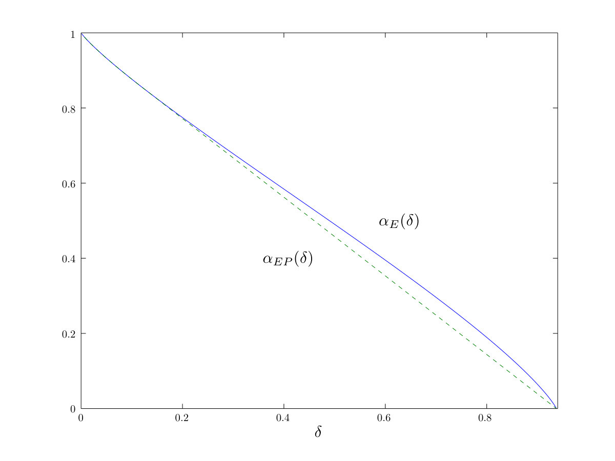 Figure 1
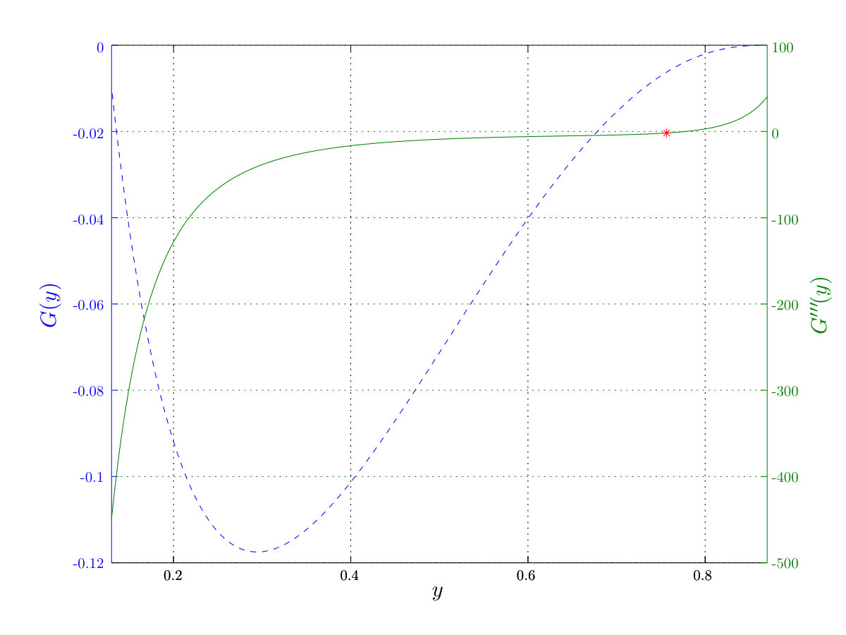 Figure 2
Peer Reviews
No public reviews on file for this paper yet. If you reviewed it on a platform where reviews are public (OpenReview, ICLR, NeurIPS, ICML), you can paste yours below so the community can read it here.
Videos
No videos yet. Explain this paper in a talk, walkthrough, or lecture? Add one.
An improvement of the asymptotic Elias bound for non-binary codes.
Krishna Kaipa K. Kaipa is with the Department of Mathematics at the Indian Institute of Science and Education Research, Pune 411008, India (email: [email protected]). The author was supported by the Science and Engineering Research Board, Govt. of India, under Project EMR/2016/005578.
Abstract
For non-binary codes the Elias bound is a good upper bound for the asymptotic information rate at low relative minimum distance, where as the Plotkin bound is better at high relative minimum distance. In this work, we obtain a hybrid of these bounds which improves both. This in turn is based on the anticode bound which is a hybrid of the Hamming and Singleton bounds and improves both bounds. The question of convexity of the asymptotic rate function is an important open question. We conjecture a much weaker form of the convexity, and we show that our bounds follow immediately if we assume the conjecture.
Index Terms:
information rate, size of a code, anticode.
I Introduction
Let denote the maximum size of a code of length , minimum distance at least , and contained in a subset , where is an alphabet of finite size . A central problem in coding theory is to obtain good upper and lower bounds for . The asymptotic version of this quantity is the asymptotic information rate function:
[TABLE]
The quantities and are related by the inequality
[TABLE]
known as the Bassalygo-Elias lemma. Taking to be a Hamming ball of diameter , and choosing optimally gives, at the asymptotic level the Hamming and the Elias upper bounds.
[TABLE]
[TABLE]
The bound is better than for all . Here is the entropy function (9), and .
An anticode of diameter in is any subset of with Hamming diameter . Let denote the maximum size of an anticode of diameter at most in . In contrast to the situation with , the quantity was explicitly determined by Ahlswede and Khachatrian in [1]. From their result, it is easy to determine the asymptotic quantity . We actually do not need the results of [1], however it is the main inspiration for this work. Taking to be an anticode in (2), and choosing optimally, we get the following two bounds which improve and respectively.
Theorem 1**.**
(hybrid Hamming-Singleton bound)
[TABLE]
The bound improves the Hamming and the Singleton bounds. It is -convex and continuously differentiable.
Theorem 2**.**
(hybrid Elias-Plotkin bound) Let .
[TABLE]
The bound improves the Elias and Plotkin bounds. It is -convex and continuously differentiable.
It is not known if the function itself is -convex, although it is tempting to believe that it is. We propose a weaker conjecture:
Conjecture 1**.**
The function is decreasing. In other words
[TABLE]
As evidence for this conjecture, we will show that theorems 1 and 2 follow very easily if we admit the truth of the conjecture.
The bound in Theorem 2 is an elementary and explicit correction to the classical Elias bound. It does not however improve the upper-bounds obtained by the linear programming approach, like the second MRRW bound (due to Aaltonen [2]) or the further improvement of due to Ben-Haim and Litsyn [3, Theorem 7]. The reasons for this are as follows: For small we have . For large , the inequality follows from the fact that has a non-zero slope at where as the actual function and the bound have zero slope at .
The paper is organized as follows. In section II, we collect some results on size of anticodes, which we use in section III to prove Theorems 1 and 2. We discuss Conjecture 1 in section IV.
II Size of anticodes
We recall that is the maximum size of an anticode of diameter at most in . If we take to be an anticode of size then clearly . Using this in (2), we get a bound
[TABLE]
known as Delsarte’s code-anticode bound [4]. Taking where we get
[TABLE]
Taking we get:
[TABLE]
where
[TABLE]
This is the the asymptotic form of (5). We use the notation and to denote a Hamming ball of radius in and its volume respectively. The ball where in is an anticode of diameter at most . Let and let be a fixed word. Sets of the form of size are also anticodes of diameter . It follows that:
[TABLE]
Here, we have used the well known formula:
[TABLE]
where,
[TABLE]
While the convexity of is an open question, it is quite easy to see that:
Lemma 1**.**
The function is -convex.
Proof:
If and are anticodes of diameters and respectively, then is an anticode of diameter . Taking to be anticodes, we immediately get
[TABLE]
Let go to infinity with , and . Applying to this inequality we get:
[TABLE]
∎
We note that with codes we have , which is why the above proof method does not apply to the question of convexity of . From (8) and Lemma 1 we get:
[TABLE]
Let . We can rewrite this as
[TABLE]
where is defined by
[TABLE]
We note that
[TABLE]
There is a unique positive number satisfying (where the Hamming and Singleton bounds intersect). Therefore, has the same sign as . Using this in (10), we see that for . Therefore, in order to maximize it suffices to consider . We note that has the same sign as and hence that of . Since , we see that for fixed , the function is maximized for . We are now reduced to maximizing
[TABLE]
Lemma 2**.**
Let for .
[TABLE]
Proof:
We calculate:
[TABLE]
Therefore . Next, we note that
[TABLE]
has the same sign as , as was to be shown. A stronger assertion is that is in fact -convex: differentiating once more, we get:
[TABLE]
We note that , and hence the first term is non-negative. The remaining parenthetical term is non-negative using the inequality
[TABLE]
and the fact that for . ∎
It follows from Lemma 2 that
[TABLE]
Therefore we obtain the bound:
Theorem 3**.**
* where*
[TABLE]
Moreover, is continuously differentiable and -convex.
We have used the relation
[TABLE]
The function is continuously differentiable because the component for is just the tangent line at to the component for , i.e. to . We note that equals for and for . Since is non-increasing, it follows that is -convex.
In the next lemma, we show that there is a sequence of anticodes of diameter at most such that equals , i.e. the lower bound on given in theorem 3.
Lemma 3**.**
Consider the anticodes of diameter in (taken from [1]) given by
[TABLE]
[TABLE]
Then .
Proof:
We note that
[TABLE]
Also equals
[TABLE]
which simplifies to if and (on using (14)) to if . This is the same as . ∎
We now have all the results we need for proving theorems 1 and 2. However, we will state a remarkable theorem due to Ahlswede and Khachatrian [1], which we will not need. We also obtain an asymptotic version of their result and record it as a corollary, as it does not seem to have appeared in literature. In brief their theorem states that equals . Moreover any anticode is Hamming isometric to the anticode (with some exceptions). At the asymptotic level, the result is again remarkable: The lower bound for given in theorem 3 is actually the exact value of . Moreover need not have been defined using as already exists.
Theorem**.**
[1]** Given and integers , let and be as in Lemma 3. Then,
[TABLE]
Moreover, up to a Hamming isometry of an anticode of size must be:
- •
**
- •
or with replaced with . This case is possible only if is a positive integer not exceeding .
Corollary 1**.**
[TABLE]
Proof:
It follows from the theorem of Ahlswede and Khachatrian, together with Lemma 3 that
[TABLE]
Therefore
[TABLE]
∎
III Proofs of theorems 1 and 2
III-A Proof of Theorem 1
If we use the bound of Theorem 3 in the inequality (see (6)), we obtain the bound
[TABLE]
Since is -convex and continuously differentiable (see Theorem 3), it follows that is -convex and continuously-differentiable. To show that , we note that being the secant line to between and , lies above the graph of as the latter is -convex. To prove that improves we note that coincides with for , and for , Lemma 2 implies that . This finishes the proof of Theorem 1.
It is worth noting that (12) implies the following formula for :
[TABLE]
Since for and , we get
[TABLE]
It can be shown (see subsection III-C) that is an upper bound for which improves both the Hamming and Plotkin bounds.
III-B Proof of Theorem 2
It will be convenient to identify the alphabet with the abelian group . Given , let and . We take to be the anticode (from Lemma 3):
[TABLE]
[TABLE]
We will take the balls to be centered at . As in Lemma 3, we have
[TABLE]
We also note that Lemma 3 gives
[TABLE]
Let be the maximum possible size of a code contained in and having minimum distance at least .
Theorem 4**.**
* if*
[TABLE]
Proof:
Our proof is similar to the standard proof of the analogous result for the Elias bound (which corresponds to taking instead of the prescription (18)). First let be a code of size , where is the anticode for some . Let
[TABLE]
where . We note that , and that
[TABLE]
We can rewrite this as:
[TABLE]
For we use Cauchy-Schwarz inequality to get . In particular
[TABLE]
Let be the projection of on to the factor . We note that for , we have wt because . Here wt is the number of nonzero entries of . Therefore
[TABLE]
Since we get:
[TABLE]
In particular
[TABLE]
We note that . By Cauchy-Schwarz inequality:
[TABLE]
[TABLE]
Since equals
[TABLE]
we get:
[TABLE]
This can be rewritten as:
[TABLE]
Combining this with (22) we get:
[TABLE]
Using (23) this can be written as:
[TABLE]
Now let be a sequence of codes of size . The preceding inequality gives:
[TABLE]
Using this in (21), we get:
[TABLE]
provided the denominator is a positive number. Therefore, provided
[TABLE]
This condition is the same as
[TABLE]
Since this finishes the proof. ∎
Using (2) we get:
[TABLE]
Taking as and using the result of Theorem 4 and (19) we get:
[TABLE]
where is the largest value of for which the inequality (20) holds. In order to determine , we introduce functions on defined by:
[TABLE]
Lemma 4**.**
Let .
* with equality only at .* 2. 2.
* is the tangent line to at .* 3. 3.
.
Proof:
Let . We observe that
[TABLE]
The three assertions to be proved follow respectively from the following three relations:
[TABLE]
∎
Proposition 1**.**
[TABLE]
The function is increasing, continuously differentiable, and -convex on .
Proof:
The inequality (20) reduces to
[TABLE]
where is as given in (18). Therefore, for a given , the quantity is the maximum element of the set
[TABLE]
If , then (by Lemma 4) and hence, the maximum of this set is . If , then (by Lemma 4) and hence, the maximum of this set is . This proves the asserted formula for .
We note that the second component of is the tangent line to the first component at . Therefore is continuously differentiable. The derivative of is for , and constant at for . Since the derivative is positive, the function is increasing. Since the derivative is non-decreasing, we see that the function is -convex. ∎
Proof of being an upper bound: We note from lemma 4 that
[TABLE]
Therefore is just the function defined in of theorem 2. The bound now follows from (24).
Proof of being continuously differentiable: The function being a composition of continuously differentiable functions, is itself continuously differentiable.
Proof of being -convex: Both the functions and are -convex, but is decreasing and hence it is not obvious that is -convex. We will show instead that the derivative is non-decreasing. Since is constant for , it suffices to show that for . This follows from the next lemma.
Lemma 5**.**
The Elias bound is -convex on and -convex on where satisfies:
[TABLE]
Proof:
Let . A calculation shows that
[TABLE]
[TABLE]
To see this, we note: and hence
[TABLE]
Since and , we get
[TABLE]
as desired. It follows that sign. Next we note that is increasing on and
[TABLE]
It now suffices to show that
[TABLE]
We note that
[TABLE]
Thus is decreasing on and increasing on . In order to show sign for some , it suffices to show that and . We calculate
[TABLE]
Since , we have . The inequality (11) implies that the first parenthetical term above is non-negative. Again implies
[TABLE]
and hence the second parenthetical term is positive. Thus .
Next, we note that . The function satisfies
[TABLE]
and . Therefore for , and hence for all .
∎
Proof that improves the Plotkin bound: We have already shown that is -convex, and hence lies below the secant line between and , which is the Plotkin bound.
Proof that improves the Elias bound: This does not readily follow from our results thus far, and requires more work. The characterization of given in the next theorem clearly implies .
Theorem 5**.**
**
Proof:
The theorem immediately follows if we show that is decreasing on and increasing on . We will use the notation from the proof of Lemma 5. Since is -convex for , it follows that the slope of the secant between and is increasing. It remains to show that is decreasing on and increasing on . Since is an increasing function, with , and , it suffices to show that
[TABLE]
is decreasing on and increasing on where . A calculation shows that
[TABLE]
To see this we note that either side of this equation evaluates to . Since for , we see
[TABLE]
Thus we have also shown that is decreasing for and increasing on as required. ∎
The bounds , and are related as
[TABLE]
We have already shown in (16). Since for all , we note that
[TABLE]
Thus . We end this section with a plot comparing and for .
III-C Another proof of Theorem 1
Another proof of being an upper bound for can be given using the following theorem of Laihonen and Litsyn:
Theorem**.**
[5]** Let .
[TABLE]
Proof:
We give a quick proof. The result follows from the inequality:
[TABLE]
by taking , and and going to and respectively. The above inequality in turn comes from the Bassalygo-Elias lemma (2)
[TABLE]
by taking , and observing that . (If is a code, and is the projection on the second factor, then the restriction of to is injective, and has minimum distance at least .)
∎
If we set , and in (27), we get:
[TABLE]
Thus,
[TABLE]
where we have used (15).
We now prove that the function defined in (16) is an upper bound for . Taking , , and in (27), we get:
[TABLE]
Thus
[TABLE]
It is not known if the inequality (27) (the theorem of Laihonen-Litsyn) holds if we replace by . If such a result were true, then the derivation of the bound above with replaced with would immediately yield Theorem 5. We believe that such an inequality
[TABLE]
must be true (it would surely be true if is -convex), but we believe it cannot be obtained just by a simple application of the Bassalygo-Elias lemma (2). If (29) holds, we can obtain an upper bound which improves the Laihonen-Litsyn bound [5]. We recall that the Laihonen-Litsyn bound, which we denote is a hybrid of the Hamming and MRRW bounds. It coincides with the Hamming bound for and with the MRRW bound for where are points such that the straight line joining and is a common tangent to both at and at . Since the Hamming bound is good for small and the MRRW bound good for large , the Laihonen-Litsyn bound combines the best features of both bounds in to a single bound. To obtain this bound, we note that (27) implies the inequality
[TABLE]
We fix and choose and optimally in order to minimize the right hand side. This yields the bound. Since the second MRRW bound improves the first MRRW bound , a better version of the Laihonen-Litsyn bound (see [3, Theorem 2]) can be obtained by using in place of . Since the Elias bound is better than the Hamming bound for all , in case (29) is true, repeating this procedure with replacing , would yield the hybrid Elias-MRRW bounds which would improve the respective Laihonen-Litsyn bounds . We leave the question of the truth of (29) open.
IV On the convexity of
A fundamental open question about the function is whether it is -convex. In other words is it true that
[TABLE]
It is worth noting that non-convex upper bounds like the Elias bound and the MRRW bound admit corrections to the non-convex part: the bound for the Elias bound and the Aaltonen straight-line bound (see the theorem below and the Appendix) for the MRRW bound. This may be viewed as some kind of evidence supporting the truth of (30). It is known that (30) holds for (for example by taking in (27)). Another way to state this is that
[TABLE]
As a consequence, if is any upper bound for we obtain a better upper bound
[TABLE]
To see this we use:
[TABLE]
Thus as desired. If is a decreasing function then the improved bound coincides with , but otherwise improves . For example let be the first MRRW bound
[TABLE]
It can be shown that that fails to be decreasing near , and similarly fails to be -convex near . This is immediately rectified by passing to the improved bound , resulting in the following theorem of Aaltonen.
Theorem**.**
(Aaltonen bound) [6] [7, p.53] Let . where
[TABLE]
This bound is -convex, continuously differentiable, and improves the MRRW bound.
We note that for the bound coincides with the tangent line to at . In particular is continuously differentiable. The assertion that improves follows from the fact that for any upper bound for . The other assertions are proved in the appendix.
On the other hand, it is not known if the convexity condition (30) holds for , in other words if is a decreasing function of . We conjecture that this is true (see Conjecture 1). As evidence for this conjecture, we now show that the bounds , and can be obtained without doing any work, if we assume the truth of Conjecture 1: if is any upper bound for we obtain a better upper bound
[TABLE]
To see this we use:
[TABLE]
Thus as desired. In case is a decreasing function then the improved bound coincides with , but otherwise improves . Taking to be the Elias bound, we get to be the bound . This is the content of Theorem 5. Taking to be the Hamming bound, we get to be the bound . This is the content of (28). Moreover, if is decreasing then being the product of the non-negative decreasing functions and is itself decreasing. Thus we obtain . Taking to be the Hamming bound, the bound is . This is the content of (15).
Appendix A Aaltonen’s straight-line bound
The bound presented above was obtained by Aaltonen in [6, p.156]. The bound follows from (31) and the following result
[TABLE]
The argmax above is not straightforward to obtain, and to quote from [6], was found by a mere chance. The derivation is not presented in [6]. The purpose of this appendix is to i) record a proof of (34), and ii) to prove that is -convex. The author thanks Tero Laihonen for providing a copy of Aaltonen’s work [6], which is not easily available.
Let be the function defined by . We note that , and that decreases from to [math] as runs from [math] to . It is easy to check that for . Therefore we can invert the relation as . We also note that . Therefore (34) is equivalent to the assertion:
[TABLE]
In terms of we must show
[TABLE]
A calculation shows that:
[TABLE]
Clearly . Therefore, we must show that for . Clearly . First we will prove that on . We calculate:
[TABLE]
We make the substitution in the first integral to obtain:
[TABLE]
We note that in both the integrals, and hence both the integrands are non-negative. Consequently, the first integral is positive, and the second integral is also positive when . For , this inequality is equivalent to which in turn is equivalent to i.e. . Thus, for , we have shown that . Since and , the fact that is strictly decreasing on implies on .
Next we prove on . Differentiating the expression for we get:
[TABLE]
Differentiating once more, we get:
[TABLE]
The second term is negative on because on this interval. The first term has the same sign as for . It follows that for . (We note that the condition for , is , which is the case here).
For , as above is positive. It is also an increasing function of , because increases with . For , we note that decreases with and . Therefore the term increases with . Thus is an increasing function of for . We note the boundary conditions on : we have . To see this we note that
[TABLE]
because is equivalent to as well as . Also
[TABLE]
Since and is increasing on , we conclude that there is a unique in the interior of this interval such that has the same sign as on this interval. Together with the fact that on , we obtain:
[TABLE]
This is illustrated in Figure 2, which shows the graphs of (dashed plot) and on for . The point for is marked. (In this plot, the values of are indicated on the right-vertical axis, and the values of are indicated on the left-vertical axis). Thus is decreasing on and increasing on . Since , it follows that on . We note that
[TABLE]
Thus together with the fact that is decreasing on implies that there is a unique in the interior of this interval such that has the same sign as on this interval. We have already shown that on . Thus we conclude
[TABLE]
This implies is increasing on and decreasing on . Since , we conclude that on . We note that
[TABLE]
Since is increasing on and , we conclude that there is a unique in the interior of the interval such that has the same sign as on this interval. Also on . Thus we conclude:
[TABLE]
This implies that is decreasing on and increasing on . Since , we see that is negative on as well as . This finishes the proof of the assertion on , and hence of (35).
Next, we prove the -convexity of . We must show that the derivative is non-decreasing. Since the derivative is constant on , the problem reduces to showing that is -convex for . This follows from the next lemma:
Lemma 6**.**
The first MRRW bound is -convex if . For , it is -convex on and -convex on where satisfies:
[TABLE]
Proof:
Let . Let
[TABLE]
We calculate:
[TABLE]
Since is non-negative, we also make the observation that that for all . Since , we get:
[TABLE]
Since , we get . Using this we get:
[TABLE]
Using (36), we obtain:
[TABLE]
Let . We recall note for . Thus for has the same sign as
[TABLE]
We calculate:
[TABLE]
Therefore, sign. In other words is decreasing on and increasing on . We note . The function
[TABLE]
evaluates to [math] at , and is an increasing function of for (because its derivative is positive). Thus for and for . Since and is decreasing on , we conclude that on if . If , then on . In particular, for the bound is -convex on .
For , we note that . The function satisfies and for . Thus for all . Since and and is decreasing on , we conclude that there is a such that sign for . Also , and is increasing on , which shows that on . Thus sign for . Since has the same sign as (where ), we finally obtain sign for , where satisfies , or in other words: . This completes the proof of the lemma. ∎
The reference list from the paper itself. Each links out to its DOI / PubMed record.
- 1[1] R. Ahlswede and L. H. Khachatrian, “The diametric theorem in Hamming spaces—optimal anticodes,” Adv. in Appl. Math. , vol. 20, no. 4, pp. 429–449, 1998.
- 2[2] M. Aaltonen, “A new upper bound on nonbinary block codes,” Discrete Math. , vol. 83, no. 2-3, pp. 139–160, 1990.
- 3[3] Y. Ben-Haim and S. Litsyn, “A new upper bound on the rate of non-binary codes,” Adv. Math. Commun. , vol. 1, no. 1, pp. 83–92, 2007.
- 4[4] P. Delsarte, “An algebraic approach to the association schemes of coding theory,” Philips Res. Rep. Suppl. , no. 10, pp. vi+97, 1973.
- 5[5] T. Laihonen and S. Litsyn, “On upper bounds for minimum distance and covering radius of non-binary codes,” Des. Codes Cryptogr. , vol. 14, no. 1, pp. 71–80, 1998.
- 6[6] M. Aaltonen, “Bounds on the information rate of a tree code as a function of the code’s feedback decoding minimum distance,” Ann. Univ. Turku. Ser. A I , no. 181, 1981.
- 7[7] M. Tsfasman, S. Vlăduţ, and D. Nogin, Algebraic geometric codes: basic notions , ser. Mathematical Surveys and Monographs. Providence, RI: American Mathematical Society, 2007, vol. 139.