Robust regularization of topology optimization problems with a posteriori error estimators
G. V. Ovchinnikov, D. Zorin, I. V. Oseledets

TL;DR
This paper introduces a regularization method for topology optimization problems that uses a posteriori error estimators to improve solution robustness and accuracy, especially in heat conduction applications.
Contribution
The paper proposes a novel regularization approach based on FEM error estimates to address mesh dependency and false optima in topology optimization.
Findings
Regularization improves solution robustness.
Functional values become less mesh-dependent.
Method effectively applied to heat conduction problems.
Abstract
Topological optimization finds a material density distribution minimizing a functional of the solution of a partial differential equation (PDE), subject to a set of constraints (typically, a bound on the volume or mass of the material). Using a finite elements discretization (FEM) of the PDE and functional we obtain an integer programming problem. Due to approximation error of FEM discretization, optimization problem becomes mesh-depended and possess false, physically inadequate optimums, while functional value heavily depends on fineness of discretization scheme used to compute it. To alleviate this problem, we propose regularization of given functional by error estimate of FEM discretization. This regularization provides robustness of solutions and improves obtained functional values as well. While the idea is broadly applicable, in this paper we apply our method to the heat…
Click any figure to enlarge with its caption.
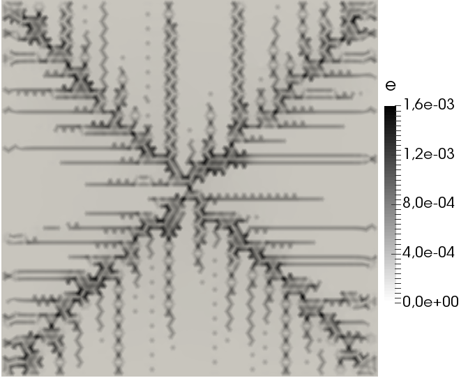 Figure 1
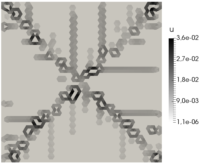 Figure 2
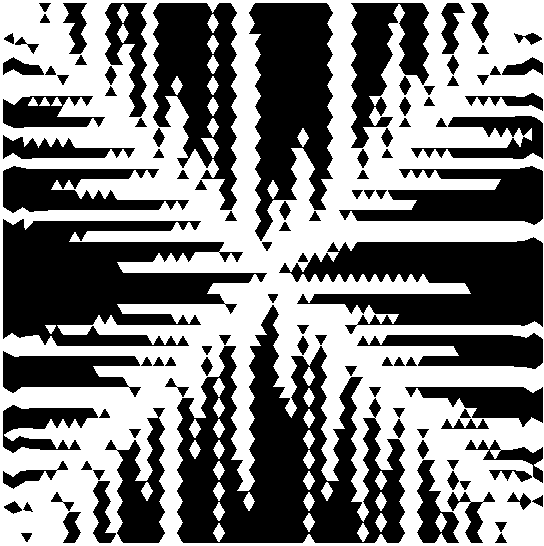 Figure 3
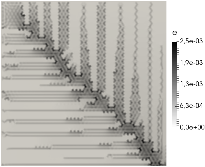 Figure 4
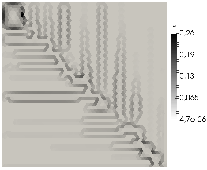 Figure 5
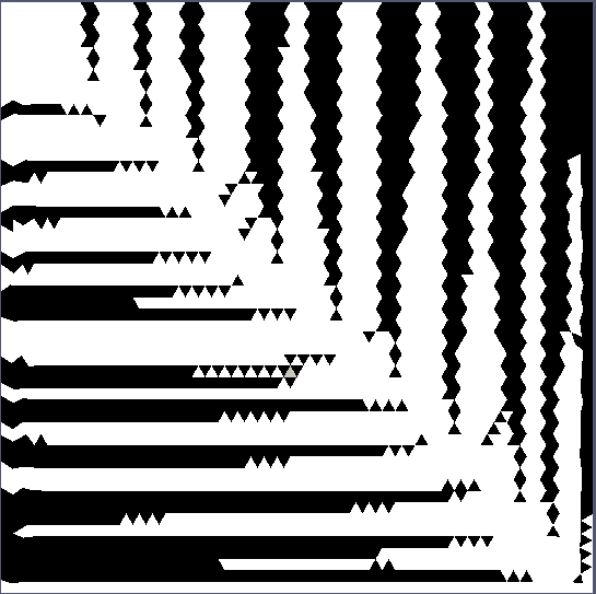 Figure 6
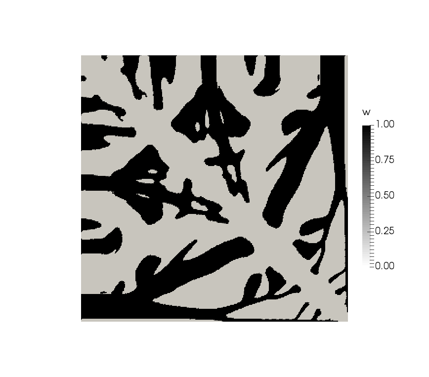 Figure 7
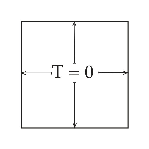 Figure 8
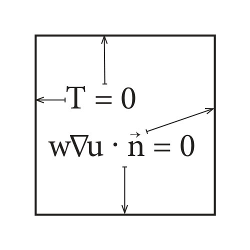 Figure 9
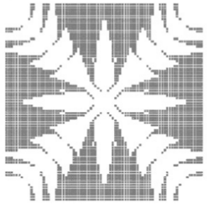 Figure 10
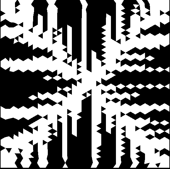 Figure 11
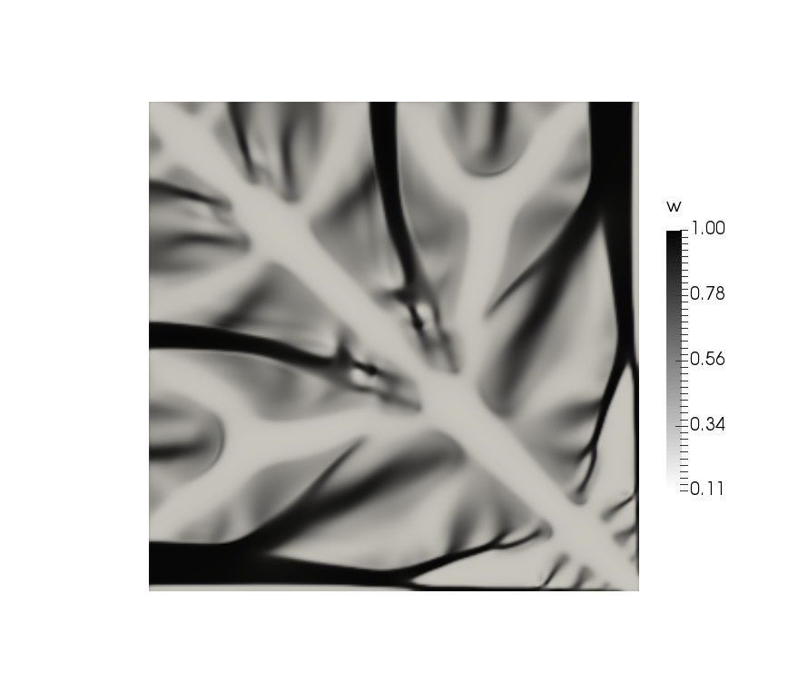 Figure 12
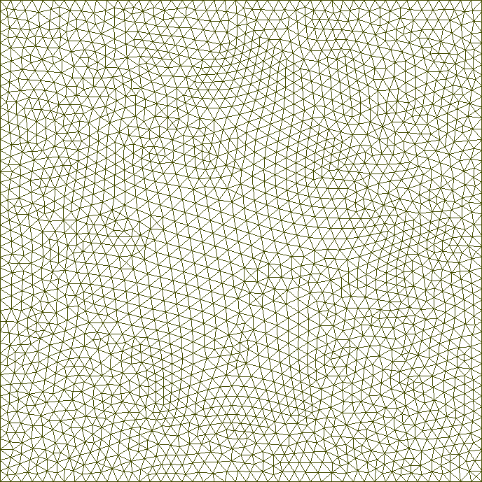 Figure 13
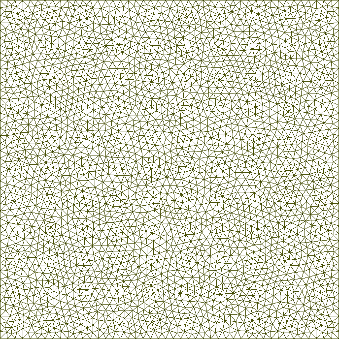 Figure 14
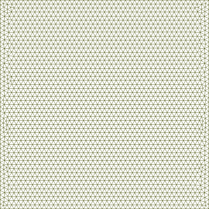 Figure 15
Peer Reviews
No public reviews on file for this paper yet. If you reviewed it on a platform where reviews are public (OpenReview, ICLR, NeurIPS, ICML), you can paste yours below so the community can read it here.
Videos
No videos yet. Explain this paper in a talk, walkthrough, or lecture? Add one.
Taxonomy
TopicsTopology Optimization in Engineering · Advanced Multi-Objective Optimization Algorithms · Composite Structure Analysis and Optimization
Robust regularization of topology optimization problems with aposteriori error estimators
G. V. Ovchinnikov
,
D. Zorin
and
I. V. Oseledets
Abstract.
Topological optimization finds a material density distribution minimizing a functional of the solution of a partial differential equation (PDE), subject to a set of constraints (typically, a bound on the volume or mass of the material).
Using a finite elements discretization (FEM) of the PDE and functional we obtain an integer programming problem. Due to approximation error of FEM discretization, optimization problem becomes mesh-depended and possess false, physically inadequate optimums, while functional value heavily depends on fineness of discretization scheme used to compute it. To alleviate this problem, we propose regularization of given functional by error estimate of FEM discretization. This regularization provides robustness of solutions and improves obtained functional values as well.
While the idea is broadly applicable, in this paper we apply our method to the heat conduction optimization. This type of problems are of practical importance in design of heat conduction channels, heat sinks and other types of heat guides.
Keywords: Topological optimization, greedy methods, finite element methods, error estimators, regularization.
1. Introduction
Topology optimization methods aim to find a material distribution in a volume that minimizes a functional depending on the solution of a PDE describing a physical process, e.g., elastic deformation, heat distribution or electrical current flow.
As in general these problems are noncovex, and even non-smooth, most methods can be viewed as heuristics and do not guarantee reaching a global or local optimum. The solutions produced by commonly used techniques may exhibit substantial mesh dependence with significant difference in functional values obtained for different mesh resolutions, often due to non-physical solutions (“checkerboards”). These solutions are eliminated by different types of regularization techniques, penalizing non-smoothness of the solutions.
While some mesh dependence is unavoidable for discretized problems, we observe that undesirable mesh-dependent solutions are the ones for which the FEM discretization does not yield an accurate estimate of the functional. Informally, the less “smooth”, in the sense of presence of rapid oscillations, the discrete solutions is, the larger is the range of functional values that can be attained by functions agreeing with the discrete solution at sample points.
This view suggests the following idea for regularization: instead of choosing a measure of smoothness a priori, we directly include an estimate of the range of possible functional values in the regularized functional, by adding a term corresponding to the FEM error. While the approximation error can not be measured directly, computable upper bounds are typically available. Thus, instead of minimizing the value of the discretized functional, we minimize the upper bound of the true functional.
More specifically, we use aposteriori estimates to modify the original functionals. This allows us to perform topological optimization using standard sensitivity-based greedy algorithms using a fixed (non-adaptive) discretization. which is important for efficient implementation of the method (including much simpler parallelization).
To summarize, our approach consists of the following elements:
- •
We propose using a posteriori error estimators as reliable regularizers for topological optimization.
- •
We obtain a weak FEM problem formulation to compute the sensitivity of our regularized functionals which can be solved efficiently using a standard FEM solver;
- •
We describe a greedy optimization algorithm based on the computed sensitivity to compute the optimal topology.
- •
For two model problems, we obtained new configurations that have significantlylower functional values that the configurations reported in the literature.
Although we focus on a particular model problem in heat transfer, our approach can be easily generalized to other topology optimization settings.
We start with the description of the method (Sections 2-5) and then compare it to closely related methods and discuss its relationship to most common topology optimization techniques (Section 6,7).
2. Continuous problem
As a model problem in this paper we consider the steady heat conduction problem:
[TABLE]
where is a bounded region with a sufficiently smooth boundary , is in the set of piecewise-continuous functions, which we denote , , and we search for , where is the Sobolev space of functions with zero trace (due to the boundary conditions).
We solve a two-material optimization problem, i.e., is allowed to take only two values: (corresponding to the main material) and (corresponding to the filler material), with being the ratio of conductivity of filler material to that of main material. Our model topology optimization problem is formulated as follows: find a material distribution such that
[TABLE]
A physical interpretation of this optimization problem is the design of optimal heat-conducting device, producing least amount of heat when amount of high-conductivity material is limited. The same mathematical formulations appears not only in heat conduction problems, but also in electrostatic problems [1] or modelling of amoeboid organism growing towards food sources [2].
Note that in general, the problem does not have an optimal solution in ; regularized versions of the problem however, may have sufficiently smooth solutions. The analysis of existence and smoothness of solutions of the optimization problem is beyond the scope of this paper.
3. Discretization
A common way to solve problem (1) is to introduce in a mesh , consisting of elements , and replace by its projection to the finite-dimensional space of functions , which are piecewise constant on the elements:
[TABLE]
where is number of mesh cells and is 1 on -th cell, and zero otherwise. Problem (1) can be written in the following variational form:
[TABLE]
where is a bilinear form on and is a linear functional on dual space:
[TABLE]
We obtain finite element discretization by replacing in (3) by a suitable finite-dimensional space . This leads us to the following system of linear equations for :
[TABLE]
From now on, we will assume is a function for which .
The optimization problem (2) is then approximated by the following integer programming problem:
[TABLE]
The solutions to the discretized problem may exhibit spurious behavior, becoming increasingly oscillatory, with non-physical “checkerboard” patterns emerging, with oscillations on the scale of mesh elements. The emergence of these patterns in the case of elasticity is attributed to the fact that on the scale of the mesh, the discretization exhibit artificial stiffness resulting in a significant underestimation of the functional value. We propose a new way of tackling this type of problems by introducing an additional term into the functional that penalizes that give rises to large errors in the solution.
4. A posteriori error estimators as regularizers
Transition from the initial optimization problem (2) to its discrete counterpart (5) introduces a discretization error, which can be estimated from above as
[TABLE]
The major contribution of this paper is in consideration of the following regularized functional:
[TABLE]
where the regularization term is an upper bound for the error of solution given by . We assume that for some it provides an upper bound for the true functional:
[TABLE]
Our idea is to minimize the upper bound , instead of the discretization of the functional itself. While the value of for the resulting solution may be larger, one can guarantee that is not arbitrarily large, unlike the case of standard greedy methods, which may lead to solutions for which can be significantly larger than .
There are many ways to introduce the regularizer term based on the error estimation; we present a simple error estimator bounding the squared error:
[TABLE]
to ensure that the regularized functional is differentiable everywhere. We obtain a simple regularizer from from the following variational form [3]. Let , then
[TABLE]
For Galerkin discretizations, the error is orthogonal to , and hence we need to choose subspace to solve for the error:
[TABLE]
Choosing leads us to the regularized version of (5):
[TABLE]
5. Optimization problem
5.1. Greedy optimization
To solve (5) we use the approach that has been successfully used in the topology optimization: the greedy “hard-kill” methods introduced in [4], [5] and [6], and used more recently in [7]). Those methods remove/add a whole patch of material on each step, in contrast to the “soft-kill” methods which evolve a smooth material density function which is discretized in the final step by thresholding and/or filtering. One can easily see that both continuous and discrete functionals and are monotonous with respect to changes in , so “removing material” (i.e., replacing by ) always increases it, because boundary conditions are chosen such that to be non-negative. The greedy approach to solving this problem removes the material from an element that results in least change to the functional. To estimate the change in the functional, we use its sensitivity, i.e., the derivative of the functional with respect to the coefficient of the material distribution corresponding to the -th element:
[TABLE]
An efficient way to compute sensitivities will be described in Section 5.2 Algorithm 1 summarizes the complete method.
For a given problem we can vary the number of elements and mesh connectivity, which affects the material distribution and functional value. We will discuss the effects of those parameters in numerical experiments section 6.2.1.
5.2. Computing sensitivity
The derivatives of the regularized functional consists of two terms, corresponding to the original functional and the regularization term. The expression for the former is well-known (we provide the derivation for the sake of completeness); we derive the expression for the regularizer.
We represent the form in finite-dimensional spaces and by symmetric stiffness matrices and : , and , which leads us to the following equations for and :
[TABLE]
[TABLE]
We use the same notation for functions and their coefficient vectors, as the difference is clear from the context (the coefficient vectors are used only in matrix equations).
Matrices and project a function in to a function in and vice versa. To simplify derivation, for the rest of the paper, we assume that and , for example being generated by the same basis function family, but on finer mesh, hence is the inclusion operator.
The discretized unregularized functional can be written as ; Using , where is independent of , we obtain
[TABLE]
From it follows
[TABLE]
We conclude that
[TABLE]
5.2.1. Sensitivity of the regularization term
Now, we have two natural choices for error estimate from (8). First, , and second, .
Theorem 1**.**
Sensitivity of the functional regularized by is
[TABLE]
Sensitivity of the functional regularized by is
[TABLE]
Proof.
The first part of the formulas is given by (12). For the second part, notice that from (10) and (11) follows:
[TABLE]
Then sensitivity of can be written as
[TABLE]
and hence
[TABLE]
This, combined with (12) proves (13). Now, consider :
[TABLE]
Then sensitivity of can be written as
[TABLE]
and hence
[TABLE]
This, combined with (12) proves (14).
∎
5.3. Computational details
To compute , and observe that
[TABLE]
[TABLE]
Using these expressions we compute sensitivities by solving for and using a FEM solver, computing their gradients, and then compute integrals (15) and (16). If an optimal-complexity linear solver is used (e.g., multigrid) the overall cost of the computation is linear in the total number of elements in and .
6. Numerical experiments
6.1. Test cases
Although topology optimization by greedy methods has been studied extensively, there are relatively few papers considering topology optimization for heat conduction. We use [7] and [8] for comparison purposes.
We consider two model 2D problems, both of each have been studied in literature, which allows us to provide comparisons with other methods: problem A was considered in [8] and Problem B in [9] and [7].
Both problems are formulated on a simple square domain of size 1, and a uniform heat distribution with unit density is assumed.
Problem A. For this problem, Dirichlet boundary conditions are specified on two boundary segments and Neumann conditions on the other two (Figure 1, left). The target volume fraction occupied by the material for this problem is set to , to be consistent with [8].
Problem B. For this problem, Dirichlet conditions are specified on the whole boundary (Figure 1), and the target volume fraction occupied by the material for this problem is set to , following [9] and [7].
Our main comparison measure is the relative increase in the functional value
[TABLE]
where is the value of the functional corresponding to the whole domain filled with material, i.e., for all elements. Since the functional always increases with the removal of the material, the smaller this number is, the better is the result.
6.2. Implementation
We implemented Algorithm 1 using FireDrake finite element solver ([10], [11], [12], [13]). We use the regularized functional (6) and expressions for sensitivities (15), (16). While for numerical experiments we consider only squares, the approach, obviously, works for arbitrary sufficiently regular geometry (the problem must be solvable with FEM, obviously) both in 2D and 3D.
For our experiments we choose to be the standard space of piecewise-linear continuous functions on triangular mesh; is represented by piecewise-constant functions on triangles. The space needed for the error bound is also the space of piecewise-linear continuous functions on the mesh which is a uniformly refined version of original mesh . In the experiments we use three different meshes generated by GMSH [14] (Figure 2). Also, since we don’t need regularizer to be very precise for simplicity of implementation we used
[TABLE]
as compromise between (13) and (14) which does not require projections.
6.2.1. Dependence on regularization parameter and mesh-dependence
We first explore the dependence of the final functional value on the regularization parameter , in the range from until . Simultaneously, we explore the mesh dependence of the method by running Algorithm 1 on all combinations of meshes and regularization parameters.
As evident from the Figure 3, there is a noticeable dependence on the mesh choice at this resolution; At the same time, it is also clear that the method is relatively insensitive to the choice of , as long as it is sufficiently large: and the effects of the choice of are not mesh-dependent, and are similar for both problems.
Observe that the optimal values of are large: effectively, minimization of the error needs to be prioritized over minimizing the discrete functional value for best results. Intuitively, one can interpret this as searching for optimal designs in the constrained space of functions minimizing the error on a finer mesh. As evident from Figure 4 functional converges with respect to mesh size very fast, with only one level of refinement sufficient.
6.3. Problem A
Based on the results shown in Figure 3, we use in the remaining experiments. The material distribution found by our algorithm can be seen in Figure 5, (c). The obtained material distribution features thin heat-sink channels, similar to the ones from solutions of other authors.
A fundamental difference between our method and the method of [8] is that we solve the problem with discrete material values directly, while [8] solves a relaxation of the problem with a continuous material distribution. This approach has significant advantages as, due to convexity [15], such problems are easier to solve. In addition, by searching a larger space of material distributions, lower values of the functional can be obtained. However, as in practice creating continuous material variation is typically difficult or impossible, a final thresholding step needs to be applied, which typically leads to a significant increase in the functional.
Our solution appears to be less fractal than solution from [8]. Note that [8] considers continuous optimization problem, as material density allowed to be in .
Aggregated results for Problem A are shown in Table 1:
[TABLE]
6.4. Problem B
Solution of this optimization problem features the same thin heat-sink channels as with problem A. Our solution looks different from solution of [7], which presents smaller number of larger channels with fractal-like border. On the other hand, our solution propose more thin channels with relatively smooth borders. The jigsaw borders of heat sinks are due to mesh effects (compare smoother borders of the channels in top and bottom versus rougher borders of the channels in left and right). The comparison results are shown in Table 2.
[TABLE]
7. Discussion and related work
7.1. Previous approaches to regularization
Regularization techniques were used in topological optimization primarily to solve two problems: to avoid formation of spurious solutions (checkerboard patterns) and to remove mesh dependency. Regularization was applied in the context of all commonly used approaches to topology optimization: density-based, hard-kill and level set/phase-field methods.
Most regularization approaches can be roughly divided into two groups: filtering methods and constraint techniques [17].
There are several types of filtering methods: the two most widely used types are density filters which directly modify the solution ([18], [19]), and sensitivity filters ([20], [16]). Recently filtering methods based on the Helmholtz equation were applied to both sensitivity and material density ([21], [22]). Another recent development is the design of density filters which are based on projection schemes. Those methods operate on density field , its filtered version and a projected field . Most filtering methods result in continuous density distributions, which need to be thresholded in the context of hard-kill methods, the projection methods reported to have good convergence and almost discrete designs ([23], [24], [25], [26], [27]).
Constraint methods modify optimization problem by imposing a constraint either as hard constraint, or via a penalty term in the objective functional. A common type constrained quantity is an integral of the form
[TABLE]
i.e., a -norm of the gradient. E.g., leads to the total variation constraint or penalty [28], [29], results in the usual gradient norm (Dirichlet energy) and yields a pointwise constraint on the gradient magnitude [30], [31]. In [32], proposed a similar penalty based on density discrepancy. Regularization for level-set methods can be found, e.g., in [33], where the primary goal of regularization is to smooth the velocity field and maintain smoothness of the level set. Detailed reviews of relevant literature can be found in two excellent surveys: [17] and [34].
In contrast to most previous methods, our approach aims to use regularization to control the error of the FEM solution directly, and in this way, increase robustness of the method, by potentially increasing the value of the discretized functional for the solution, but ensuring that it does not deviate too much from the underlying smooth functional.
Our experiments demonstrate however, that in the context of hard-kill methods, this regularization actually results in a decrease of the (unregularized) functional value. This happens because approximation error introduced by finite elements methods creates false minimums for objective functional. First, greedy methods will likely to get stuck in those minimums. Second those false minimums depend on mesh and result in growth of functional on different or refined mesh. Regularization removes those false minimums and mesh dependence, making functional value being closer to its true physical value.
8. Conclusions and future work
Greedy methods based on sensitivity analysis are popular due to their ease of implementation on top of existing FEM packages. On the downside, the integer programming problems resulted from discretization are complex, and the convergence behavior is often unpredictable.
In our experiments we have demonstrated that our regularization applied to “hard-kill” method allows it achieve results close to those of a density-based method from [8], and a significant improvement compared to a previously proposed “hard-kill” method [7], with the functional value two times less.
The estimator used to regularize our functional requires additional finer mesh and solution of additional problem on that mesh. Although it is very easy to implement, this incurs an additional cost. In the future, we will explore regularization with a more efficient (e.g., adaptive) error estimator, along with applications of approach proposed in this paper to topology optimization in the context of elasticity as well as to 3D problems.
The reference list from the paper itself. Each links out to its DOI / PubMed record.
- 1[1] G. Steven, Q. Li, Y. Xie, Evolutionary topology and shape design for general physical field problems, Computational mechanics 26 (2) (2000) 129–139.
- 2[2] A. Safonov, J. Jones, Physarum computing and topology optimisation, International Journal of Parallel, Emergent and Distributed Systems 0 (0) (2016) 1–18. doi:10.1080/17445760.2016.1221073.
- 3[3] T. Grätsch, K.-J. Bathe, A posteriori error estimation techniques in practical finite element analysis, Computers & structures 83 (4) (2005) 235–265.
- 4[4] Y. M. Xie, G. P. Steven, A simple evolutionary procedure for structural optimization, Computers & structures 49 (5) (1993) 885–896.
- 5[5] Y. M. Xie, G. P. Steven, Basic evolutionary structural optimization, Springer, 1997.
- 6[6] O. Querin, G. Steven, Y. Xie, Evolutionary structural optimisation (eso) using a bidirectional algorithm, Engineering Computations 15 (8) (1998) 1031–1048.
- 7[7] T. Gao, W. Zhang, J. Zhu, Y. Xu, D. Bassir, Topology optimization of heat conduction problem involving design-dependent heat load effect, Finite Elements in Analysis and Design 44 (14) (2008) 805–813.
- 8[8] A. Gersborg-Hansen, M. P. Bendsøe, O. Sigmund, Topology optimization of heat conduction problems using the finite volume method, Structural and multidisciplinary optimization 31 (4) (2006) 251–259.