Periodic quantum graphs from the Bethe-Sommerfeld perspective
Pavel Exner, Ond\v{r}ej Turek

TL;DR
This paper investigates the spectral gap properties of periodic quantum graphs, proving the impossibility of the Bethe-Sommerfeld property under certain conditions and constructing explicit examples with a finite number of gaps.
Contribution
It establishes conditions under which quantum graphs cannot have finitely many gaps and provides explicit constructions of graphs with any prescribed finite number of spectral gaps.
Findings
Quantum graphs with scale-invariant vertex couplings cannot have the Bethe-Sommerfeld property.
Explicit examples of quantum graphs with any finite number of spectral gaps are constructed.
Demonstrates the existence of quantum graphs with a prescribed finite number of spectral gaps.
Abstract
The paper is concerned with the number of open gaps in spectra of periodic quantum graphs. The well-known conjecture by Bethe and Sommerfeld (1933) says that the number of open spectral gaps for a system periodic in more than one direction is finite. To the date its validity is established for numerous systems, however, it is known that quantum graphs do not comply with this law as their spectra have typically infinitely many gaps, or no gaps at all. These facts gave rise to the question about the existence of quantum graphs with the `Bethe-Sommerfeld property', that is, featuring a nonzero finite number of gaps in the spectrum. In this paper we prove that the said property is impossible for graphs with the vertex couplings which are either scale-invariant or associated to scale-invariant ones in a particular way. On the other hand, we demonstrate that quantum graphs with a finite…
Click any figure to enlarge with its caption.
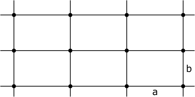 Figure 1
Peer Reviews
No public reviews on file for this paper yet. If you reviewed it on a platform where reviews are public (OpenReview, ICLR, NeurIPS, ICML), you can paste yours below so the community can read it here.
Videos
No videos yet. Explain this paper in a talk, walkthrough, or lecture? Add one.
Periodic quantum graphs from the Bethe–Sommerfeld perspective
Pavel Exner1,2, Ondřej Turek2,3,4
1 Doppler Institute for Mathematical Physics and Applied Mathematics, Czech Technical University in Prague, Břehová 7, 11519 Prague, Czech Republic
2 Department of Theoretical Physics, Nuclear Physics Institute CAS, 25068 Řež near Prague, Czech Republic
3 Bogoliubov Laboratory of Theoretical Physics, Joint Institute for Nuclear Research, 141980 Dubna, Russian Federation
4 Laboratory for Unified Quantum Devices, Kochi University of Technology, 782-8502 Kochi, Japan
[email protected], [email protected]
Abstract
The paper is concerned with the number of open gaps in spectra of periodic quantum graphs. The well-known conjecture by Bethe and Sommerfeld (1933) says that the number of open spectral gaps for a system periodic in more than one direction is finite. To the date its validity is established for numerous systems, however, it is known that quantum graphs do not comply with this law as their spectra have typically infinitely many gaps, or no gaps at all. These facts gave rise to the question about the existence of quantum graphs with the ‘Bethe–Sommerfeld property’, that is, featuring a nonzero finite number of gaps in the spectrum. In this paper we prove that the said property is impossible for graphs with the vertex couplings which are either scale-invariant or associated to scale-invariant ones in a particular way. On the other hand, we demonstrate that quantum graphs with a finite number of open gaps do indeed exist. We illustrate this phenomenon on an example of a rectangular lattice with a coupling at the vertices and a suitable irrational ratio of the edges. Our result allows to find explicitly a quantum graph with any prescribed exact number of gaps, which is the first such example to the date.
pacs:
02.30.Tb, 03.65.Nk, 03.65.Db
††: J. Phys. A: Math. Gen.
Keywords: quantum graphs, periodic structure, Bethe–Sommerfeld conjecture, vertex coupling, Diophantine approximation
1 Introduction
Quantum graphs are one of the fast developing areas of quantum physics, the interest to them being driven both by their ‘practical’ use in modeling nanostructures and other physical objects, as well as by theoretical reasons. They allow us to understand better various quantum effects by analyzing them in the situation where the configuration space has nontrivial geometrical and topological properties. The literature concerning quantum graphs is extensive and we limit ourselves to referring the reader to the recent monograph [4] as a guide to further ilumination.
While the quantum graph Hamiltonians describing particles ‘living’ on a metric graph share many properties with the ‘usual’ Schrödinger operators, this analogy is far from being complete; a well-known example is the failure of the unique continuation property [4, Sec. 3.4] that makes possible, for instance, the existence of compactly supported eigenfunctions on infinite graphs. This concerns, in particular, infinite periodic graphs the spectrum of which may not be purely absolutely continuous containing flat bands, or infinitely degenerate eigenvalues, and it is even possible that the absolutely continuous part is empty as is the case for magnetic chain graphs with a half-of-the-quantum flux through each chain element [12, Thm. 2.3].
Our goal in this paper is to investigate Hamiltonians of infinite periodic graphs from another point of view, namely the number of open gaps in their spectra. To begin with we recall the Bethe–Sommerfeld conjecture [23] put forward in the early days of the quantum theory, according to which a quantum system periodic in more than one direction — with a slight abuse of terminology one usually speaks of -periodicity with — has a finite number of open gaps in the spectrum only. The reasoning behind the conjecture is based on the behavior of the spectral bands identified with the ranges of the dispersion curves or surfaces. Those at most touch for -periodic systems while in higher dimensions they typically overlap making opening of gaps more and more difficult as we proceed to higher energies. This looked convincing and the property was taken for granted, although mathematically it proved to be a rather hard problem and it took decades before an affirmative answer was obtained for most cases of the ‘ordinary’ Schrödinger operators — see, for instance, [8, 13, 17, 21, 22] and references therein.
Discussing this question in the context of quantum graphs, the authors of [4] recall the above mentioned heuristic argument (Sec. 4.7), however, they add immediately that this is not a ‘strict law’; in Sec. 5.1 of [4] they illustrate this claim by examples of periodic graphs with an infinite number of resonant gaps created by a graph ‘decoration’, the effect noticed first in the context of discrete graphs [19] and later verified also for metric graphs111Cf. [16] and [4, Sec. 5.1] for more details. Let us add that decorations can produce an infinite number of spectral gaps also in systems that are -periodic only [1].. In other words, we have examples of numerous situations in which the claim represented by the BS conjecture is false. The question thus arise whether it is a ‘law’ at all, that is, whether there are infinite periodic graphs having a finite nonzero number of open gaps above the threshold of the spectrum. This is the topic we are going to discuss in the present paper; for the brevity of expression we will speak of those graphs as of graphs belonging to the Bethe–Sommerfeld class, or simply Bethe–Sommerfeld graphs.
We have two main conclusions. The first one concerns the fact that the said property is sensitive to the type of vertex coupling. Recall that the general self-adjoint coupling condition, commonly written as , can be decomposed into the Dirichlet, Neumann, and Robin parts [4, Thm. 1.4.4]; if the latter is absent we call such a coupling scale-invariant.
Theorem 1.1**.**
An infinite periodic quantum graph does not belong to the Bethe–Sommerfeld class if all the couplings at its vertices are scale-invariant.
In fact, one can make a stronger claim. Given a graph with general couplings we consider the same graph with the couplings made scale-invariant by removing the Robin component in the way described in Section 2.3. Comparing their spectra, we find:
Theorem 1.2**.**
If an infinite periodic quantum graph with scale-invariant couplings at the vertices has at least one open gap, then adding a Robin component to the couplings cannot produce a Bethe–Sommerfeld graph.
On the other hand, we are going to demonstrate that the said class is nonempty. Our second main result in this paper is expressed in the following claim.
Theorem 1.3**.**
Bethe–Sommerfeld graphs exist.
As it is usually the case with existence claims it is sufficient to present an example. With this aim we revisit in the second part of the paper the model introduced in [9] and further discussed in [10, 11] describing a periodic lattice whose basic cell is a rectangle of the side ratio and the coupling in the vertices is of the -type with a coupling constant . It was shown in the mentioned papers that the spectral properties of such a quantum graph depend on the number-theoretical properties of the ratio . Here we are going to demonstrate that if is badly approximable by rationals, there are values of for which this graph belongs to the Bethe–Sommerfeld class. More than that, our construction makes it possible to find values of for which the lattice graph in question has any prescribed number of gaps.
Before closing the introduction, let us recall that there are examples of the ‘usual’ Schrödinger operators where the question about validity of the conjecture remains open, a prominent example being Laplacian in a periodically curved tube or a Schrödinger operator in a straight tube with a -periodic potential. These systems are sometimes said to have a ‘mixed dimensionality’ even if they are obviously periodic in one direction only, however they have a ‘two-dimensional’ feature, namely that in the absence of potential or the deformation they have intersecting dispersion curves, which could suggest a BS-type behaviour. An analogue of such systems in the present context are -periodic graphs with period cells connected by more than a single link for which the question about the Bethe-Sommerfeld property remains also open; note that Theorems 1.1 and 1.2 apply to such graphs.
2 Absence of the Bethe–Sommerfeld property
In this section we are going to prove Theorems 1.1 and 1.2.
2.1 The ST-form of the coupling
As it is common in the quantum graph theory the Hamiltonians we consider act as the (negative) second derivative on the graph edges with the domain consisting of functions which belong locally to the second Sobolev space and satisfy suitable coupling conditions at the vertices. For the purposes of the argument it is useful to write the vertex conditions, instead of the commonly used way mentioned in the introduction, in the so-called ST-form proposed in [6]. Given a vertex of degree , the vectors and in will again stand for the boundary values in the vertex,
[TABLE]
where the limits of the first derivatives are conventionally taken in the outward direction. The coupling condition at the vertex can be then written as
[TABLE]
for certain , , and , where the symbol denotes the identity matrix of order and the matrix is Hermitian. The condition (2.1) allows us to single out scale-invariant couplings; it is easy to see that the coupling has this property if and only if [7]. In particular, the on-shell scattering matrix for the vertex in question is in the -formalism given by
[TABLE]
and it is obvious that is independent of iff .
The spectrum is obtained using the Bloch-Floquet theory. The way to do that is well known, cf. [4, Sec. 4.2] and references therein, we describe it nevertheless briefly here to make the paper self-contained. We assume that the graph is locally finite and consider its elementary cell; cutting it out from the original periodic graph we get a finite family of pairs of ‘antipodal’ vertices related mutually by the action of the corresponding translation group. Each such pair of vertices can be regarded as a single vertex with the boundary conditions
[TABLE]
for some , where , and is the dimension of translation group associated with graph periodicity. The pair of edges with the endpoints can be turned into a single edge by identifying these endpoints, and the acquired phase coming from the conditions (2.3) can be also regarded as being induced by a magnetic potential. Let us denote the graph obtained in this way from the elementary cell by , and the number of its edges by . Regarding each edge of as a pair of two directed edges (bonds) of opposite orientations and indexing the bonds by , we consider the matrices , and which are defined in the following way. The matrix is a diagonal matrix whose -th diagonal entry is the length of the -th bond. The diagonal matrix has the entries and at the pair of the diagonal positions corresponding to the -th edge of created by the mentioned vertex identification; all its other entries are zero. Finally, the matrix is the bond scattering matrix, which contains directed edge-to-edge scattering coefficients. In this way, each element of the matrix corresponds to a certain entry of the scattering matrix at a certain vertex of the elementary cell, cf. [4, eq. (2.1.15)]. Recall that the bond scattering matrix is unitary. Having introduced the matrices , , and , we define the function as
[TABLE]
this allows us to write the spectral condition in the form
[TABLE]
Note that the function is in general complex, however, one can consider a real-valued function instead, dividing by , cf. [4, Rem. 2.1.10].
2.2 Graphs with scale-invariant couplings
As we have indicated, the described way of treating periodic quantum graphs is pretty standard. It has an important advantage, namely that it allows one to analyze properties of the ergodic flow on the torus associated with such a system. This idea can be traced back to Barra and Gaspard [3] and it was recently used by Band and Berkolaiko [2] to derive a deep result about spectral universality for periodic quantum graphs with the simplest vertex coupling, usually referred to as Kirchhoff or Neumann. We are going to use an argument analogous to that of [2] in Proposition 2.2 below.
Consider first the case of a periodic graph with scale-invariant couplings at all the vertices. The scale-invariance assumption implies that the scattering matrix at each graph vertex is independent of and the same is naturally true for the matrix entering formula (2.4). From now on, let denote the left hand side of formula (2.4) for a graph with scale-invariant couplings. The function value thus depends on the vectors and , where , is the set of mutually different edge lengths of . Moreover, the value is -periodic in each of the terms . Let us define
[TABLE]
where the symbol stands for the difference between and the nearest integer multiple of , i.e.
[TABLE]
Since the value depends on the vectors and only, it is convenient to introduce a function
[TABLE]
and write the spectral condition (2.5) in the form
[TABLE]
Lemma 2.1**.**
Let be given by (2.6). For any , and there is a such that .
Proof.
We shall prove that
[TABLE]
where the symbol was defined in (2.7). We will use the simultaneous version of the Dirichlet’s approximation theorem. First of all, we set
[TABLE]
for all . The said theorem guarantees for any and for any natural number the existence of integers , , such that
[TABLE]
Let , and be given and choose as an integer with the property that
[TABLE]
Once is fixed, the number can be taken as any integer satisfying
[TABLE]
Let be the integer from the simultaneous version of the Dirichlet’s approximation theorem corresponding to chosen according to (2.14). Notice that depends on , and therefore also on . For this , we define as follows,
[TABLE]
Our aim is to show that satisfies the following two conditions:
[TABLE]
Applying the definition of , the inequality and the assumption (2.13), we get
[TABLE]
in other words, condition (2.15) holds true. Let us proceed to condition (2.16). We have
[TABLE]
where was introduced in equation (2.11). Since holds obviously for all and , we obtain in particular
[TABLE]
for denoting the integers from (2.12). Consequently, the inequality (2.12) and the assumption (2.14) imply
[TABLE]
which proves condition (2.16). The claim (2.10) thus holds true. ∎
Proposition 2.2**.**
Let be a Hamiltonian of a periodic quantum graph with scale-invariant couplings at all the vertices. Then the following holds:
- (i)
If contains a gap, then it contains infinitely many gaps.
- (ii)
Furthermore, if has a gap of size in terms of momentum, then for every there is an infinite sequence of gaps of sizes at least (in terms of momentum).
- (iii)
In particular, if all the graph edge lengths are rationally dependent, then the momentum spectrum is periodic.
Proof.
The claim (i) is obviously a straighforward consequence of (ii). To prove (ii), let us assume that has a gap of size in terms of , i.e., there is a such that for all . According to (2.9), the gap condition reads
[TABLE]
Since is a continuous function, it attains minimum on any compact interval. In particular, for any given there exists the minimum
[TABLE]
The value is positive, because all values in the interval \bigl{[}k_{0}-\frac{s-\epsilon}{2},k_{0}+\frac{s-\epsilon}{2}\bigr{]} correspond to a gap. Moreover, the Brillouin zone has the structure of a torus, hence the function is periodic with the period in every component of the vector , which in particular means that the same value of minimum is attained also at the left-open interval . Hence we obtain
[TABLE]
Now we use Lemma 2.1, which guarantees that for every one can find a such that for all , the quantity \big{|}\left\{k^{\prime}\ell_{j}-k\ell_{j}\right\}_{(2\pi)}\big{|} is as small as required. With regard to a trivial identity for , also the quantity \bigl{|}\left\{(k^{\prime}+x)\ell_{j}-(k+x)\ell_{j}\right\}_{(2\pi)}\bigr{|} can be as small as required for all . This fact together with the continuity of implies that for every given , one can find a with the property
[TABLE]
Now we apply the triangle inequality together with (2.18) and (2.19) to obtain the estimate
[TABLE]
for all and . To sum up, for any one can find a such that for all . This proves the existence of infinitely many gaps of sizes at least in terms of , given the fact that the operator in question is unbounded and the resolvent set of is open.
It remains to prove (iii). If all the lengths are rationally dependent, there exists an elementary length and integers such that holds for . Hence which implies
[TABLE]
for all . This means that is periodic with period , and consequently, the spectrum has a periodic structure in terms of the momentum. ∎
Corollary 2.3**.**
Theorem 1.1 is valid.
2.3 The case of general vertex couplings
Our next aim is to show that the Bethe–Sommerfeld property can be excluded also for graphs with vertex couplings from a wider class. We begin with the following definition.
Definition 2.4**.**
Let a vertex coupling be given by condition (2.1). The associated scale-invariant vertex coupling is given by condition
[TABLE]
In other words, the coupling associated to a given (2.1) is obtained by removing the Robin part represented by the square matrix .
In the following proposition we show that the scattering matrix referring to (2.1) decomposes into a constant part and a part that vanishes as . This observation is useful for dealing with high momenta values, , note that this is the regime crucial from the viewpoint of the Bethe–Sommerfeld property.
Proposition 2.5**.**
Consider a quantum graph vertex with a general coupling described by the condition (2.1). Its scattering matrix satisfies
[TABLE]
where
[TABLE]
is the constant scattering matrix corresponding to the associated scale-invariant vertex coupling (2.20), and
[TABLE]
Moreover, the matrix function is bounded on the interval .
Proof.
The scattering matrix obeys equation (2.2). Using the identity
[TABLE]
we obtain (2.21) for and given by (2.22) and (2.23), respectively. Finally, the boundedness of on is a straightforward consequence of the continuity of and the existence of the limit
[TABLE]
∎
Each entry of the matrix , appearing in (2.4), is equal by definition to a certain entry of for some vertex of . Therefore, Proposition 2.5 allows us to decompose the matrix in a way similar to (2.21),
[TABLE]
where is a constant unitary matrix, corresponding to the same graph with the associated scale-invariant couplings at its vertices, and is a matrix that is bounded on as a function of .
Proposition 2.6**.**
The quantity of (2.4) can be expressed as
[TABLE]
where
[TABLE]
and the function is continuous and bounded on .
Proof.
According to (2.24) we have
[TABLE]
with and . The expansion of takes the form , where is a sum of products of entries of the matrices and multiplied by non-negative powers of . Since the entries of and are continuous and bounded on (cf. (2.24)), the function has the same property. ∎
Theorem 2.7**.**
Consider a periodic graph with general couplings at the vertices and denote its spectrum as . Let further be the spectrum of the same graph, in which all vertex couplings are replaced by the associated scale-invariant couplings. Then the following claims hold true:
- (i)
If has an open gap, then has infinitely many gaps.
- (ii)
In particular, if has a gap of size in terms of momentum, then for every there are infinitely many gaps of of sizes at least (in terms of momentum).
Proof.
Since (i) is a straightforward consequence of (ii), it suffices to prove (ii). Let have a gap of size in terms of , i.e., let there be a such that for all k\in\bigl{(}k_{0}-\frac{s}{2},k_{0}+\frac{s}{2}\bigr{)}. In the same way as in the proof of Proposition 2.2(ii), one can show that for any , there is a such that
[TABLE]
(cf. (2.18)), and then demonstrate that for any there is a such that
[TABLE]
for all x\in\bigl{[}-\frac{s-\epsilon}{2},\frac{s-\epsilon}{2}\bigr{]} and (cf. (2.19)). Let us limit ourselves to large values , specifically, to the values with the property
[TABLE]
where is the term appearing in equation (2.25). Now we apply twice the triangle inequality to the decomposition (2.25) and after that we use inequalities (2.26), (2.27), and (2.28). In this way we obtain
[TABLE]
for all x\in\bigl{[}-\frac{s-\epsilon}{2},\frac{s-\epsilon}{2}\bigr{]} and . That is, to any sufficiently large one can find a such that for all , which proves the result. ∎
Corollary 2.8**.**
Theorem 1.2 is valid.
Let us finally remark that the gaps of seem to asymptotically coincide with those of , however, we are not going to pursue this question here.
3 Number theoretic preliminaries
Before turning to our second main topic—establishing the existence of Bethe–Sommerfeld graphs—we need to introduce some number-theoretic notions on which the subsequent spectral analysis will rely substantially. A number is called badly approximable if there exists a such that
[TABLE]
for all with . An irrational number is badly approximable if and only if the elements of its continued-fraction representation are bounded [15]. With our goal in mind we note that the badly approximable numbers emerged in [10] as the only ratios for which the spectrum of a rectangular lattice with edges and and couplings in the vertices may have a finite number of gaps.
The so-called Markov constant of is defined as
[TABLE]
with meaning “there exist infinitely many”. The Markov constant is sometimes denoted by , cf. [5]. Notice that if and only if is badly approximable. Since every has trivially , some authors define only for being irrational.
Recall that by a theorem of Hurwitz [14] for every irrational number there are infinitely many such that , in other words, holds for any .
We say that are equivalent if there are integers such that
[TABLE]
According to [5, Thm. IV], are equivalent if and only if their continued fractions take the form
[TABLE]
for suitable and , , and . One can prove that if and are equivalent, then ; cf. [5, p. 11]. The particular choice and in equation (3.2) establishes the equivalence of the numbers and ; hence
[TABLE]
Now we will introduce a function the values of which will play an important role in the analysis of our spectral problem; they can be regarded as a one-sided version of the Markov constant.
Definition 3.1**.**
For any , we set
[TABLE]
Proposition 3.2**.**
*For every , we have *
[TABLE]
where and are the floor and the ceiling function, respectively.
Proof.
One can see easily that the right-hand side of (3.5) will remain unchanged if we assume and is replaced with , i.e.,
[TABLE]
In this way we obtain formula (3.6).
Let us next prove (3.7). It follows from the definition that the left-hand side of (3.7) equals
[TABLE]
At the same time, in analogy with the previous step, it is easy to see that the right-hand side of (3.7) is equal to
[TABLE]
Our goal is to prove that . To that end we will use the identity
[TABLE]
which implies
[TABLE]
hence . At the same time, for every there are infinitely many such that . Therefore, due to identity (3.11), there are infinitely many such that
[TABLE]
Choosing large enough, we can find for any and any infinitely many pairs with the property
[TABLE]
Consequently, we have also the inequality which completes the proof of the sought relation .
It remains to prove formula (3.8). We know from the previous step that according to (3.10), hence
[TABLE]
Formula (3.8) follows trivially from equations (3.5), (3.12) (where we have to rename the variables, , ) and (3.1). ∎
Regarding equation (3.8), let us remark that the values and may or may not coincide. For example, for the golden mean, , we have (see Section 5 below), on the other hand, the literature on the Markov constant provides hints of the existence of numbers with the property , see e.g. [18].
Function is closely related to approximations of by rationals. A number with is called best Diophantine approximation of the second kind to a given if
[TABLE]
holds for all such that and . A is a best Diophantine approximation of the second kind to a if and only if it is a convergent of the continued fraction corresponding to (except for the trivial case , ), see e.g. [15]. Recall that a convergent of a is a rational number equal to a finite initial segment of a continued fraction representation of , e.g., , , , etc. If the inequality (3.13) is replaced with , the corresponding fraction is called best Diophantine approximation of the first kind to the number .
For the discussion of the problem we address in this work, we will need a certain type of one-sided best approximations, which we will call, in analogy to the notions mentioned above, ‘best approximation from below (respectively, from above) of the third kind’. They are defined as follows.
Definition 3.3**.**
Let and for . We say that the number is a best approximation from below of the third kind to if
[TABLE]
for all such that , and . Likewise, we call a best approximation from above of the third kind to if
[TABLE]
for all such that , and .
Notice that for every irrational , there are infinitely many best approximations from below of the third kind to . Let us regard them as a sequence such that grow with . According to Definition 3.3, the corresponding values form a decreasing sequence, the limit of which cannot be less than by (3.5). Furthermore, considering (3.5) and the fact that the approximations are best in terms of (3.14), we have the result
[TABLE]
Formula (3.16) combined with an explicit characterization of the terms , which will be found in Proposition 3.5 below, greatly simplifies the evaluation of the function .
Lemma 3.4**.**
Let and , be convergents of . If the inequalities
[TABLE]
hold, then we have
[TABLE]
Proof.
First we estimate the absolute value from below,
[TABLE]
where we used a trivial fact that because the expression is by assumption a nonzero integer. In the next step we find an upper estimate of the same quantity, taking advantage of a known formula (cf. [15, Cor. of Thm. 3]) for representing the continued-fraction form of ,
[TABLE]
Combining inequalities (3.17) and (3.18), we obtain
[TABLE]
Now we use the assumptions of the lemma to estimate :
[TABLE]
Hence we obtain, taking advantage of inequality (3.19),
[TABLE]
which yields the sought claim. ∎
Proposition 3.5**.**
Every best approximation of the third kind from below to a number is a convergent of .
Proof.
We will proceed by reductio ad absurdum. Suppose that is a best approximation of the third kind from below of which is not a convergent of . Then either we have , where is the floor function, or lies between two convergents that are smaller or equal to . First we will disprove the former case. For every we have
[TABLE]
Comparing this result with condition (3.14) for and , we see that cannot be a best approximation from below of the third kind.
In the rest of the proof we will therefore suppose that lies between two convergents that are smaller or equal to , i.e.
[TABLE]
recall that the parity of determines whether the convergents are larger or smaller than . Our goal is to show that contradicts the requirement (3.14) on a best approximation of the third kind from below, for which it suffices to demonstrate that
[TABLE]
On one hand, obviously
[TABLE]
On the other hand, the well-known formula in combination with assumptions (3.20) implies
[TABLE]
Combining inequalities (3.22) and (3.23), we obtain
[TABLE]
which, in particular, implies . Consequently,
[TABLE]
This verifies the first part of (3.21). In the next step we estimate . Since is a convergent, we have
[TABLE]
or, in other words
[TABLE]
Now we use Lemma 3.4 to obtain the estimate
[TABLE]
A well-known rule for continued fractions, , implies , and therefore
[TABLE]
Inequalities (3.25), (3.26) and (3.27) together imply . Taking into account that , in view of estimate (3.24), we conclude that is not a best approximation of the third kind from below to . ∎
Let us remark that not every convergent is a best approximation of the third kind from below to . For example, is a convergent of , but does not obey the condition (3.14) (which can be checked by considering ).
As for the approximation from above, the situation is slightly different.
Proposition 3.6**.**
Every best approximation from above of the third kind to a is either or a convergent of .
Proof.
We proceed again by contradiction. Let be a best approximation of the third kind from above to which is not a convergent of . Then either lies between two convergents that are smaller than , or . The former case can be treated in the same manner as in the proof of Proposition 3.5; therefore, we will omit it here and proceed directly to the case , . Since , every satisfies
[TABLE]
We distinguish two cases.
- •
If , inequality (3.28) gives ; hence
[TABLE]
(the last equality can be easily checked). The assumption gives . Taking advantage of the trivial estimate , we get ; hence
[TABLE]
Since , we conclude that
[TABLE]
i.e., every contradicts the condition (3.15) with the choice , .
- •
If , inequality (3.28) gives
[TABLE]
Using the assumption together with the trivial estimate , we get
[TABLE]
i.e., contradicts the condition (3.15) with the choice , .
To sum up, in both cases we found that , cannot be a best approximation from above of the third kind to . ∎
4 Number of spectral gaps of lattice graphs
Now we can address our second main topic, the existence of graphs with the Bethe–Sommerfeld property. As indicated in the introduction, to this aim we shall revisit the model introduced in [9] and further discussed in [10, 11]. Let us first recall some needed notions. Consider a rectangular lattice graph in the plane with edges of lengths and – cf. Figure 1.
In addition, suppose that the graph Hamiltonian is the Laplacian defined as a self-adjoint operator by imposing at each graph vertex the coupling condition – that is, continuity together with the requirement – with a parameter . According to [10], a number belongs to a gap if and only if satisfies the gap condition, which reads
[TABLE]
and
[TABLE]
we neglect the case where the spectrum is trivial, . Note that for the spectrum extends to the negative part of the real axis and may have a gap there. From the point of view of our present problem this is not that important, though, the reason is that if such a gap exists, it always extends to positive values of the energy – see Proposition 4.7 below and Figure 2 in [11] – hence it is sufficient to analyze solutions to the gap conditions (4.1) and (4.2) only. Since the sign of plays role here, it is reasonable to discuss the two cases separately.
Before proceeding further, let us remark that in order to find solutions to conditions (4.1) and (4.2) we employ the number-theoretic results of the previous section. This will provide the sought result, in particular, a proof of Theorem 1.3, but without a convincing insight into the mechanism of the effect. For a comment on that point, representing at the same time a challenge for future work, see Section 7.
4.1 The case
Let us first make the gap description more specific.
Proposition 4.1**.**
Let . The following claims are valid:
- •
Every gap in the spectrum has the left (lower) endpoint equal to or for some .
- •
A gap with the left endpoint at is present if and only if
[TABLE]
- •
A gap with the left endpoint at is present if and only if
[TABLE]
Proof.
The gap condition (4.1) is equivalent to , where
[TABLE]
Function has discontinuities at points and for . It is easy to check that is strictly increasing in each interval of continuity and has limits
[TABLE]
at the right endpoints of the continuity intervals. Hence there is at most one gap in each interval of continuity of , and moreover, all gaps are adjacent to points corresponding to being left endpoints of those intervals. This proves the first part of the proposition.
Furthermore, a gap with the left endpoint equal to is present if and only if , and since
[TABLE]
we arrive at the gap conditions (4.3); the gap condition (4.4) is obtained similarly by considering . ∎
Corollary 4.2**.**
Let . If
[TABLE]
holds for all , then there are no gaps in the spectrum.
Next we relate the number of gaps to values of the function introduced above.
Proposition 4.3**.**
Let . If
[TABLE]
then the number of gaps in the spectrum is at most finite.
Proof.
The expression at the left-hand side of condition (4.4) satisfies
[TABLE]
At the same time, (3.6) implies that for every , the inequality
[TABLE]
holds except possibly for finitely many values of . Therefore, if , we have
[TABLE]
for all with at most finitely many exceptions. To sum up, if
[TABLE]
the gap condition (4.4) is satisfied for at most finitely many values only; note that condition (4.7) is equivalent to
[TABLE]
One can repeat the same considerations for the gap condition (4.3). We get
[TABLE]
For every we have in view of (3.6)
[TABLE]
except possibly for finitely many values of . Hence
[TABLE]
holds for all with possibly finitely many exceptions. To sum up, if
[TABLE]
then the gap condition (4.3) is satisfied for at most finitely many values only, and we can again simplify (4.9) to the form
[TABLE]
The assumption (4.6) guarantees the validity of both (4.8) and (4.10), and thus implies the finiteness of the total number of gaps with regard to Proposition 4.1. ∎
To see that the condition on the number of gaps stated in Proposition 4.3 is sharp, consider now the opposite situation.
Proposition 4.4**.**
Let . For all satisfying
[TABLE]
the spectrum has infinitely many gaps.
Proof.
If , we set . Since , we have . For such and for any , equation (3.6) guarantees that
[TABLE]
where the second inequality can be satisfied by taking values large enough. Now we use the general fact
[TABLE]
Taking and the corresponding , we use (4.11) to estimate the left-hand side of the gap condition (4.4) as follows:
[TABLE]
Since , we have established the existence of infinitely many satisfying the gap condition (4.4). Consequently, the total number of spectral gaps is infinite due to Proposition 4.1.
If , we set and proceed similarly as above. Using function , we establish the existence of infinitely many satisfying the gap condition (4.3). ∎
As an immediate consequence of Propositions 4.1 and 4.3, we obtain a sufficient condition for the graph in question to have the Bethe–Sommerfeld property:
Theorem 4.5**.**
Let and
[TABLE]
If the coupling constant satifies
[TABLE]
then there is a nonzero and finite number of gaps in the spectrum.
In Section 6 we will show that this claim is nonempty by providing an explicit construction of numbers such that the condition (4.15) is satisfied for some .
Remark 4.6*.*
Using equation (3.8), we can estimate the quantity in terms of the Markov constant of ; namely:
[TABLE]
Propositions 4.3, 4.4 and Theorem 4.5 can be thus formulated in a weaker way as follows:
- •
If , the spectrum has infinitely many gaps.
- •
If , the spectrum has at most finitely many gaps.
- •
If for given by (4.14), there is a nonzero and finite number of gaps in the spectrum.
4.2 The case
In this situation, the gap condition is of the form , where
[TABLE]
Using the identity
[TABLE]
we can rewrite for all except for the points of discontinuity in the form
[TABLE]
which allows to write the condition in the form more similar to the case , the main difference being the swap between the floor and ceiling functions in the arguments. Since the reasoning is completely analogous to the previous case, we limit ourselves to presenting the results omitting the proofs.
Proposition 4.7**.**
Let and , then the following claims are valid:
- •
Every gap in the spectrum has the right (upper) endpoint equal to or for some .
- •
A gap with the right endpoint at is present if and only if
[TABLE]
- •
A gap with the right endpoint at is present if and only if
[TABLE]
- •
In particular, if
[TABLE]
for all , then there are no gaps in the spectrum.
Proposition 4.8**.**
Let and . If
[TABLE]
the number of gaps in the spectrum is at most finite. On the other hand, for greater than the right-hand side of the above inequality, there are infinitely many spectral gaps.
Note that in case of attractive potential , the bound on in Proposition 4.8 (i.e., ) is different from the bound in case of a repulsive potential, which is equal to (cf. Propositions 4.3 and 4.4). However, the estimates of the bounds in terms of the Markov constant for are the same as for , cf. Remark 4.6, namely
[TABLE]
Theorem 4.9**.**
Let , , and
[TABLE]
If the coupling constant satisfies
[TABLE]
there is a nonzero and finite number of gaps in the spectrum.
5 Example: golden-mean lattice
The sufficient conditions in Theorems 4.5 and 4.9 do not yet solve our problem because it is not obvious whether these statements are not empty. Let us now examine a particular case discussed already in [10, 11] in which we choose the golden mean, , for the rectangle side ratio .
For proving Theorem 5.1 below, we will employ the convergents of . The continued fraction representation of is , and therefore the convergents are of the form
[TABLE]
where are Fibonacci numbers; recall that
[TABLE]
We will also need the values of and . It is possible to find them using formula (3.16) and Proposition 3.5, but we instead take advantage of known results on the Markov constant. Since , we have, due to (3.6),
[TABLE]
Consequently, equation (3.8) implies , where the value of is known to be equal to , cf. [5, Chapter I, Thm. V]. To sum up,
[TABLE]
Theorem 5.1**.**
Let , then the following claims are valid:
- (i)
If or , there are infinitely many spectral gaps.
- (ii)
If
[TABLE]
there are no gaps in the spectrum.
- (iii)
If
[TABLE]
*there is a nonzero and finite number of gaps in the spectrum. *
Proof.
(i) With regard to (5.2), the existence of an infinite number of spectral gaps for follows immediately from Proposition 4.4, for we similarly employ Proposition 4.8.
The case . We shall demonstrate that there are infinitely many such that the gap condition (4.16), which reads
[TABLE]
is satisfied. Choosing for even and using the identity , we can write the gap condition in the form
[TABLE]
For even , we have
[TABLE]
which means that
[TABLE]
Hence we get, using the Taylor series of ,
[TABLE]
That is, taking even leads to the expansion
[TABLE]
Since the coefficient at in (5.6) is negative, condition (5.4) is satisfied for all sufficiently large even . The gap condition (4.16) with is thus satisfied for infinitely many numbers with being even; then Proposition 4.7 implies the existence of infinitely many gaps.
(ii) We divide the argument into several parts referring to different values of :
The case \alpha\in\big{(}0,\frac{\pi^{2}}{\sqrt{5}a}\big{]}. Using the identity , we obtain
[TABLE]
and similarly,
[TABLE]
In order to disprove the existence of gaps using Corollary 4.2, we shall demonstrate that
[TABLE]
With regard to the assumption , condition (5.8) is equivalent to
[TABLE]
which we are about to prove. We will verify that for any and . In view of Definition 3.3, it suffices to consider pairs such that is a best approximation from below of the third kind to . Such approximations are convergents of , cf. Proposition 3.5. Convergents of that are smaller than are known to be of the form , where is odd. We obtain
[TABLE]
i.e., the inequality holds true for each best approximation from below of the third kind to . Consequently, it holds true for all , in particular, for . This proves condition (5.9), hence there are no spectral gaps for \alpha\in\big{(}0,\frac{\pi^{2}}{\sqrt{5}a}\big{]}.
The case . Kirchhoff couplings obviously generate no gaps222Note that this also means that Theorem 2.7 has no implications for the present case, because Kirchhoff condition is scale-invariant and associated with the -coupling of the considered model., see also [11].
The case \alpha\in\big{[}-\frac{2\pi}{a}\tan\big{(}\frac{3-\sqrt{5}}{4}\pi\big{)},0\big{)}. We are going to show that for all , condition (4.18) holds true; then the claim would follow from Proposition 4.7. If , we have
[TABLE]
and
[TABLE]
If , we use the identity to get
[TABLE]
and
[TABLE]
According to condition (4.18), we have to check that
[TABLE]
holds for all , which is equivalent, due to , to
[TABLE]
Again, in view of Definition 3.3, it is sufficient to verify that holds for (with ) being best approximations from above of the third kind to . According to Proposition 3.6, such approximations are convergents of , i.e., we have to consider taking the form , where is even. For this choice we obtain
[TABLE]
Moreover, we may assume , because is the smallest Fibonacci number obeying our conditions (having an even index and satisfying ). Hence
[TABLE]
and consequently,
[TABLE]
for all ; in particular, for . This verifies condition (5.10), hence there are no gaps in the spectrum.
(iii) It remains to deal with the case when . The claim follows from Theorem 4.9 in combination with equation (5.2) and the estimate
[TABLE]
This concludes the proof of the theorem. ∎
In particular, the claim (iii) of Theorem 5.1 provides and affirmative answer to the question we have posed in the introduction.
Corollary 5.2**.**
Theorem 1.3 is valid.
Remark 5.3*.*
Note that a finite nonzero number of gaps in the spectrum can occur only for . If , there are either no gaps in the spectrum or infinitely many of them in accordance with the numerical observation made in [11]. In addition, the window in which the golden-mean lattice has the Bethe–Sommerfeld property is narrow, roughly can be characterized as .
We are also able to control the number of gaps in the Bethe–Sommerfeld regime.
Theorem 5.4**.**
For a given , there are exactly gaps in the spectrum if and only if is chosen within the bounds
[TABLE]
Proof.
The bounds on can be concisely written as , where
[TABLE]
One can easily check that is an increasing sequence with the property
[TABLE]
and
[TABLE]
Let us examine validity of the conditions (4.16) and (4.17) for . Using the identity , we can rewrite them in the form
[TABLE]
and
[TABLE]
respectively.
We start with the situation where for an even . In this case we have , cf. (5.5). The gap condition (5.13) for with even thus acquires the form
[TABLE]
in other words, . Since |\alpha|\in\big{(}\frac{A_{N}}{a},\frac{A_{N+1}}{a}\big{]} in view of the assumptions (5.11), the gap condition (5.13) is obviously satisfied with for all even values , and violated for even values . Similarly, the gap condition (5.14) acquires the form
[TABLE]
Since
[TABLE]
and
[TABLE]
we have . Consequently, the gap condition (5.14) cannot be satisfied for the special choice with even.
Let us proceed to the situation when is different from the values with even indices . In this case we will show that none of the gap conditions (5.13) and (5.14) is satisfied. First, we estimate an expression appearing on the left-hand side of conditions (5.13) and (5.14) as follows:
[TABLE]
The bounds (5.11) together with the estimate (5.12) imply that . Therefore, conditions (5.13) and (5.14) can be disproved for a given by showing that
[TABLE]
Since holds by assumption, condition (5.15) is equivalent to
[TABLE]
which we are now about to prove. We distinguish the following three possibilities:
- (i)
lies between two convergents greater than , that is, for a certain even ;
- (ii)
lies above the greatest convergent ;
- (iii)
and holds for a certain and even .
In case (i) we use Lemma 3.4 to obtain the estimate
[TABLE]
which means that (5.16) holds true. Case (ii) is actually impossible. Indeed, one can easily check that for all . Finally, in case (iii) we get
[TABLE]
Since and is even, we have
[TABLE]
and therefore (5.16) holds true. Consequently, the gap conditions (5.13) and (5.14) cannot be satisfied in any of the cases (i)–(iii).
To sum up, the assumption (5.11) allows the gap condition (5.13) to be satisfied for with , while the gap condition (5.14) is never satisfied. This implies the existence of exactly gaps in view of Proposition 4.7. ∎
6 More on the construction of Bethe–Sommerfeld lattice graphs
As we have seen in the example discussed in Section 5, the Bethe–Sommerfeld property for the special case of golden-mean ratio required an attractive coupling. One may ask whether the Bethe–Sommerfeld behaviour is possible for some other ratios, and whether it can occur for repulsive couplings. In this section we give an affirmative answer to both these questions. First, we present an example of an edge ratio for which the Bethe–Sommerfeld property is valid within a certain range of for both signs of . Then we introduce an explicit method to construct ratios for which the Bethe–Sommerfeld property of the graph is guaranteed.
Let . Without loss of generality, we may assume , i.e., . If , then Theorem 4.5 and Remark 4.6 imply that the rectangular-lattice Hamiltonian has a nonzero and finite number of gaps in its spectrum whenever there exists an such that
[TABLE]
Similarly, if , Theorem 4.9 together with the estimate (4.19) implies that the Hamiltonian has a nonzero and finite number of gaps in the spectrum whenever there exists an such that
[TABLE]
Therefore, the Hamiltonian has a nonzero and finite number of gaps in the spectrum for some repulsive and attractive potentials whenever conditions (6.1) and (6.2) below are satisfied, respectively:
[TABLE]
[TABLE]
As the following Theorem explicitly shows, there exists a such that both conditions (6.1) and (6.2) are satisfied at the same time.
Theorem 6.1**.**
Let the edge ratio be
[TABLE]
then there is a nonzero and finite number of gaps in the spectrum for some and for some as well.
Proof.
The number defined in (6.3) can be written as for being the golden mean. Since is equivalent to , cf. (3.2), the Markov constant of is .
It is easy to check that conditions (6.1) and (6.2) are satisfied for the choice and with , respectively. Indeed,
[TABLE]
is a decreasing function of that has an approximate value at . Similarly, for , we get
[TABLE]
which is again a decreasing function of being approximately equal to at the point . ∎
Let us proceed to a general method to construct ratios that give rise to graphs with the Bethe–Sommerfeld property. We start from any badly approximable irrational number with a continued-fraction representation
[TABLE]
recall that is badly approximable if and only if the terms are bounded. Then we define numbers , and with continued-fraction representations
[TABLE]
for being a parameter to be specified. Since the numbers are equivalent to , cf. (3.3), we have
[TABLE]
where , because is badly approximable. Now we examine conditions (6.1) and (6.2). At first we prove that and with a large enough parameter satisfy condition (6.1) for . Indeed, since and (due to (6.4) and (6.6), respectively), we have
[TABLE]
and
[TABLE]
Similarly we can show that the number for a large enough satisfies condition (6.2) with . Equation (6.5) implies , hence and ; therefore,
[TABLE]
Finally we prove that with a large enough obeys condition (6.2) with the choice . Since due to (6.6), we have and ; hence
[TABLE]
To sum up, we see from equations (6.7)–(6.10) that choosing such that
[TABLE]
guarantees the Bethe–Sommerfeld property of the graph as follows:
- •
for and certain repulsive potentials ();
- •
for and certain attractive potentials ();
- •
for and certain potentials of both repulsive () and attractive () type.
Example 6.2**.**
Let be a root of a quadratic irreducible polynomial over with discriminant . For such we have the estimate , which follows from [20, Sect. I, Lem. 2E]. Consequently, with regard to (6.11), we can define the numbers by (6.4)–(6.6) for any such that .
The idea was applied to construct the number from Theorem 6.1. The continued-fraction representation of from equation (6.3) is , i.e., was obtained from using scheme (6.6). Since (because , see also Section 5 and (3.4)), condition (6.11) gives .
7 Concluding remarks
Recall first -periodic graphs with the period cells linked by more than a single edge that were briefly mentioned at the end of introduction. We have not focused on that particular case in our paper; however, a detailed examination of the spectral structure of -periodic graphs in terms of the Bethe–Sommerfeld behaviour would be interesting, as it may inspire a new attempt to address the longstanding, still mostly open problem concerning the Bethe–Sommerfeld conjecture for periodically curved or otherwise perturbed waveguides.
Secondly, our demonstration that Bethe–Sommerfeld graphs exist was technical and as such somewhat lacking a simple and convincing insight. It would be desirable to achieve a better understanding of the effect. Let us mention a brief explanation in terms of the ergodic flow reminiscent of the reasoning used in [2]. The rectangular lattice with Kirchhoff coupling has no gaps. The set of [2] covers in that case the whole torus , however, it has ‘thin points’ corresponding to the quasimomenta values at which the dispersion curves touch; for definiteness let us focus on the point . If we modify the coupling in a way which is not scale invariant, the flow is perturbed and gaps may open around these very points. Should there be a finite number of them, though, the flow has to come close to only rarely and the respective gaps should shrink fast enough, so that eventually there would be no hits. This heuristic reasoning allows one to understand why the parameter dependence of the effect is so tricky. The sketched mechanism of gap opening deserves to be analyzed rigorously to provide an explanation of the Bethe–Sommerfeld property from this point of view, but this task goes beyond the scope of the present paper.
Acknowledgements
We thank Edita Pelantová for a useful discussion and to the referees for their comments that helped us to improve the manuscript. The research was supported by the Czech Science Foundation (GAČR) within the project 17-01706S.
References
- [1]
J.E. Avron, P. Exner, Y. Last: Periodic Schrödinger operators with large gaps and Wannier–Stark ladders, Phys. Rev. Lett. 72 (1994), 896–899.
- [2]
R. Band, G. Berkolaiko: Universality of the momentum band density of periodic networks, Phys. Rev. Lett. 111 (2013), 130404.
- [3]
F. Barra, P. Gaspard: On the level spacing distribution in quantum graphs, J. Stat. Phys. 101 (2000), 283–319.
- [4]
G. Berkolaiko, P. Kuchment: Introduction to Quantum Graphs, Amer. Math. Soc., Providence, R.I., 2013.
- [5]
J.W. Cassels: An introduction to Diophantine Approximation, Cambridge University Press, Cambridge 1957.
- [6]
T. Cheon, P. Exner, O. Turek: Approximation of a general singular vertex coupling in quantum graphs, Ann. Phys. (NY) 325 (2010), 548–578.
- [7]
T. Cheon, P. Exner, O. Turek: Tripartite connection condition for a quantum graph vertex, Phys. Lett. A 375 (2010), 113–118.
- [8]
J. Dahlberg, E. Trubowitz: A remark on two dimensional periodic potentials, Comment. Math. Helvetici 57 (1982), 130–134.
- [9]
P. Exner: Lattice Kronig–Penney models, Phys. Rev. Lett. 74 (1995), 3503–3506.
- [10]
P. Exner: Contact interactions on graph superlattices, J. Phys. A: Math. Gen. 29 (1996), 87–102.
- [11]
P. Exner, R. Gawlista: Band spectra of rectangular graph superlattices, Phys. Rev. B53 (1996), 7275–7286
- [12]
P. Exner, S.S. Manko: Spectra of magnetic chain graphs: coupling constant perturbations, J. Phys. A: Math. Theor. 48 (2015), 125302
- [13]
B. Helffer, A. Mohamed: Asymptotic of the density of states for the Schrödinger operator with periodic electric potential, Duke Math. J. 92 (1998), 1–60.
- [14]
A. Hurwitz: Über die angenäherte Darstellung der Irrationalzahlen durch rationale Brüche, Math. Ann. 39 (1981), 279–284.
- [15]
A.Ya. Khinchin: Continued Fractions, University of Chicago Press, 1964.
- [16]
P. Kuchment: Quantum graphs: II. Some spectral properties of quantum and combinatorial graphs, J. Phys. A: Math. Gen. 38 (2005). 4887–4900.
- [17]
L. Parnovski: Bethe-Sommerfeld conjecture, Ann. Henri Poincaré 9 (2008), 457–508.
- [18]
E. Pelantová, Š. Starosta, M. Znojil: Markov constant and quantum instabilities, J. Phys. A: Math. Theor. 49 (2016), 155201
- [19]
J.H. Schenker, M. Aizenman: The creation of spectral gaps by graph decoration, Lett. Math. Phys. 53 (2000), 253–262.
- [20]
W.M. Schmidt: Diophantine Approximation, Lecture Notes in Mathematics, vol. 785, Springer Verlag, Berlin 1980.
- [21]
M.M. Skriganov: Proof of the Bethe-Sommerfeld conjecture in dimension two, Soviet Math. Dokl. 20 (1979), 956–959.
- [22]
M.M. Skriganov: The spectrum band structure of the threedimensional Schrödinger operator with periodic potential, Invent. Math. 80 (1985), 107–121.
- [23]
A. Sommerfeld, H. Bethe: Electronentheorie der Metalle. 2nd edition, Handbuch der Physik, Springer Verlag 1933.
The reference list from the paper itself. Each links out to its DOI / PubMed record.
- 1[1] J.E. Avron, P. Exner, Y. Last: Periodic Schrödinger operators with large gaps and Wannier–Stark ladders, Phys. Rev. Lett. 72 (1994), 896–899.
- 2[2] R. Band, G. Berkolaiko: Universality of the momentum band density of periodic networks, Phys. Rev. Lett. 111 (2013), 130404.
- 3[3] F. Barra, P. Gaspard: On the level spacing distribution in quantum graphs, J. Stat. Phys. 101 (2000), 283–319.
- 4[4] G. Berkolaiko, P. Kuchment: Introduction to Quantum Graphs , Amer. Math. Soc., Providence, R.I., 2013.
- 5[5] J.W. Cassels: An introduction to Diophantine Approximation , Cambridge University Press, Cambridge 1957.
- 6[6] T. Cheon, P. Exner, O. Turek: Approximation of a general singular vertex coupling in quantum graphs, Ann. Phys. (NY) 325 (2010), 548–578.
- 7[7] T. Cheon, P. Exner, O. Turek: Tripartite connection condition for a quantum graph vertex, Phys. Lett. A 375 (2010), 113–118.
- 8[8] J. Dahlberg, E. Trubowitz: A remark on two dimensional periodic potentials, Comment. Math. Helvetici 57 (1982), 130–134.