Rapid rotators revisited: absolute dimensions of KOI-13
Ian D. Howarth, Giuseppe Morello

TL;DR
This study models the KOI-13 exoplanet system using Kepler data and a Roche model to precisely determine stellar and planetary dimensions, rotation, and orbital alignment without extensive assumptions.
Contribution
It introduces a minimal-parameter Roche-model approach to derive absolute system dimensions from light-curves and spectroscopic data, improving understanding of rapidly rotating star-planet systems.
Findings
Planet radius: 1.33 R(Jup)
Stellar radius: 1.55 R(sun)
Orbital and stellar angular momentum offset: 60.25 degrees
Abstract
We analyse Kepler light-curves of the exoplanet KOI-13b transiting its moderately rapidly rotating (gravity-darkened) parent star. A physical model, with minimal ad hoc free parameters, reproduces the time-averaged light-curve at the ca. 10 parts per million level. We demonstrate that this Roche-model solution allows the absolute dimensions of the system to be determined from the star's projected equatorial rotation speed, v(e)sin(i), without any additional assumptions; we find a planetary radius 1.33+/-0.05 R(Jup), stellar polar radius 1.55+/-0.06 R(sun), combined mass M(*) + M(P) (\simeq M*) = 1.47 +/- 0.17 M(sun), and distance d \simeq 370+/-25 pc, where the errors are dominated by uncertainties in relative flux contribution of the visual-binary companion KOI-13B. The implied stellar rotation period is within ca. 5% of the non-orbital, 25.43-hr signal found in the Kepler photometry.…
Click any figure to enlarge with its caption.
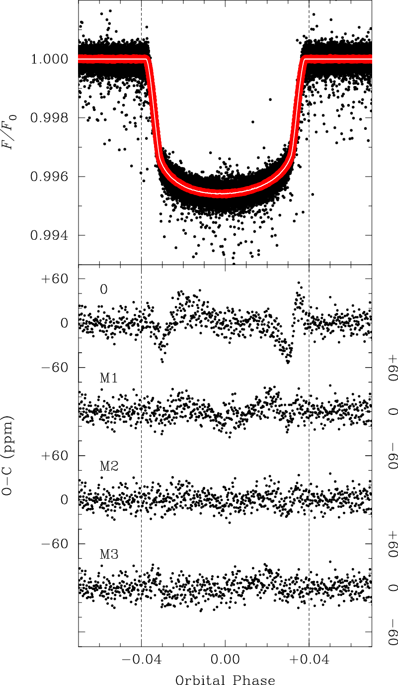 Figure 1
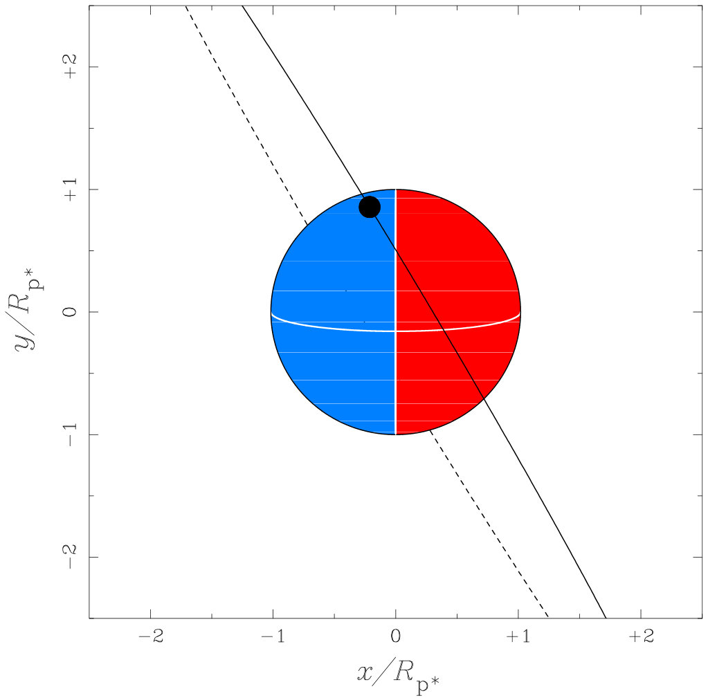 Figure 2
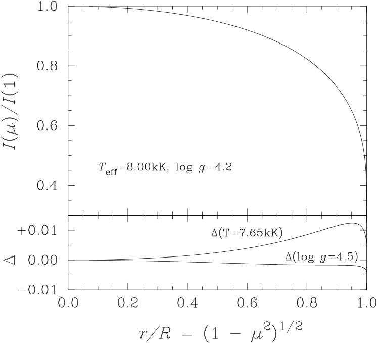 Figure 3
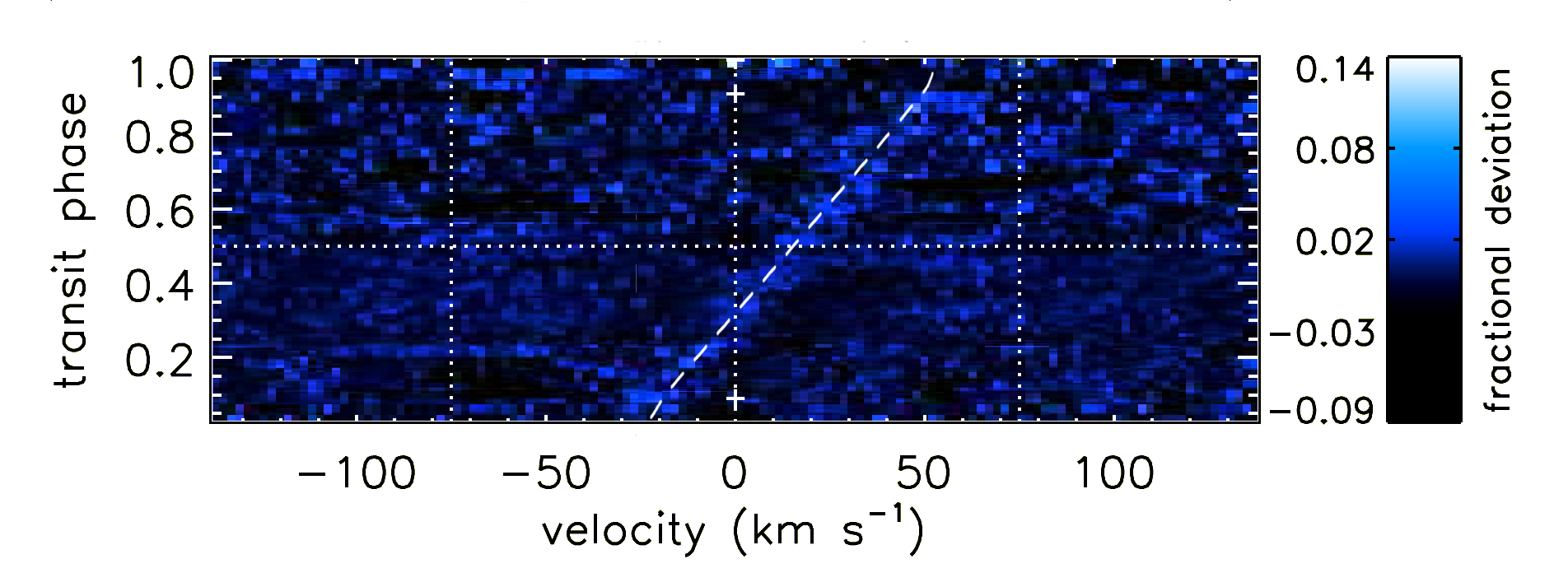 Figure 6
| Parameter | Best-fit value | ||||||
| Model: | M1 | M2 | M3 | ||||
| Stellar: | |||||||
| Effective-temperature parameter∗ (K) | 8084 | 186 | 7987 | 8046 | |||
| Polar-gravity parameter∗ (dex cgs) | 4.27 | 4.32 | |||||
|
Angular rotation rate
(in units of the critical rate) |
0.341 | 15 | 0.343 | 0.320 | |||
| Inclination of stellar rotation axis to line of sight (0–90∘) | 81.137 | 16 | 81.135 | 81.134 | |||
|
Polar radius
(in units of the orbital semi-major axis) |
0.2219 | 4 | 0.2217 | 0.2219 | |||
| ‘Third light’ | 0.451 | 39 | 0.451 | 0.451 | |||
| g.d. | Gravity darkening: ELR | ||||||
| Planetary: | |||||||
| Planetary radius (in units of the orbital semi-major axis) | 0.0190 | 7 | 0.0190 | 0.0190 | |||
| Orbital: | |||||||
| Inclination of orbital angular-momentum vector to line of sight (0–180∘) | 93.319 | 22 | 93.316 | 93.316 | |||
| Angle between the projections onto the plane of the sky of the orbital and stellar-rotational angular-momentum vectors, measured counter-clockwise from the former (0–360∘) | 59.19 | 5 | 59.20 | 59.20 | |||
| Imposed: | |||||||
| Orbital period (d) | 1.76358799 | ||||||
| Projected equatorial rotation speed† () | |||||||
| Rotation period (d) | 1.0596 | ||||||
| Derived stellar parameters: | |||||||
| True polar gravity (dex cgs) | 4.209 | 19 | 4.21 | 4.24 | |||
| / | Polar radius | 1.49 | 7 | 1.48 | 1.61 | ||
| / | Equatorial radius | 1.52 | 7 | 1.51 | 1.63 | ||
| Oblateness | 0.0178 | 17 | 0.0181 | 0.0156 | |||
| / | Relative polar temperature | 1.0118 | 11 | 1.0119 | 1.0103 | ||
| / | Relative equatorial temperature | 0.9939 | 6 | 0.9938 | 0.9947 | ||
| System mass‡ | 1.31 | 17 | 1.29 | 1.64 | |||
| (dex solar) | 0.94 | 3 | 0.92 | 1.00 | |||
| Mean density (g cm-3) | 0.5373 | 11 | 0.5380 | 0.5397 | |||
| Equatorial rotation speed () | 77.3 | 4 | 77.5 | 78.0 | |||
| Rotation period (d) | 0.994 | 23 | 0.987 | ||||
| Other derived parameters: | |||||||
| Planetary radius | 1.28 | 5 | 1.28 | 1.38 | |||
| Angle between orbital and stellar-rotational angular-momentum vectors (0–180∘) | 60.24 | 5 | 60.25 | 60.25 | |||
| Impact parameter () | 0.2609 | 12 | 0.2609 | 0.2607 | |||
| Additional model parameters include , the orbital eccentricity ( assumed here) and longitude of periastron (0–360∘; undefined when ). Best-fit (minimum-) parameter sets are listed; median values of MCMC runs are extremely close to these values. | |||||||
| ∗Used only to evaluate model-atmosphere intensities, and constrained in the present study only by limb darkening; cf. 5.1 †Derived radii scale linearly with , and the mass as ; Appendix A. ‡Mass ratio (Shporer et al. 2014; Esteves et al. 2015; Faigler & Mazeh 2015). | |||||||
Peer Reviews
No public reviews on file for this paper yet. If you reviewed it on a platform where reviews are public (OpenReview, ICLR, NeurIPS, ICML), you can paste yours below so the community can read it here.
Videos
No videos yet. Explain this paper in a talk, walkthrough, or lecture? Add one.
Rapid rotators revisited: absolute dimensions of KOI-13
Ian D. Howarth and Giuseppe Morello
Dept. of Physics and Astronomy, University College London, Gower Street, London WC1E 6BT, UK E-mail: [email protected]
(Accepted 2017 May 17. Received 2017 May 14; in original form 2017 April 19)
Abstract
We analyse Kepler light-curves of the exoplanet KOI-13b transiting its moderately rapidly rotating (gravity-darkened) parent star. A physical model, with minimal ad hoc free parameters, reproduces the time-averaged light-curve at the 10 parts per million level. We demonstrate that this Roche-model solution allows the absolute dimensions of the system to be determined from the star’s projected equatorial rotation speed, , without any additional assumptions; we find a planetary radius , stellar polar radius , combined mass , and distance pc, where the errors are dominated by uncertainties in relative flux contribution of the visual-binary companion KOI-13B. The implied stellar rotation period is within 5% of the non-orbital, 25.43-hr signal found in the Kepler photometry. We show that the model accurately reproduces independent tomographic observations, and yields an offset between orbital and stellar-rotation angular-momentum vectors of .
keywords:
stars: individual (KOI-13) – stars: rotation – stars: fundamental parameters
1 Introduction
One of the many unexpected results to emerge from studies of exoplanets this century has been the discovery of orbits that are not even approximately coplanar with the stellar equator (cf., e.g., Winn & Fabrycky 2015).
The tool traditionally most commonly used to investigate the relative orientations of orbital and stellar-rotation angular-momentum vectors is the Rossiter–McLaughlin (R–M) effect (Holt 1893; Schlesinger 1910111An example of Stigler’s law (Merton, 1957; Stigler, 1980).) – the apparent displacement of rotationally broadened stellar line profiles arising from a body occulting part of the stellar disk. Long established in eclipsing-binary studies (e.g., Rossiter, 1924; McLaughlin, 1924), the R–M effect took on new significance following its detection in the archetypal transiting exoplanetary system HD 209458 (Queloz et al., 2000). The discovery of misaligned planetary orbits in other systems followed (Hébrard et al., 2008; Winn et al., 2009), and sample sizes are now large enough222120 at the time of writing; e.g.,
http://www.astro.keele.ac.uk/jkt/tepcat/rossiter.html to suggest that stars with thick convective envelopes generally have planets with small orbital misalignments, while a broader spread of values is found in hotter stars (Winn et al., 2010; Schlaufman, 2010; Albrecht et al., 2012; Mazeh et al., 2015).
The R–M effect is an essentially spectroscopic phenomenon, being studied through radial-velocity measurements. In principle there is a corresponding photometric signature, arising through Doppler boosting (e.g., Groot 2012), but the signal is too small for any reliable detections to date. Transit photometry does, however, offer potential diagnostics of spin-orbit alignment if the surface-brightness distribution over the occulted parts of the stellar disk is not circularly symmetric. In particular, if the stellar rotation is sufficiently rapid, it can introduce both an equatorial extension and, through gravity darkening, a characteristic latitude-dependent surface-intensity distribution; these effects are capable of defining the relative direction of the stellar rotation axis, and hence of diagnosing misaligned transits (e.g., Barnes 2009).
The first system to be recognized as having a misaligned orbit from photometry alone, without supporting evidence from the R–M effect, was KOI-13 (Szabó et al., 2011; Barnes et al., 2011). Other systems in which asymmetry in the transit light-curve has been interpreted as arising through rotationally-induced gravity darkening include KOI-89 (Ahlers et al., 2015) and HAT-P-7 (KOI-2; Masuda 2015), while the same approach has been used to argue for good alignment of orbital and rotational angular-momentum vectors for KOI-2138 (Barnes et al., 2015). In other cases, modelling of lower-quality data has led to less compelling claims; e.g., PTFO 8-8695 (cp. Barnes et al. 2013; Howarth 2016) and CoRot-29 (cp. Cabrera et al. 2015; Pallé et al. 2016).
In the present paper we re-examine Kepler photometry of transits of KOI-13, using a more complete physical model than previous studies. Our intention is to stress-test the model against data of remarkable quality, and to demonstrate its power to establish absolute numerical values for key stellar and planetary parameters. Following a selective review of the literature on KOI-13 (2), we summarize the model (3) and the data preparation (4). Results are presented and discussed in 5, 6. Appendix A demonstrates how to put the modelling on an absolute scale, given the star’s projected equatorial rotation speed.
2 The KOI-13 system
Kepler Object of Interest no. 13 (KOI-13; historically catalogued as BD +46∘ 2629) was identified as the host of a transiting exoplanet by Borucki et al. (2011). Aitken (1904) had previously noted BD +46∘ 2629 as visual binary with components of comparable brightness, separated by 11 (Howell et al., 2011; Law et al., 2014), which Szabó et al. (2011) showed share a common proper motion. The latter authors identified the marginally brighter component as the transiting system, a result confirmed by Santerne et al. (2012), who found the fainter component, KOI-13B, to be itself a spectroscopic binary.
The basic transit light-curve was modelled by Barnes et al. (2011), who showed that its small asymmetry arises from stellar gravity darkening coupled to spin–orbit misalignment. Subsequent tomography yielded results inconsistent with the obliquity inferred in this first analysis (Johnson et al., 2014), but by imposing the constraint afforded by the spectroscopy, Masuda (2015) was able to identify a geometry that reconciled the spectroscopic and light-curve solutions.
The exquisite quality of the Kepler data has inspired a number of ancillary studies. In particular, the system clearly shows out-of-transit orbital variations arising from Doppler beaming, ellipsoidal distortion, and reflection effects (‘beer’ effects; Shporer et al. 2011; Mislis & Hodgkin 2012; Mazeh et al. 2012). A further, 25.43-hr, periodic signal has been identified in the photometry, and has been suggested as arising either from tidally induced pulsation (Shporer et al., 2011; Mazeh et al., 2012) or from rotational modulation (Szabó et al., 2012).
3 Modelling
The Barnes et al. (2011) and Masuda (2015) analyses of the transit light-curve were both based on a simple oblate-spheroid stellar geometry, and utilised black-body fluxes coupled to a global two-parameter limb-darkening ‘law’. These are reasonable approximations for initial investigations, especially since KOI-13’s rotation is substantially subcritical (cf. Table 1), but we undertook our work in the hope that a somewhat more physically-based model would better constrain the system with fewer ad hoc adjustments.
The basic model is as described by Howarth (2016; Howarth & Smith 2001). Appropriate values for model parameters, and their probability distributions, are determined through Markov-chain Monte-Carlo (MCMC) sampling, with uniform priors unless stated otherwise.
3.1 Star
The star’s rotationally distorted surface is approximated as a Roche equipotential.333Mass distributions from polytropic models give negligibly different results (Plavec, 1958; Martin, 1970). By default, surface angular velocity is assumed to be independent of latitude. Latitude-dependent values of surface gravity, , and local effective temperature, , are calculated self-consistently, taking into account gravity darkening. The stellar flux is then computed as a numerical integration of emitted intensities over visible surface elements.
3.1.1 Intensities
Specific intensities (radiances), , are interpolated from a grid of line-blanketed, solar-abundance LTE models (Howarth, 2011a), integrated over the Kepler passband. The interpolation in angle (, where is the angle between the surface normal and the line of sight) is performed using an analytical 4-parameter characterization
[TABLE]
(Claret, 2000), which reproduces individual numerical values to 0.1% (Howarth, 2011a).
3.1.2 Modelled effective temperature, gravity
Surface distributions of temperature and gravity are needed in order to evaluate model-atmosphere emergent intensities (and for no other reason). These parameters are completely specified by the adopted gravity-darkening law (3.1.3), plus any suitable normalizations; we use the base-10 logarithm of the polar gravity in c.g.s. units, , and the stellar effective temperature,
[TABLE]
(where is the Stefan–Boltzmann constant and the integrations are over surface area).
While the use of model-atmosphere intensities removes the need for ad hoc limb-darkening parameters, this is at the expense of assumptions that, first, the effective temperature and polar gravity are known with adequate precision to give a sufficiently faithful representation of limb darkening, and secondly, that the model-atmosphere calculations predict the emergent intensities reliably. Anticipating that neither assumption need necessarily be valid (e.g., Howarth 2011b), we draw an explicit distinction between the actual physical quantities , and their model-parameter counterparts , (where the superscript is intended to indicate a ‘light-curve’, or ‘limb-darkening’, determination; cf. 5).
3.1.3 Gravity darkening
It is not immediately obvious whether gravity darkening in KOI-13 should be modelled according to a recipe appropriate for radiative or convective envelopes. While the literature documents a surprising large dispersion for estimates of its effective temperature (7650–9107 K; Shporer et al. 2014, Szabó et al. 2011, Brown et al. 2011, Huber et al. 2014, with claimed precisions that are considerably smaller than the spread of results), the more detailed studies tend towards values at the lower end of the range. This puts not very far from the boundary between convective and radiative regimes, around K (e.g., Claret 1998). Because of this, we ran several sequences of models using a generic gravity-darkening law,
[TABLE]
with the gravity-darkening exponent as a free parameter. These models all migrated to solutions with exponents very close to the von Zeipel (1924) value of , as was also found by Masuda (2015).
For most model runs, we actually used the parameter-free gravity-darkening model proposed by Espinosa Lara & Rieutord (2011), which is close to von Zeipel gravity darkening at the subcritical rotation appropriate to KOI-13. This ‘ELR’ formulation has a somewhat firmer physical foundation than the original von Zeipel analysis, and gives better agreement with, in particular, optical interferometry of rapid rotators (e.g., Domiciano de Souza et al. 2014).
3.2 Transit
Transits are modelled by assuming a completely dark occulting body of circular cross-section, in a misaligned circular orbit; although an orbital eccentricity has been inferred from out-of-transit photometry of KOI-13 by Esteves et al. (2015), this has negligible consequences for our study. The contamination of the transit light-curve by KOI-13B (spatially unresolved in the Kepler beam) is characterized by its fractional contribution to the total signal, or ‘third light’ () in the nomenclature of traditional eclipsing-binary studies.444Of course, the exoplanetary ‘second light’ is extremely small.
3.3 Parameters
Table 1 lists one set of basic parameters that fully specify the model (other combinations are possible). We stress that the geometry of the model is fundamentally scale-free; all linear dimensions are expressed in units of the orbital semi-major axis, while times are implicitly in units of the orbital period. The extent of effects arising from rotational distortion is determined by , the ratio of the rotational angular velocity to the critical value at which the effective equatorial gravity is zero; a value for the stellar mass, often assumed in similar studies, is not required.
4 Data preparation
We used the full set of short-cadence Pre-search Data Conditioning Simple Aperture Photometry (PDCSAP) data, which are publicly available through the Kepler Input Catalog (KIC; Brown et al., 2011). The PDCSAP results are produced by the standard Kepler pipeline, which removes instrumental artifacts, and span 2009 June to 2013 May.
The sampling step of 58.9 s corresponds to of the 1.7-d orbital period. The maximum difference between ‘instantaneous’ and exposure-integrated model fluxes in the parameter space of interest is 6 parts per million (ppm), which is small enough to be neglected (deviations exceed 1 ppm for a phase range of ¡0.001).
The system shows out-of-transit orbital variations arising from beer effects (2). Even over the limited phase range that we model, \pm{0.1}$$P_{\rm orb} around conjunction, the amplitude of these effects is 40 ppm, which is far from negligible. We treated these effects as a perturbation on the basic model, and corrected for them by using the empirical three-harmonics model555The model defined by eqtn. (11) and Table 5 of Shporer et al. has to be reversed in both and . described by Shporer et al. (2014).
The 25.43-hr signal has a semi-amplitude variously reported as 12–30 ppm (Shporer et al. 2011; Mazeh et al. 2012; Szabó et al. 2012); in the limited out-of-transit phase range of our data we find a semi-amplitude of only 6 ppm, suggesting that the amplitude may be variable. Although the period is close to a 3:5 resonance with the orbital period (Shporer et al., 2011), the ratio is not exact. Consequently this signal is ‘mixed out’ over the 4-year span of the observations when phased on transits, and effectively becomes only a minor source of additional stochastic noise.
In order to reduce the 299 423 individual observations down to a manageable subset for MCMC modelling, for each of 577 separate transits the data were first phased (according to the ephemeris used in the current MCMC cycle); corrected for beer effects; and rescaled to give a median out-of-transit flux of one.666‘Out of transit’ was taken as , where orbital phase is measured in the range about conjunction. In principle, any free parameters in the adopted functional form for the ephemeris could be allowed to ‘float’ in the fitting process; in practice, we adopted a linear ephemeris with a fixed period ( d; Shporer et al. 2014), but allowed the time of conjunction to vary.
We then compressed the resulting data by taking median normalized fluxes in phase bins of 0.0002 (about half the integration time of individual observations), whence each bin contained 300 data points. The maximum change in normalized flux between the central times of bins is , which is comparable to the dispersion of the individual data points ( out of transit), but large compared to the precision of the binned data (); consequently, we tagged the median flux in each bin with the mean time of all observations in that bin (invariably close to the mid-bin time) rather than its original, individual phase.
5 Fit Results
As a basis for subsequent discussion, we first present the results of an initial ‘maximally constrained’ model, in which only (effectively) geometric parameters were adjusted. ELR gravity darkening (Espinosa Lara & Rieutord, 2011) and model-atmosphere limb-darkening were used, along with fixed values for (7650 K; Shporer et al. 2014) and (0.45; Szabó et al. 2011). The results of this ‘model 0’ are illustrated in Fig. 1, and show relatively large residuals during ingress and egress (50 ppm).
We investigated the origin of these residuals through extensive exploration of model parameters. Adopting eqtn. (2) with free essentially reproduced von Zeipel’s law, which in turn gives sensibly identical results to the ELR model (unsurprisingly, since the latter is known to reproduce von Zeipel at low to moderate rotation). Moderate adjustments to had similarly small consequences for the quality of the model fits. These experiments identified errors in the limb darkening as the principal cause of the discrepancies.
We addressed this issue in three ways. First, we replaced the near-exact represention of the angular dependence of the model-atmosphere intensities afforded by eqtn. (1) with a simple quadratic limb-darkening law,
[TABLE]
with the coefficients , as free parameters. In applying this law globally (in common with, e.g., Masuda 2015), we abandon any latitudinal temperature dependence of the coefficients.
Secondly, in a gesture towards retaining temperature-dependent limb-darkening while introducing only a single additional free parameter, we investigated scaling the linear () term in the 4-coefficient characterization.777There is a minor inconsistency in both the first and second approaches, in that the integral of intensity over angle will, in general, no longer exactly match the model-atmosphere flux, but this is unimportant for our application.
Thirdly, recognizing that there is a temperature dependence of the model limb darkening, we allowed the effective-temperature parameter to float; that is, we characterize the model-atmosphere intensities by rather than (3.1.2).
Unsurprisingly, all three approaches gave improved model fits, but it is noteworthy that quite small adjustments to the model effective temperature have significant consequences at the 10 ppm level of precision, solely through the modest sensitivity of to this parameter. In practice, allowing to float also led to smaller residuals than the other approaches in our numerical experiments; we adopt the corresponding results for this reason, and to avoid introducing additional ad hoc parameters. Numerical values for this ‘model M1’ are included in Table 1, and it is confronted with the observations in Fig. 1. Fig. 3 is a simple cartoon illustrating the implied geometry of the system.
Model-atmosphere intensities are a function of not only temperature, but also surface gravity (as well as abundances and microturbulence). The true polar gravity, (which, with , characterizes the overall surface-gravity distribution) is not a free parameter in our model (6). However, we can allow the value used in obtaining the model-atmosphere intensities, , to ‘float’ as, effectively, an additional limb-darkening parameter. Doing this naturally affords further, albeit slight, improvement in the model fit (model M2 in Table 1 and Fig. 1).
The remaining systematic residuals (peaking at 10 ppm) may arise from orbital evolution over the duration of the Kepler observations (Szabó et al., 2012; Szabó et al., 2014; Masuda, 2015), since the time-averaged light-curve will not correspond to any single-epoch photometry. Modelling the time-dependent behaviour is beyond the scope of the current paper, partly because of the substantial computing requirements required to model necessarily less compacted datasets (we may return to this in future work), but also because our discussion of third light (5.2) emphasizes that the uncertainties on fundamental parameters (our main interest here) are likely to be dominated by other factors.
5.1 Effective temperature and limb darkening
We recall that the effective-temperature ‘determination’ in the model is not a traditional, direct measurement of the actual stellar effective temperature, ; rather, is simply a parameter which optimises model-atmosphere limb darkening (over the range of surface temperatures) to give a best match to the transit data.888The same caveat applies to ; the actual value of is fixed by other model parameters; (6). Only if the calculated model-atmosphere intensies are sufficiently accurate will correspond to the actual effective temperature.
However, it is noteworthy that, in practice, the optimised value of falls well within the range of direct determinations; while adopting only a moderately different fixed value gives relatively large residuals. This highlights the importance of establishing the correct value of when comparing empirical and theoretical limb-darkening coefficients (or when adopting the latter). Figure 2 shows the limb darkening for a model atmosphere at kK, , representative of the parameter space within which our solutions fall. The maximum difference in normalized intensity, , between this model and one at 7.65 kK is less than 2%, and yet this difference accounts for almost all of the residuals for Model 0 shown in Fig. 1.
5.2 Third light
The third light of the unresolved optical companion KOI-13B is (literally) a nuisance parameter in our modelling. For our MCMC runs we experimented with initial values of –0.49 (–0.04), which bracket most observational determinations in the literature999Howell et al. (2011) report notably discordant values of –1.1 at 600–700 nm. Although the literature values are for diverse wavebands, the KOI-13A and B components are of similar spectral types and colours (Szabó et al., 2011), so any wavelength dependence of should be small in the optical regime. (Fabricius et al., 2002; Adams et al., 2012; Law et al., 2014; Shporer et al., 2014), at steps of 0.02.
We found that the adopted third light always clung very close to the initial estimate in our MCMC modelling, rather than converging onto a value representing the global minimum in hyperspace. This contrasts with the behaviour of other parameters, whose values freely migrated over relatively large ranges during ‘burn-in’. Adjusting the proposal distribution did not alleviate this issue.
We believe that this outcome may arise because the transit light-curve contains almost no information on the extent of third-light dilution (cf., e.g., Fig. 8 of Seager & Mallén-Ornelas 2003). Although we might anticipate that this should be reflected in a wide distribution in acceptable values, rather than a narrow one, in practice the set of other parameters essentially locks in , which can therefore be regarded, in a limited sense, as a ‘derived’ parameter, given the system geometry, rather than a free one.
The inferred numerical values for other parameters therefore depend somewhat on , to a degree that typically exceeds the formal errors on any given model. For example, smaller means a shallower true transit depth, and hence implies smaller (). In recognition of this, while we adopt solutions with input (which yield the smallest residuals), we give errors in Table 1 which are the quadratic sum of the 95%-percentile ranges on those models and the maximum differences with the ‘best-fit’ parameters from models with –0.49 (where the latter term dominates).
5.3 Rotation period
Our initial solutions (e.g., models M1 and M2) yielded rotation periods close to 24 hr, only 5% from the 25.43-hr period found in the Kepler photometry (Shporer et al., 2011; Mazeh et al., 2012; Szabó et al., 2012). Although rotational modulation had not been widely anticipated for stars hotter than the ‘granulation boundary’ marking the transition from radiative to convective envelopes (e.g., Gray & Nagel 1989), evidence is beginning to accumulate for starspots, of some nature, in A-type stars (Balona, 2011, 2017; Böhm et al., 2015), encouraging consideration of the possibility that we are seeing a rotational signature in KOI-13 ( kK corresponds to spectral type A5–A7), as suggested by Szabó et al. (2012).
We can impose the constraint of fixed on the model, which links to in the MCMC chains (Appendix A, eqtn. 5). The results of this model M3 are reported in Table 1; the fit quality is quite reasonable (Fig. 1). Because the transit depth essentially fixes , the main effect of imposing a longer rotation period is to decrease the angular rotation rate, which for given leads to a larger stellar radius, and hence, for fixed density, a higher stellar mass, as discussed in the Section 6.
5.4 Tomography
There are no published Rossiter–McLaughlin investigations of KOI-13, but Johnson et al. (2014) conducted a detailed tomographic study, providing a velocity-resolved map of the transit.
Our model allows stellar velocities (R–M effect or tomographic counterpart) to be evaluated directly. This can be accomplished by synthesizing the spectrum as a function of orbital phase, and subjecting the ensemble of synthetic spectra to the same analysis as the observations (e.g., cross-correlation, or tomography). However, for the present study we simply take the intensity-weighted average radial velocity,
[TABLE]
where the integration is over area, and the (weak) wavelength dependence of the model velocity comes about because of the wavelength dependence of intensities on limb darkening and temperature. To evaluate the R–M effect the integration is conducted over all visible elements, while taking the velocity of all occulted elements models the tomographic signature.
The predicted locus of velocity vs. phase from the light-curve solution is compared to the Johnson et al. map in Fig. 4. The agreement is very satisfactory, arising from the accord between the values of projected obliquity and impact parameter obtained from the independent tomographic and photometric solutions (, ).
6 System parameters
Any fundamentally geometric transit model, such as employed here, is of necessity scale free. Consider Fig. 3; there is no indication of whether this is a small, nearby system, or a large, distant one.
Nevertheless, for given orbital period, a large, distant system must have greater orbital velocities, and hence greater masses, than a smaller, nearby system. This relationship between scale and mass is codified in Kepler’s third law, which leads directly to a constraint on , and hence, given the dimensionless radius , to the stellar density (e.g., Seager & Mallén-Ornelas 2003) – but not the mass and radius separately.
Barnes et al. (2011) suggested that rotational effects, and specifically gravity darkening, can, in principle, lift the “density degeneracy”, through the dependence of on mean stellar radius . However, in the Roche approximation the light-curve depends on rotational effects only through the ratio ; to get to requires calculation of , which itself has an dependence. Consequently, is actually scale-free (as shown analytically in Appendix A), and a Roche-model analysis of the transit light-curve alone cannot break the mass/radius degeneracy in .
Of course, if the orbital velocities can be established for both components, these determine the absolute scale – the standard ‘double-lined eclipsing binary’ approach. However, an alternative, independent means of establishing the orbital semimajor axis (and hence other system parameters) is available if , the stellar rotation period, , the axial inclination, and , the line-of-sight component of the equatorial rotation speed, can be determined; these immediately yield the equatorial radius,
[TABLE]
The quantities and can be estimated if the circular symmetry of the projected stellar disk is broken. A familiar example is when starspots are present, but gravity-darkened stars have the same potential (since relates, indirectly, to ). Introducing the observed projected equatorial rotation speed, , as a constraint on the light-curve solution therefore affords usefully tight limits on the absolute dimensions of the system. The straightforward algebra is set out in Appendix A.
There are two precise determinations of projected rotation speed of KOI-13A in the literature, in good mutual agreement: and (Johnson et al., 2014; Santerne et al., 2012). We adopt the latter, more precise value in order to calculate the system dimensions reported in Table 1.
[Our referee raised the point that the precision of these results may not reflect their accuracy, an observation with which we fully concur (cf., e.g., Howarth 2004). However, as shown in Appendix A (eqtn. 5), the semi-major axis scales linearly with ; radii converted from normalized to absolute values scale in the same way, while the absolute system mass scales as , from Kepler’s third law. Hence the results, or uncertainties, are readily reassessed if another value for the projected equatorial rotation speed is preferred.]
6.1 Distance
The effective temperature determines the surface brightness; given the size of the star the absolute magnitude follows, and hence the distance. We find
[TABLE]
where the second term is an empirical fit to models with ; model-atmosphere Johnson -band fluxes are from Howarth (2011a); and we neglect the further, unimportant, dependences of on and .
There is a surprisingly large dispersion in the photometry of KOI-13 catalogued in the Vizier system of the Centre de Données astronomiques de Strasbourg, most of which clearly refers to the combined light of the visual binary. We adopt the spatially resolved Tycho-2 photometry, which transforms to for KOI-13A (with an uncertainty of 0.05; Høg et al. 2000). Foreground reddening is estimated as from Green et al. (2015), whence
[TABLE]
i.e., pc, with an uncertainty of perhaps 25 pc.
7 Conclusions
We have conducted a new solution of Kepler photometry of transits of KOI-13b, obtaining results that are substantially in agreement with those found by Masuda (2015), and in accord with the tomography reported by Johnson et al. (2014). The solution yields both the projected and true angular separations of the orbital and stellar-rotation angular-momentum vectors. We emphasize that any photometric solution is necessarily scale-free (e.g., does not require a stellar mass to be assumed); but demonstrate that, by adopting a value for , the absolute system dimensions and mass can be established. Allowing for the full range of solutions (Table 1; third light –0.49, free or fixed stellar rotation period), we obtain a planetary radius , stellar polar radius , and a combined mass . All solutions place KOI-13 in an unremarkable location in the main-sequence mass–radius plane (e.g., Eker et al. 2015).
Appendix A Scaling
The photometric solution establishes reasonably precise values for , , and ; and we have the ancillary observational quantities and to good accuracy.
In the Roche model, the critical angular rotation rate at which the equatorial surface gravity is zero is
[TABLE]
The equatorial rotation speed is
[TABLE]
where, again in the Roche model, the function is given by
[TABLE]
(Harrington & Collins, 1968). Using Kepler’s third law,
[TABLE]
for the mass in eqtn. (4), and rearranging, gives the semi-major axis:
[TABLE]
All terms on the right-hand side are ‘known’, except the mass ratio , which it may often be reasonable to assume to be negligibly small if no numerical estimate is available. Having evaluated the orbital semi-major axis, the linear dimensions of the system components, and the mass, follow (radii from , and from Kepler’s third law).
Using similar reasoning as above, we also have
[TABLE]
Thus in the Roche model the rotation period (or, equivalently, ) is scale free, and of itself offers no independent leverage on absolute values of or . However, if is known from independent considerations, it may be used to constrain the combination (5.3).
The reference list from the paper itself. Each links out to its DOI / PubMed record.
- 1Adams et al. (2012) Adams E. R., Ciardi D. R., Dupree A. K., Gautier III T. N., Kulesa C., Mc Carthy D., 2012, AJ , 144, 42 · doi ↗
- 2Ahlers et al. (2015) Ahlers J. P., Barnes J. W., Barnes R., 2015, Ap J , 814, 67 · doi ↗
- 3Aitken (1904) Aitken R. G., 1904, Lick Observatory Bulletin , 3, 6 · doi ↗
- 4Albrecht et al. (2012) Albrecht S., et al., 2012, Ap J , 757, 18 · doi ↗
- 5Balona (2011) Balona L. A., 2011, MNRAS , 415, 1691 · doi ↗
- 6Balona (2017) Balona L. A., 2017, MNRAS , 467, 1830 · doi ↗
- 7Barnes (2009) Barnes J. W., 2009, Ap J , 705, 683 · doi ↗
- 8Barnes et al. (2011) Barnes J. W., Linscott E., Shporer A., 2011, Ap JS , 197, 10 · doi ↗