Contract Design for Energy Demand Response
Reshef Meir, Hongyao Ma, Valentin Robu

TL;DR
This paper introduces DR-VCG, a novel demand response mechanism using VCG pricing that improves participation, reliability, and cost-efficiency in energy demand management.
Contribution
The paper presents DR-VCG, a flexible, truthful, and computationally efficient demand response mechanism that outperforms existing contracts in participation and reliability.
Findings
DR-VCG achieves higher consumer participation.
It increases reliability of demand reduction.
It significantly reduces total costs compared to current mechanisms.
Abstract
Power companies such as Southern California Edison (SCE) uses Demand Response (DR) contracts to incentivize consumers to reduce their power consumption during periods when demand forecast exceeds supply. Current mechanisms in use offer contracts to consumers independent of one another, do not take into consideration consumers' heterogeneity in consumption profile or reliability, and fail to achieve high participation. We introduce DR-VCG, a new DR mechanism that offers a flexible set of contracts (which may include the standard SCE contracts) and uses VCG pricing. We prove that DR-VCG elicits truthful bids, incentivizes honest preparation efforts, enables efficient computation of allocation and prices. With simple fixed-penalty contracts, the optimization goal of the mechanism is an upper bound on probability that the reduction target is missed. Extensive simulations show that…
Click any figure to enlarge with its caption.
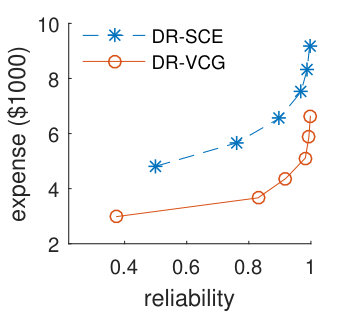 Figure 1
 Figure 1
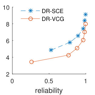 Figure 1
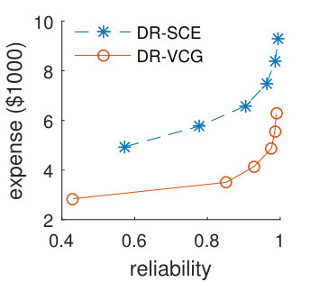 Figure 2
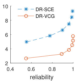 Figure 2
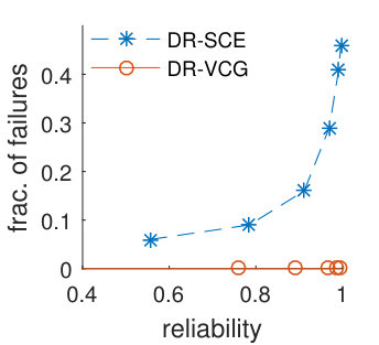 Figure 3
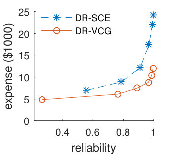 Figure 3
Peer Reviews
No public reviews on file for this paper yet. If you reviewed it on a platform where reviews are public (OpenReview, ICLR, NeurIPS, ICML), you can paste yours below so the community can read it here.
Videos
No videos yet. Explain this paper in a talk, walkthrough, or lecture? Add one.
Contract Design for Energy Demand Response
Reshef Meir
Technion – Israel Institute of Technology
Haifa, Israel
&Hongyao Ma
Harvard University
Cambridge, MA, US
&Valentin Robu
Heriot-Watt University
Edinburgh, UK
Abstract
Power companies such as Southern California Edison (SCE) uses Demand Response (DR) contracts to incentivize consumers to reduce their power consumption during periods when demand forecast exceeds supply. Current mechanisms in use offer contracts to consumers independent of one another, do not take into consideration consumers’ heterogeneity in consumption profile or reliability, and fail to achieve high participation.
We introduce DR-VCG, a new DR mechanism that offers a flexible set of contracts (which may include the standard SCE contracts) and uses VCG pricing. We prove that DR-VCG elicits truthful bids, incentivizes honest preparation efforts, enables efficient computation of allocation and prices. With simple fixed-penalty contracts, the optimization goal of the mechanism is an upper bound on probability that the reduction target is missed. Extensive simulations show that compared to the current mechanism deployed in by SCE, the DR-VCG mechanism achieves higher participation, increased reliability, and significantly reduced total expenses.
1 Introduction
Power system operation involves many challenges, driven by the requirement that supply equals demand at all times. Too much supply may lead to overload on the grid, whereas excessive demand may lead to shortages and blackouts. The problem is aggravated by the fact that consumption tends to vary sharply due to certain events (for example, surges in consumption during heatwaves), whereas increasing the supply is typically slow and costly. Even if the power company wants to shift some of the demand to a different time, it cannot coerce the consumers to do so, and may only affect their behavior by using monetary incentives, such as increasing electricity price during peak-demand times. As in other markets, consumers may respond to incentives in different ways based on their own preferences. Unlike some other markets, the serious consequences of failure to meet demand, and the large uncertainty about how consumers may react to incentives, requires the power company to guarantee there is enough slack on the supply side.
The DR-SCE mechanism
Demand Response (DR) programs are used by power companies to handle surges in demand by reducing consumption rather than increasing production. Typically, when a surge is predicted one day ahead of time, the company lets consumers bid on how much consumption they can reduce. Each consumer is being paid a fixed \0.5$ per reduced kWh, but only if the reduced consumption is between 50% and 150% of her bid. We call this system the DR-SCE mechanism, as it is used by Southern California Edison (c.f. Patterson et al. (2014)) (as well as other companies such as PG&E Hansen et al. (2014)).
DR-SCE has several shortcomings: incentives for participation are often insufficient (only 12% of registered participants in 2012-2013 submitted any bids), the system does not capture the very different consumption profiles of consumers, and does not filter out unreliable bidders. Yet, being a widely deployed DR system, we treat DR-SCE both as a starting point and as a benchmark for new mechanisms.
Contribution
We propose a novel DR-VCG mechanism for selecting and incentivizing a subset of consumers to reduce consumption. The grid offers a set of contracts defined by some desired reduction target and a penalty scheme, and agents may bid how much they want to get paid on for accepting each contract. The mechanism then selects a subset of contracts that minimizes the sum of bids, and applies VCG prices to pay the agents. As a result, it is a dominant strategy for all agents to bid their true costs.
We show that for natural penalty schemes, the sum of bids is a good proxy for the reliability of the joint contract, as high bids are indicative of low individual reliability. We show that the current contracts used by SCE and PG&E can still be offered under DR-VCG (to allow for easy transition and backward-compatibility). We demonstrate via examples and simulations that even when restricted to offering SCE-like contracts, DR-VCG dominates DR-SCE in terms of reliability and grid expense.
This is the full version of a paper accepted to IJCAI-2017 Meir et al. (2017). All omitted proofs are available on Appendix B.
Related Work
A number of recent works have discussed how groups of agents can be coordinated and incentivized to shift power demand Haring et al. (2016); Zhang et al. (2015); Su et al. (2014). Considering strategic agents, Rose et al. (2012) and Akasiadis and Chalkiadakis (2013) propose the use of scoring rules to incentivize truthful reports about expected future generation or consumption. However, scoring rule approaches are not concerned with selection of agents to satisfy a system-wide reliability constraint. Li et al. (2015) consider agents bidding using supply curves, and study the market equilibria for this setting. They do not, however take a mechanism design perspective or try to guarantee truthfulness. Mechanism design approaches for aggregating load apply either variations of VCG Samadi et al. (2012); Chapman and Verbic (2017), or a new “staggered clock-proxy” auction Nekouei et al. (2015). Neither work considers the crucial issue of reliability, i.e. in practice not all agents selected to respond will do so. A different variation of VCG pricing was used by Porter et al. (2008) to align the incentives of agent in face of possible failures in general mechanisms. However their version requires full revelation (which is problematic in practical DR programs), and is aimed at maximizing social welfare rather than reliability.
The work closest to ours is Ma et al. (2016), who propose a mechanism that allows agents to bid on the maximal penalty for failing the DR contract, while Ma et al. (2017) extend this work to include uncertainty about costs. Our work takes a different approach, which generalizes currently used contracts and, in our view, is more geared to practical applications.
2 Model
We consider a single power utility or system operator (henceforth, the grid), and a set of consumers (or agents) who are registered to a demand response program.
The most important task of the grid is to cut down consumption by at least energy units (say, ) during the DR event. Given that this target is met, the grid would like to minimize payments to the agents. The baseline consumption profile of each agent is assumed known from past consumption data, so the grid can measure how much each agent reduced in practice.
2.1 Contracts
A contract in our model is defined by a pair , where is a commitment goal in energy units and is a penalty function, mapping the realized energy reduction to a monetary penalty . A-priori, is unconstrained, and is merely a non-binding declaration of the agent’s intentions. It makes sense to consider more specific classes of penalties that attach the penalty to the commitment goal.
Fixed contracts
A Fixed penalty contract is defined by a pair , and the penalty is set to if and 0 otherwise. In other words, the agent commits to reduce , or otherwise pay a penalty of . See Fig. 1(a).
Cliff contracts
A Cliff penalty contract is defined by a tuple where . It has the following form:
[TABLE]
We can think of a Cliff penalty function as a plateau where the penalty is 0 whenever the commitment is met. Failure to meet the goal results in a linear penalty, where beyond a certain point the penalty becomes a constant, and the utility drops sharply (hence a “cliff”). See Fig. 1(b).
Clearly any Fixed contract is a Cliff contract. As we will later see, the SCE payment scheme can be implemented as a particular Cliff penalty scheme, so even restricting our mechanism to using Cliff contracts is sufficient to generalize the SCE system.
Optimal contract sets
For what follows, we assume no structural restriction on contracts or penalty schemes. We simply assume that a set of contracts are offered, and is the penalty for an agent who signs up for contract and reduces consumption by . Since the value of a contract to an agent is always non-positive, denote by the bid of agent on contract .111The bid is supposed to reflect the various costs involved in taking the contract: preparation cost, online adjustment costs, the expected penalty and so on. We elaborate on this in the next section. Then for a subset of contracts , we denote the sum of bids by .
In addition, the grid may pose a restriction on which sets of contracts are valid: we denote by all valid sets of contracts. In this work, we use this constraint to impose a lower bound on (declared) reduction in consumption, thus
[TABLE]
In other words, includes all sets of contracts that claim to reduce at least units of consumption, and each agent has at most one contract. For an agent , we denote , that is, the sum of bids over all agents in except . We sometimes denote as a selected agent (meaning there is some s.t. ).
An optimal contract set is a set of individual contracts that minimizes the sum of bids, i.e. .
2.2 The DR-VCG Mechanism
We define the DR-VCG mechanism, for assigning demand response contracts using Vickrey-Clarke-Groves (VCG) payments. The grid publishes a finite set of contracts .222The analysis works also for a variant of the mechanism where agents may propose new contracts. See Appendix A. Each agent submits a single bid on each contract . For now, we can think of as some proxy of the cost required from when taking on contract . The mechanism finds the optimal valid set of contracts by solving .
For a set of agents , a set of contracts , and a reduction goal , we can plug in our more specific optimization goal and constraints. We get the optimal subset of contracts as
[TABLE]
We denote , and omit some of the parameters when they are clear from the context. Then, for each selected agent , the individual rewards are computed as the VCG payments with the Clarke pivot rule Clarke (1971). Informally, the sum of bids is analog of the social cost, and the VCG payment is the positive externality the agent’s presence has on the rest of the agents. Formally, for each ,
[TABLE]
The reward is paid to the agent up front, regardless of how much reduction it eventually achieves in practice.
Finally, for each , the selected agent pays to the grid, where each is the realized reduction of agent . The utility of agent depends on the reward, the penalty, and the investment costs required to meet the contract. We analyze agents’ incentives and utilities in the next section.
Example 1** (Running example).**
Suppose we apply the DR-VCG mechanism with a single fixed contract . There are three agents that submit bids of , and the goal for the grid is set to .
The optimal set of contracts that meets is with . The rewards are:
[TABLE]
so in total the grid pays (some of which it might get back as penalties).
3 Analysis
Complexity
In order to run the DR-VCG mechanism, we should be able to efficiently compute the optimal contract set and prices. Suppose that energy units (including the reduction goal ) are integers.
Theorem 1**.**
For any sets of agents and Cliff contracts , both of and (and thus also VCG prices) can be computed in time polynomial in .
In the general case, finding an optimal set of contracts is NP-hard even for fixed contracts, by a reduction from the Knapsack problem Karp (1972) (details omitted).
However, the knapsack problem is solvable by dynamic programming when the units are bounded integers, and a similar algorithm can be applied to our problem (intuitively, compute dynamically the optimal contract sets for agents for ). Hence we get Theorem 1.
3.1 Incentives
To make things concrete we will describe a particular probabilistic model from which we can derive agents’ costs, and will show how under this model the incentives of the agents align nicely with those of the grid. However the claim the agents’ dominant strategy is to reveal their true costs does not depend on this interpretation, and holds whenever agents can attribute a well-defined cost to each contract.
Effort and types
In general, agents do not know with certainty the amount of energy they will be able to reduce, as this depends on some unknown factors such as urgent service orders, last minute clients and so on. Moreover, preparation may have some cost (e.g. due to changing the work schedule, or turning down orders). By investing a higher effort/cost, an agent might be able to commit to saving more energy.
The type of each agent is given by a distribution . In detail, is the probability that by investing , agent will reduce exactly units of consumption (thus for all ).333Investment may include preparation costs, on-line actions required to produce the energy cut , opportunity cost, and so on. We assume agents are always trying to maximize their utility.
A straightforward approach would be to ask agents to report their types (and then apply some version of VCG). However, a language to report an arbitrary distribution may be very complicated. Further, unsophisticated agents like small households may not know their own distribution (or even what is a distribution). Fortunately, our DR-VCG does not require the agents to report any such distribution.
Fix an agent who accepted a contract (with penalty scheme ) and gets paid reward . If she decides to invest , she will pay an expected penalty of , and her expected utility would be:
[TABLE]
Therefore, the optimal investment an utility maximizing agent should make for contract should be
[TABLE]
In words, when agent is signed up for contract , investing will minimize her total cost (investment + penalty). We denote this cost by . We refer to as the cost type of agent , which is derived from her type and .
The total expense (TE) of the mechanism can be computed as the sum of rewards paid to the agents minus expected penalties: (assuming agents invest optimally).
A mechanism is truthful if it is a dominant strategy for any agent to report her true cost on any contract .
A mechanism is individually rational (IR) if for every pair selected by the mechanism, (that is, by participating each agent does not lose in expectation).
Theorem 2**.**
Consider DR-VCG with arbitrary .
For every contract , it is a dominant strategy for agent to bid ; 2. 2.
If contract is selected, it is a dominant strategy for to invest ; 3. 3.
The mechanism is IR.
Proof sketch.
Intuitively, we show that VCG payments are market clearing (following similar proofs in other domains, see Nisan (2007)), i.e. that no agent prefers a different contract (or no contract) under the given prices . Since the prices that agent faces are independent of her bids, it is a dominant strategy to report truthfully. Once contract is selected, then . By definition, this is maximized by investing . ∎
Example 2**.**
Consider three agents, where each one can reduce consumption by kWh without effort. However, agents have different reliability and only manage to hold their commitment with a probability of and , respectively (and otherwise reduce [math]). Suppose that the goal of the grid is kWh.
Consider the DR-VCG mechanism with a single fixed contract . Since agent 1 always meets her commitment, . For the others, (as agent 2 fails w.p. ), and , i.e. are exactly the bids in Ex. 1. The selected set is (the DR-VCG mechanism filters out the least reliable agent). The total expense of the grid is (expected penalty of from agent 2).
3.2 Fallback options and reserve costs
In general, the grid may not find enough agents to meet the reduction goal , and may thus need to use some fallback option like a standby generator or emergency blackouts. For every amount we denote by the cost for the grid of using its fallback option to reduce consumption/increase production by units. E.g. if the total cost of demand response contracts exceeds , then the power company is better off without assigning any contracts, or the fallback options can be used to fill up some gap between and . A fallback option can be simply added to the mechanism as a ‘virtual agent’ that bids on the fixed contract . This is similar to the role of reserve prices in auctions. The reserve costs guarantee that: (I) The grid finds a cheap set of solutions, whether these solutions are contracts with agents or external options; and (II) For any , the reward is bounded: where .
4 Reliability and Expenses
The incentive analysis we presented goes through for any set of contracts. Yet, the goal of the grid is to match demand and supply, preferably at low total expenses, which is a-priori not the same as minimizing the sum of bids. By restricting DR-VCG to use structured constructs we can relate this goal.
We next analyze how the sum of bids relates to reliability, i.e. the probability that the reduction target is met. A detailed example comparing reliability and payments across mechanisms is in Appendix C.
4.1 Fixed penalty contracts
Denote by the probability that a quantity of at least is reduced under contracts . Then is the reliability of the DR-VCG mechanism. We would like to measure or bound , which is the probability that the mechanism fails to meet the lower bound reduction (we may omit some of the parameters).
Proposition 3**.**
Let for some fixed , then . This bound is tight.
Proof.
For any agent that is assigned a contract : The optimal investment is . The expected penalty is
[TABLE]
i.e., proportional to the probability it will undershoot the commitment . The DR-VCG mechanism minimizes
[TABLE]
that is, a combination of the total investment and the sum of individual failure probabilities. Note that
[TABLE]
Thus,
[TABLE]
To see why the bound is tight, observe that the inequalities in the proof are tight if (respectively): (a) failure events are disjoint (i.e. maximally negatively correlated);(b) agents never reduce more than ; (c) the reduction goal is met exactly (); and (d) investments are [math]. ∎
Thus a fixed penalty lets us bound the probability that the grid fails (reduction goal is not met). As we increase , the (bound on) failure probability becomes smaller, at higher expense (due to higher bids). Of course, this is a worst-case bound. If, for example, some agents exceed their commitment then this would compensate for failures of others, and will increase the probability that the reduction goal is met.
In general the grid may set a higher goal than the expected surge as a safety margin. Another result ties this safety margin with the sum of bids.
Proposition 4**.**
Suppose that there is a single Fixed contract . Then .
Thus if the grid sets s.t. , then actual reduction is at least in expectation.
4.2 Cliff penalty contracts
We saw that having a constant penalty for a violation allows us to bound the failure probability. A Cliff penalty is more “forgiving,” yet it provides similar guarantees.
Proposition 5**.**
Suppose that the set of possible contracts is composed of Cliff penalty contracts of the form for some fixed and (same for all contracts), then . This bound is tight.
That is, we get a guarantee on the probability that we miss the reduction goal by a factor of (tightness is achieved if either or for all ). Note that this does not require any assumption on the types of the agents. The grid can then sign contracts that sum up to so as to bound the probability of missing its actual goal .
5 DR-SCE vs. DR-VCG
We argue that the DR-SCE mechanism can be simulated exactly using a Cliff payment contract. Formally, in DR-SCE and each agent submits a bid , and the grid selects agents at random until . After the reduction is realized, each selected agent gets a reward of if , if , and otherwise.
We argue that same SCE contracts used today can be offered via the DR-VCG mechanism. For any , we define a Cliff contract .
Proposition 6**.**
For any agent of type , submitting optimal bid to the DR-SCE mechanism is ex-post equivalent to being the only bidder in DR-VCG with , , and reserve prices for all .
Proof sketch.
We show that contract in DR-SCE is completely equivalent to contract where (i.e. same behavior and same ex-post utility). This is by writing the penalty function , and considering the realization of when: , , and . Then bidding is optimal in DR-SCE if and only if DR-VCG assigns to .
∎
Proposition 6 has two important implications. First, transition from the currently used DR-SCE mechanism to DR-VCG can be gradual and backward-compatible: we can still allow bids on quantity () and internally convert them to the appropriate Cliff contract with reserve price .
Second, it becomes obvious that DR-SCE is just a very restricted version of the more general DR-VCG, where parameter values are arbitrary and most likely suboptimal. By setting the proper reduction target and reserve prices, we expect DR-VCG to outperform DR-SCE. In particular:
DR-SCE makes no informed selection. With an explicit reduction goal (based on the actual surge prediction), DR-VCG selects agents who are more reliable. Thus we expect that in most cases. 2. 2.
DR-VCG pays rewards based on competition. In fact, for and any and , . 3. 3.
DR-VCG allows agents to bid on multiple contracts, so they can reveal more information on their type. 4. 4.
DR-SCE uses arbitrary price of for contracts of size , whereas DR-VCG is flexible. In particular we may use the actual costs of generating kWh, which are highly non-linear due to the cost of adding another generator.
Example 3**.**
Consider the same 3 agents from Example 2. In the DR-SCE mechanism, all agents will submit a bid of , and the grid cannot distinguish between them. If it selects two of them at random, it pays —much more than .
If we compare failure probabilities, then , whereas , which is again an improvement over SCE.
On the other hand, if agents have to invest high costs then they might not participate in DR-SCE at all, as their reward is bounded by $0.5.
Thus DR-SCE pays too much to agents with low , and too little to agents with high .
The parameters of the Cliff contract are also arbitrary (e.g. why ?), however there is no obvious way to set them a-priori (see Discussion).
5.1 Simulations
Settings
Each agent has “effort levels,” where each level is a triple , meaning that with investment agent can reduce kWh. The reduction succeeds w.p. , and w.p. reduction is 0 due to an unexpected event. The expected demand surge is , and the grid uses a safety margin . For each mechanism we denote by the total expense, and by the reliability, i.e., the probability that when the mechanism collects contracts for . We run both DR-SCE and DR-VCG mechanisms, and measure , and .
To set up a realistic scenario of a typical demand response event, we used Patterson et al. (2014) that summarize previous DR programs. We fix the expected demand surge to MWh. In each economy we sample agents i.i.d., where each agent has effort levels. For each agent and effort level : the capacity (in kWh) is ; individual reliability is ; and agents’ investment costs (in c_{it}\sim U[0.2,1]q_{i}10\sim 0.85\max_{t}\frac{c_{it}}{q_{it}}\leq 0.5n=100n=200n=400\gamma\in[1,2]$.
We run simulations that demonstrate the four advantages of the DR-VCG mechanism mentioned above. Every datapoint in our simulations is an average over 100 instances.
Selection and Competition
In our first simulation, agents each have a single effort level (). We use the set of “SCE-like” contracts , and set linear reserve prices for all . Thus for a single bidder, DR-SCE and DR-VCG are equivalent by Prop. 6.
Fig. 2 shows the expense-vs.-reliability frontier under both mechanisms. Larger safety margin results in more recruited agents and higher reliability, but also higher costs. We can see that in both populations DR-VCG dominates DR-SCE by guaranteeing any reliability level at a much lower cost. We found that even if we pay the reserve prices to all selected agents, DR-VCG does somewhat better than DR-SCE, meaning that it does indeed select better agents.
Fig. 2 also shows that the advantage of DR-VCG becomes larger in large populations (or when the expected surge is small), as competition drives prices down. In contrast, in small populations DR-VCG and DR-SCE are the same, as both exhaust all agents with low investment costs. Our next simulations show how the other two advantages of DR-VCG overcome this problem.
Multiple levels
Fig. 3 shows the reliability frontier for a medium population () of agents with multiple effort levels. We can see from Figs. 2 and 3 that DR-VCG performance becomes better as population gets larger and/or agents’ types are more complex, wheres the performance of DR-SCE remains almost the same. Intuitively, selecting from agents each submitting independent bids is similar to selecting from agents, i.e. there is more competition.
Flexible reserve prices
The SCE contracts with their linear reserve price do not reflect correctly the outside options available to the grid. In reality, the grid cannot generate additional power at small quantities to fill the gaps between agents’ bids and the reduction goal. Failure to reach the reduction goal means that the grid cannot rely on the current DR contracts, and must increase supply by operating another generator at a large cost. The operating cost with modern gas turbines is \0.04-0.1100R_{m}=4000+0.1mf_{\ell}=\ellj_{\ell}$).
Fig. 4 shows how flexible prices benefit DR-VCG in small populations. As the target capacity increases, this requires high reliability using a small population, which DR-SCE very often fails to achieve. This is because it may not find enough reliable agents willing to bid for a payment of \0.5$0.5$.
6 Discussion
We suggested in this paper the DR-VCG mechanism for demand-response contracts that is based on individual “soft” commitments and flexible penalty schemes. While the details of the contracts and the analysis were specific to demand response programs, the general idea of offering flexible penalty contracts to multiple agents may be useful in other domains that require joint effort under uncertainty Porter et al. (2008).
We considered three natural parametric classes of penalties that allow for efficient computation of VCG prices, and showed how they generalize the currently deployed SCE contract. Power companies can adopt the new DR-VCG mechanism with the SCE contracts for painless migration at first. Then, they can gradually add more contracts and optimize their parameters based on distributional assumptions, data on consumption profiles, trial-and-error, and so on. Another benefit of DR-VCG is that the grid can focus on optimizing the set of contracts without worrying about agents’ strategic behavior, whereas agents can focus on accurately estimating their costs for each contract. Based on initial simulations, it seems that penalties should be higher than \0.5$ per kWh, and perhaps superlinear in the size of the contract (as reliability of large consumers is more important). Finding optimal parameters under various assumptions is a major topic for future research, as well as a better understanding of the connections between reliability, penalties, and expenses.
Appendix A Variants of DR mechanisms
Agent-side variant
This variant is similar to the auction variant, only instead of bidding on some fixed set of contracts , the grid publishes a parametric penalty scheme . Each agent submits a finite number of bids, where each bid contains a contract (i.e. its parameters) and a cost . For example, the grid publishes the fixed scheme as above. Agent 1 submits two bids, (i.e. the agent asks 510 to reduce 7 units), agent 2 submits the bids , and so on. The grid then runs the auction mechanism with .
This mechanism leaves the decision of what contracts to bid on for the agent, thereby allowing them to submit fewer bids on goals that are convenient to them.
Direct revelation variant
The grid publishes a parametric penalty scheme , as in the agent-side variant. Then each agent reports her entire cost function which maps every possible contract to a cost under . For example, the grid may publish the fixed penalty scheme . Then agents will submit their reported cost functions in some concise form. The mechanism then chooses for each agent a contract from the (infinite) set (and the null contract ), such that minimizes the total cost among all valid contracts.
This version of the mechanism is the most demanding one: both for the agents who should come up with a function describing their cost for any possible contract; and for the grid that has the burden of optimizing over an infinite set of contracts. On the other hand, since the set of contracts in this version is the largest one, the outcome is better in terms of social cost.
Appendix B Proofs
B.1 Computational Complexity
Proposition 7**.**
Checking whether for some input is NP-hard, even when includes only fixed contracts.
Proof.
Proof is by a reduction from the Knapsack problem Karp [1972]. Given a Knapsack instance (volume, worth), we define for each item a fixed contract , and an agent such that and for any . Then if and only if there is a set of items of total worth that fit in a sack of size . ∎
Theorem 1.* For any sets of agents and Cliff contracts , both of and (and thus also VCG prices) can be computed in time polynomial in . *
Proof.
We provide a dynamic program that decides in poly time whether . We can then solve the optimization problem by doing binary search on the value of .
Fix an arbitrary order over agents in , and initialize tables and , each of size .
The cell is initialized to for . 2. 2.
The cell is initialized to zero for and to infinity for . 3. 3.
The cells will contain the optimal subset s.t. , and the sum of bids in of , respectively.
Given for all , we can compute for all , by considering the best option to meet without agent (), and all possible contracts of agent , i.e. for each . We take the best solution from all options.
More formally, let
[TABLE]
If then set and . Otherwise, set and .
Finally, We consider all feasible solutions ( for ) and select the one with the minimal cost among them. ∎
B.2 Incentives
Theorem 2.* Consider the auction variant of the DR-VCG mechanism.*
For every contract , it is a dominant strategy for agent to bid ; 2. 2.
If contract is selected, it is a dominant strategy for to invest in preparation; 3. 3.
The mechanism is IR.
Proof.
First, suppose contract was selected. Thus ’s expected utility for investing is . By definition, this is maximized by investing . Thus we can assume that agents indeed invest the effort on which they base their overall true cost .
Let be an agent that attaches [math] cost to contract , and infinite cost to all other contracts. It is easy to show that the mechanism can be interpreted as follows:
- •
“cost-independent prices”: for each agent and each contract , the mechanism offers a payment:
[TABLE]
where is the social cost on the rest of the agents, when agent (or ) gets contract .
- •
“agent-maximizing selection”: each agent selects the utility-maximizing contract from the set of offered contracts, unless all contracts yield negative utility.
To see why, suppose that strictly prefers contract over contract . Then
[TABLE]
then
[TABLE]
That is, the mechanism would prefer an alternative assignment where is assigned to contract rather than . Since are independent of agent ’s reported costs, it is a dominant strategy to report the true expected cost . It is left to show that the mechanism is IR, i.e. that agent selects a contract only if this guarantees a nonnegative utility.
- •
If , must hold. Therefore,
[TABLE]
- •
If , then , thus for all , .
∎
The theorem has the following corollaries on the other two variants we presented:
The direct revelation mechanism is truthful, as it is a dominant strategy for an agent to report her full cost type. This is simply by considering as the set of all contracts. 2. 2.
For the agent-side variant, we do not specify how the agent selects on which contracts to bid: indeed, there may not be a dominant strategy for an agent to select contracts. Yet on any set of reported contracts, the agent will bid her true costs, and the mechanism will select the optimal subset from all reported contracts. To see why, just suppose that the agent first suggests the set of contracts to the grid, and then the grid includes them in the published set .
B.3 Reliability Guarantees
Proposition 5.* Suppose that the set of possible contracts is composed of cliff penalty contracts of the form for some fixed and (same for all contracts), then . This bound is tight. *
Proof.
[TABLE]
For fixed and ,
[TABLE]
∎
B.4 DR-SCE implemented by DR-VCG
For any , we define a cliff contract .
Proposition 6.* For any agent of type , submitting optimal bid to the DR-SCE mechanism is ex-post equivalent to being the only bidder in DR-VCG with , , and reserve prices for all . *
Proof.
The reward to the agent for contract is determined by the reserve cost, thus . The penalty function has the following form: \tilde{F}(j_{\ell},X)=\left\{\begin{array}[]{ll}\ell/2,&X<\ell/3\\ (\ell-X)/2,&\ell/3\leq X<\ell\\ 0,&\ell\leq X\end{array}\right. For any bid , we identify a corresponding contract , such that (the argument is omitted when clear from context). We will show that for any realization of , the utility of is the same under the DR-SCE (with bid ) and under the DR-VCG mechanism with the truthful bid on contract . Denote by the realized reward to an agent in the SCE mechanism that bids and reduces . Note that there are 3 cases:
If then . In this case it also holds that , and thus the penalty is . Thus the reward minus penalty in DR-VCG is . 2. 2.
If , then . In this case so the total payment is . 3. 3.
If , then . In this case so the total payment is .
If there is a preparation cost, it is the same cost under both mechanisms, thus in either case the outcome is completely equivalent.
It is left to show that under both mechanisms agent ends up with the same contract. In the DR-SCE mechanism, the bidder selects which maximizes
[TABLE]
DR-VCG, on the other hand, minimizes the sum of bids that reach , where the gap between the unique selected contract and is filled by the reserve. I.e. , where
[TABLE]
which is the same as . Thus . In other words, the contract assigned to in DR-VCG is exactly the one corresponding to bid in the DR-SCE mechanism. ∎
As we showed that every SCE contract has an equivalent contract that can be oferred by DR-VCG, we denote this set of contracts by . Consider some assignment of contracts to agents.
Proposition 8**.**
For any subset of contracts , with for all . Then .
Proof.
Note that an agent assigned to contract will invest the same effort under both mechanisms, and hence will have the same reduction in expectation (and even ex-post). Denote by the expected penalty of agent in DR-VCG.
Each agent assigned to contract earns in DR-SCE. The same agent in DR-VCG earns .
As the total expense in each mechanism is the sum of payments, DR-SCE pays weakly more. ∎
We highlight that the proposition does not entail that DR-VCG always pays less. This is since for the same population, DR-SCE and DR-VCG may assign different sets of contracts.
Appendix C A Numeric Example with continuous intervals
To demonstrate both our mechanism and its advantage over the current system, we consider a simple numeric example with only two agents (and no preparation costs). We only present some details here, and the rest can be found in Appendix C.1.
Suppose there are two agents with the following capacity distributions at cost [math]: and . Thus both agents have the same capacity in expectation but agent 1 is more reliable. The goal of the grid is to cut KW.
Let us consider first agents’ bids under the DR-SCE mechanism (recall that the price is \0.5[100,200]\subseteq[b_{1}/2,3b_{1}/2]b_{1}=150b_{2}=150r_{1}=0.5\int_{X=100}^{200}X\frac{1}{100}dX=750.5$b_{2}/2=75,3b_{2}/2=225r_{2}=0.5\int_{X=75}^{225}X\frac{1}{200}dX+0.5\int_{X=225}^{250}225\frac{1}{200}dX\cong 70.3$145.3$70-75M=150$ is only met w.p. of 50% (regardless of which agent is selected).
Next, suppose that the grid uses the DR-VCG mechanism. Available contracts are cliff contracts with the SCE penalty scheme, i.e. for each , a contract of the form . Thus the expected penalty (and thus cost) for an agent on contract is . For example, for agent 1,
[TABLE]
Suppose for simplicity that contracts are available only on multiples of 50 kW. Then agents report the following costs:
[TABLE]
Note that agent 2 reports higher costs, because he is less reliable and thus expects higher penalties. The cheapest combination of contracts for the grid is to assign 100 units to agent 1, and 50 units to agent 2. This will result in rewards of , and . Thus the total expense for the grid is , which is less than what the DR-SCE mechanism pays a single agent.
In this example, the agents always meet the reduction goal. In the appendix, we show how payments and reliability vary under both mechanisms as we increase the reduction goal .
C.1 A Numeric Example expanded
To demonstrate both our mechanism and its advantage over the current system, we consider a simple numeric example with only two agents (and no preparation costs), varying the reduction goal.
Two agents with a linear penalty scheme
Suppose there are two agents with the following capacity distributions at cost [math]: and . Thus both agents have the same capacity in expectation but agent 1 is more reliable.
For the power company, and for any . Available contracts are cliff contracts of the form , which are simply linear penalties for hitting below the goal: . Thus the expected penalty (and thus cost) for an agent reporting is .
For agent 1,
[TABLE]
For agent 2,
[TABLE]
Suppose for simplicity that agents only bid in multiples of 50. Then they report the following costs:
[TABLE]
We get the following solution for increasing values of :
The grid expense is the total reward paid, plus the cost of the outside option, minus the penalties paid by the agents (note that since is no preparation cost, the sum of expected penalties equals the social cost). The success probabilities are computed under the assumption that are independent.
We can see that the best thing for the grid is to let each agent commit to up to 150 units, where more units go the more reliable agent 1. When this is exhausted the grid uses its outside option to complete the missing power. We can see that the total cost for the grid (rewards + outside option) is always at most , and substantially lower for small . What if use the current penalty scheme rather than linear penalties? since the agents never commit to more than , and , the current penalty scheme would never hit the ‘cliff’ and hence for this instance it would give identical outcome.
In contrast, suppose that the grid uses the DR-SCE mechanism. The dominant strategy for agent 1 is to bid anything s.t. , thus say , and for agent 2 is unique. The expected reward to each selected agent will be (0.5\$$ times the expected capacity) and r_{2}\equiv 70M$ and only then uses its outside option.555The current system in fact recruits all agents regardless of the reduction goal so is even less efficient.
We can see that the current mechanism is always at least as expensive to the grid as using our proposed mechanism with the current penalty scheme, and the difference is substantial for . For the current mechanism is also less reliable, since it relies on a single agent while our mechanism signs contracts with both agents (and at a lower cost). Note that this improvement is attained without modifying or optimizing the penalty scheme.
When is very high then both mechanisms rely mainly on the outside option and thus there is not much difference between them.
The reference list from the paper itself. Each links out to its DOI / PubMed record.
- 1Akasiadis and Chalkiadakis [2013] Charilaos Akasiadis and Georgios Chalkiadakis. Agent cooperatives for effective power consumption shifting. In Proceedings of the Twenty-Seventh AAAI Conference on Artificial Intelligence , 2013.
- 2Chapman and Verbic [2017] A. C. Chapman and G. Verbic. An iterative on-line auction mechanism for aggregated demand-side participation. IEEE Transactions on Smart Grid , 8(1):158–168, Jan 2017.
- 3Clarke [1971] E. H. Clarke. Multipart pricing of public goods. Public choice , 11(1):17–33, 1971.
- 4Hansen et al. [2014] Daniel G. Hansen, Steven D. Braithwait, David A. Armstrong, and Marlies C. Hilbrink. 2013 Load Impact Evaluation of California Statewide Demand Bidding Programs (DBP) for Non-Residential Customers: Ex Post and Ex Ante Report . http://www.calmac.org/publications/PY 13_DBP_Ex_Ante_Report_20140401_PUBLIC_Revised.pdf , 2014.
- 5Haring et al. [2016] T. W. Haring, J. L. Mathieu, and G. Andersson. Comparing centralized and decentralized contract design enabling direct load control for reserves. IEEE Transactions on Power Systems , 31(3):2044–2054, May 2016.
- 6Karp [1972] Richard M Karp. Reducibility among combinatorial problems. In Complexity of computer computations , pages 85–103. Springer, 1972.
- 7Li et al. [2015] Na Li, Lijun Chen, and Munther Dahleh. Demand response using linear supply function bidding. IEEE Transactions on Smart Grid , 6(4):1827–1838, 2015.
- 8Ma et al. [2016] Hongyao Ma, Valentin Robu, Na Li, and David C. Parkes. Incentivizing Reliability in Demand-Side Response. In Proceedings of the 25th International Joint Conference on Artificial Intelligence (IJCAI’16) , 2016.