Dark-ages reionization and galaxy formation simulation - IX. Economics of reionizing galaxies
Alan R. Duffy, Simon J. Mutch, Gregory B. Poole, Paul M. Geil,, Han-Seek Kim, Andrei Mesinger, J. Stuart B. Wyithe

TL;DR
This study uses high-resolution hydrodynamical simulations to analyze the gas consumption and star formation processes in high-redshift galaxies, revealing that molecular gas is rapidly consumed and that traditional self-regulation models do not apply to early dwarf galaxies.
Contribution
It provides new insights into the gas dynamics and star formation limitations in early galaxies, challenging the assumption of self-regulation in dwarf galaxy growth during reionization.
Findings
Molecular gas reserves are consumed within 300 Myr during rapid galaxy growth.
Total gas fractions show little correlation with star formation rates.
Most high-redshift dwarf galaxies are in recession, with star formation demand not meeting gas supply.
Abstract
Using a series of high-resolution hydrodynamical simulations we show that during the rapid growth of high-redshift (z > 5) galaxies, reserves of molecular gas are consumed over a time-scale of 300Myr, almost independent of feedback scheme. We find that there exists no such simple relation for the total gas fractions of these galaxies, with little correlation between gas fractions and specific star formation rates. The bottleneck or limiting factor in the growth of early galaxies is in converting infalling gas to cold star-forming gas. Thus, we find that the majority of high redshift dwarf galaxies are effectively in recession, with demand (of star formation) never rising to meet supply (of gas), irrespective of the baryonic feedback physics modelled. We conclude that the basic assumption of self-regulation in galaxies - that they can adjust total gas consumption within a Hubble time -…
Click any figure to enlarge with its caption.
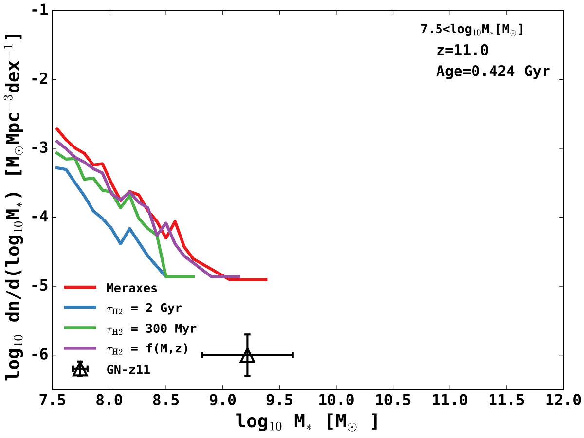 Figure 1
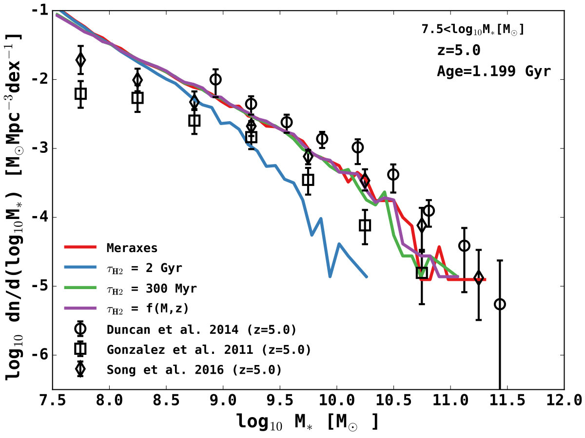 Figure 2
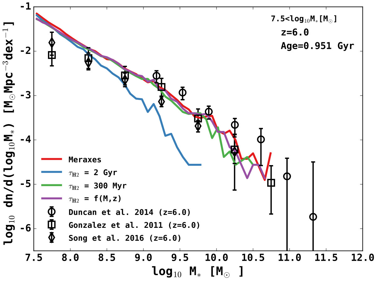 Figure 3
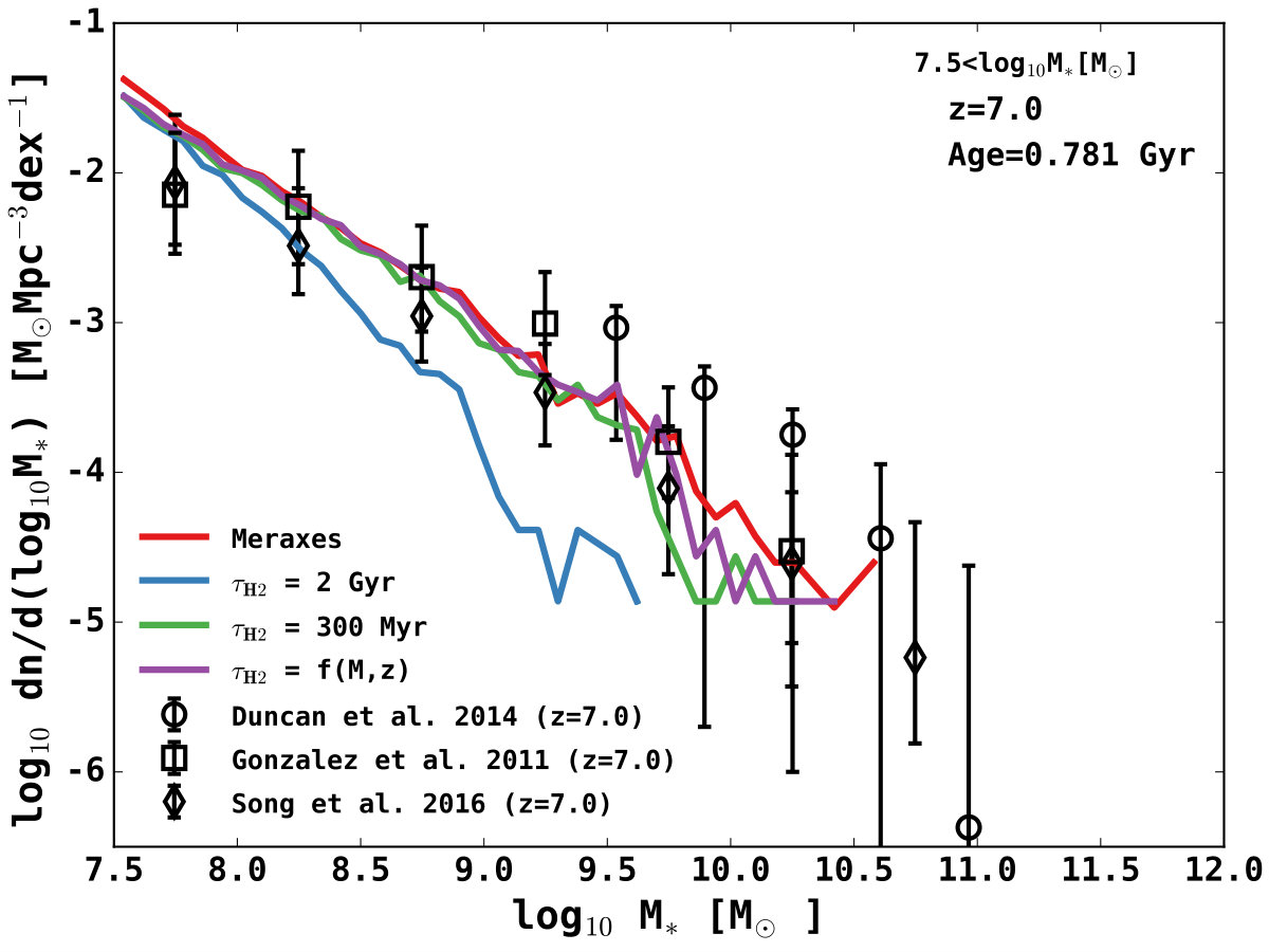 Figure 4
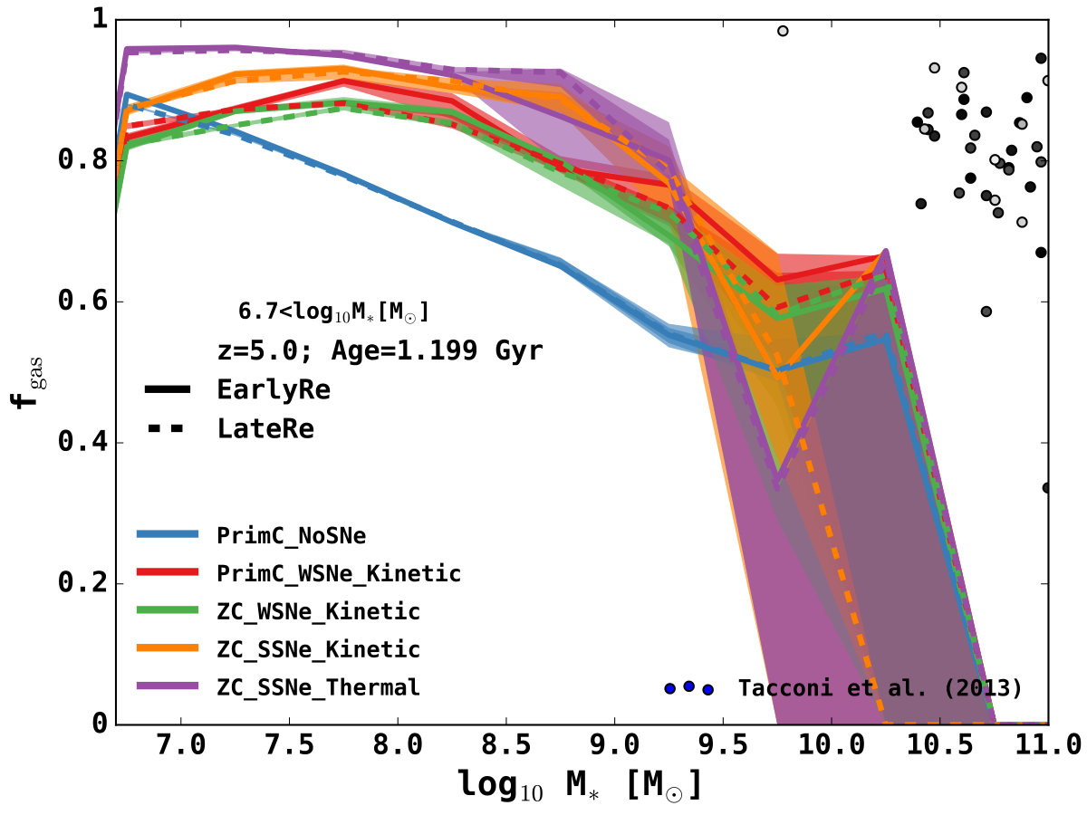 Figure 5
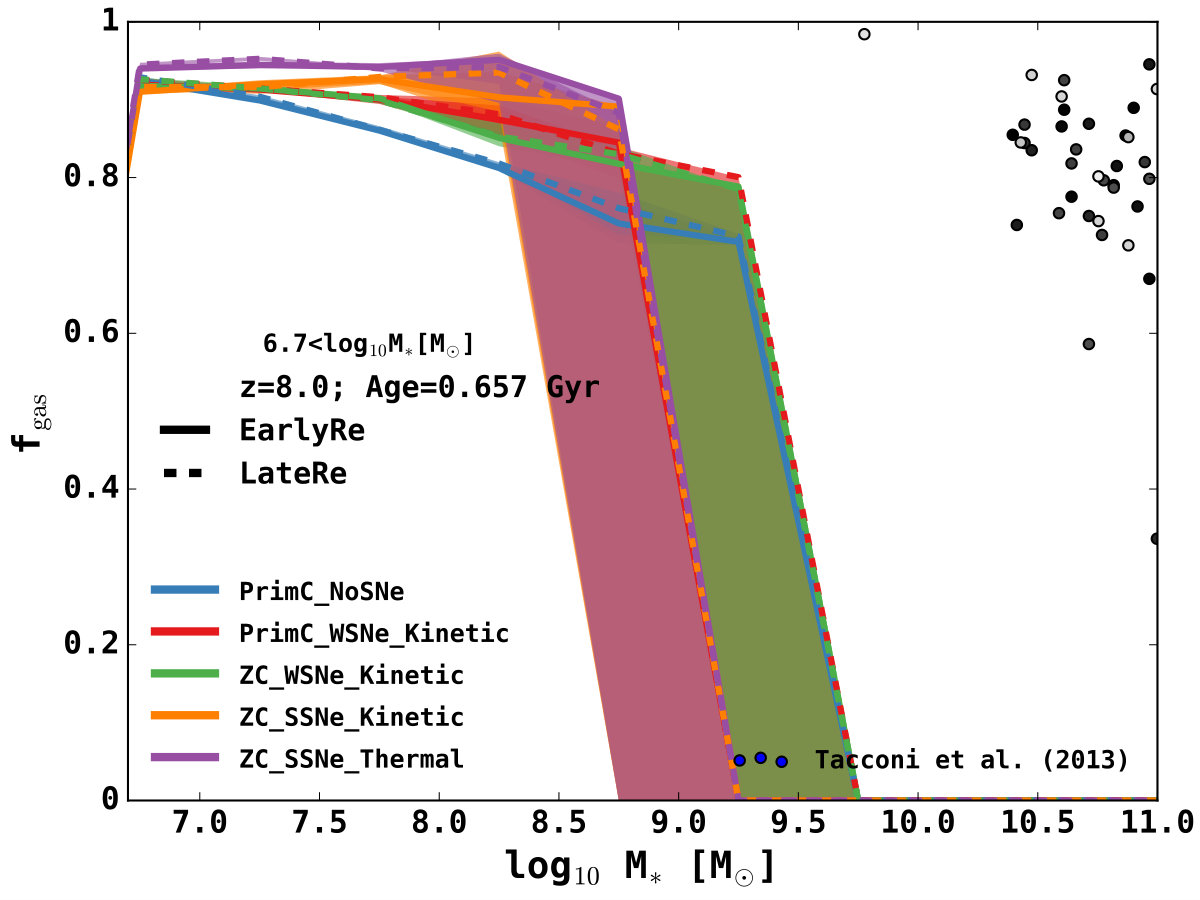 Figure 6
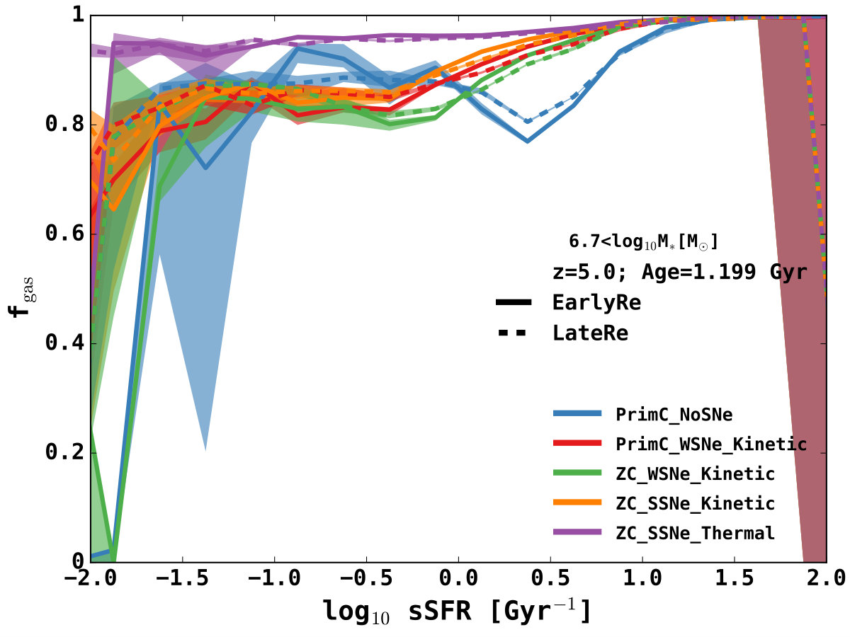 Figure 7
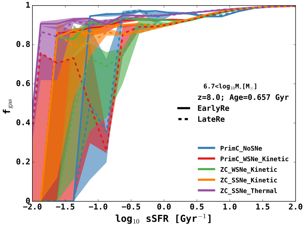 Figure 8
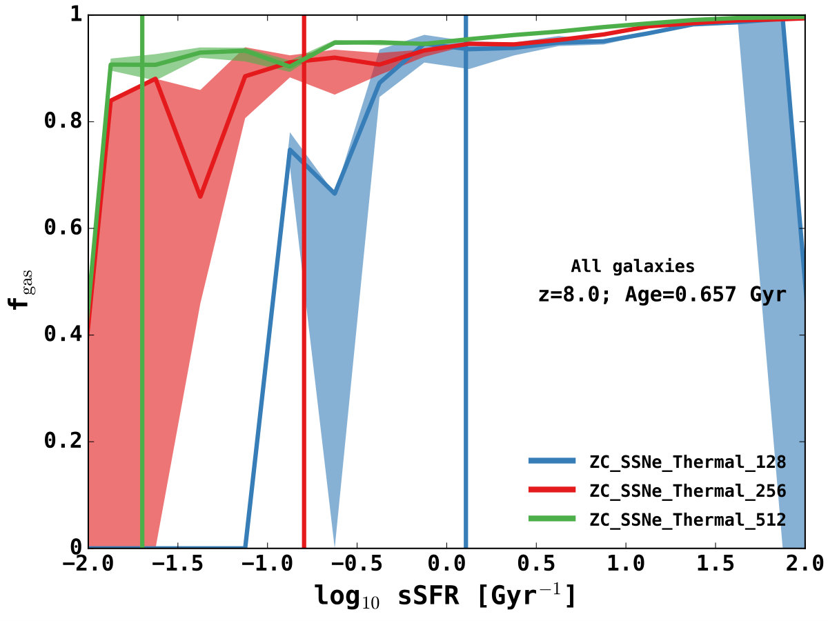 Figure 9
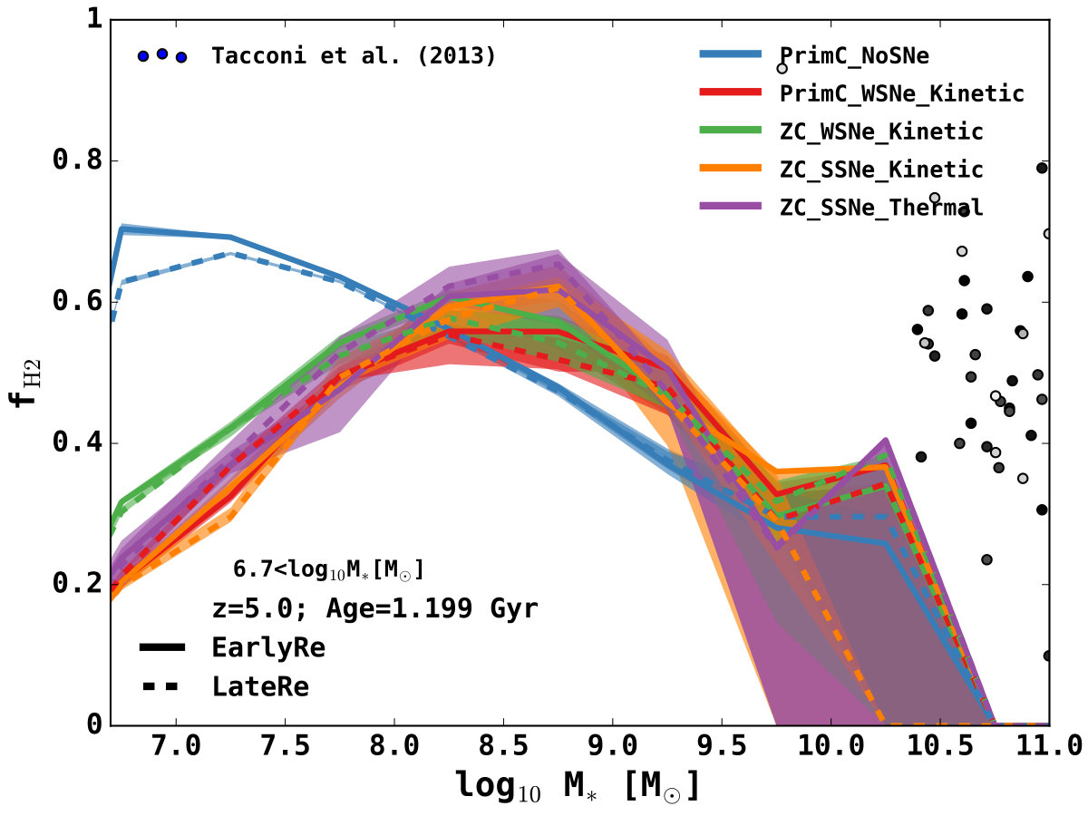 Figure 10
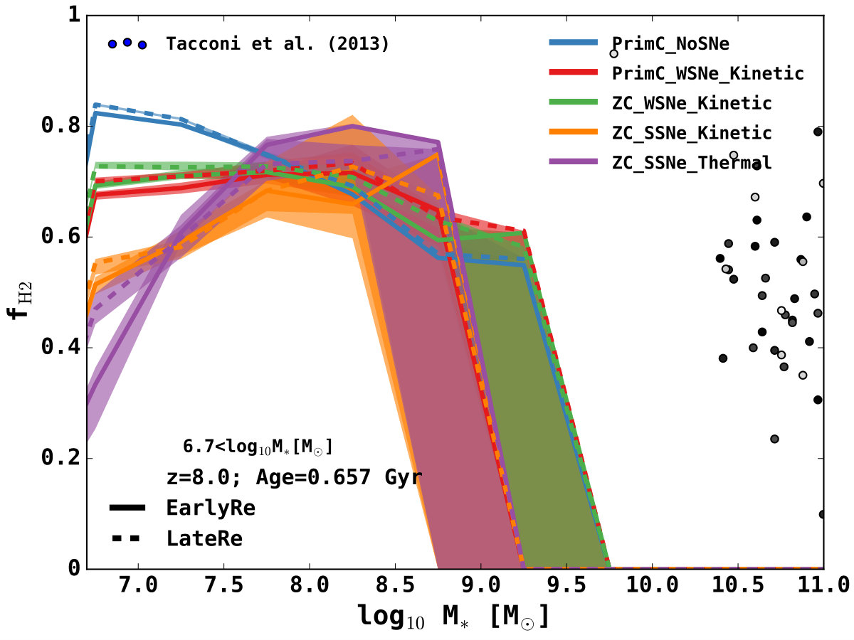 Figure 11
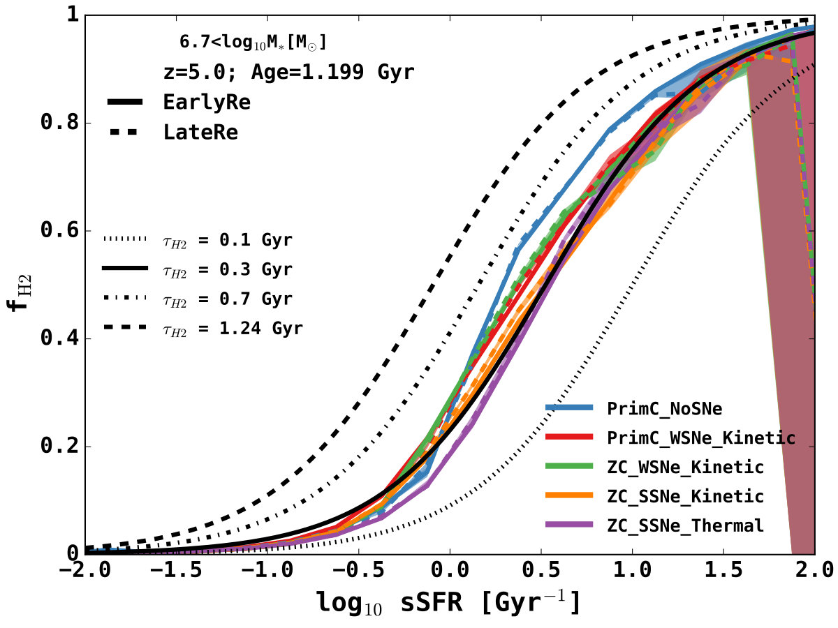 Figure 12
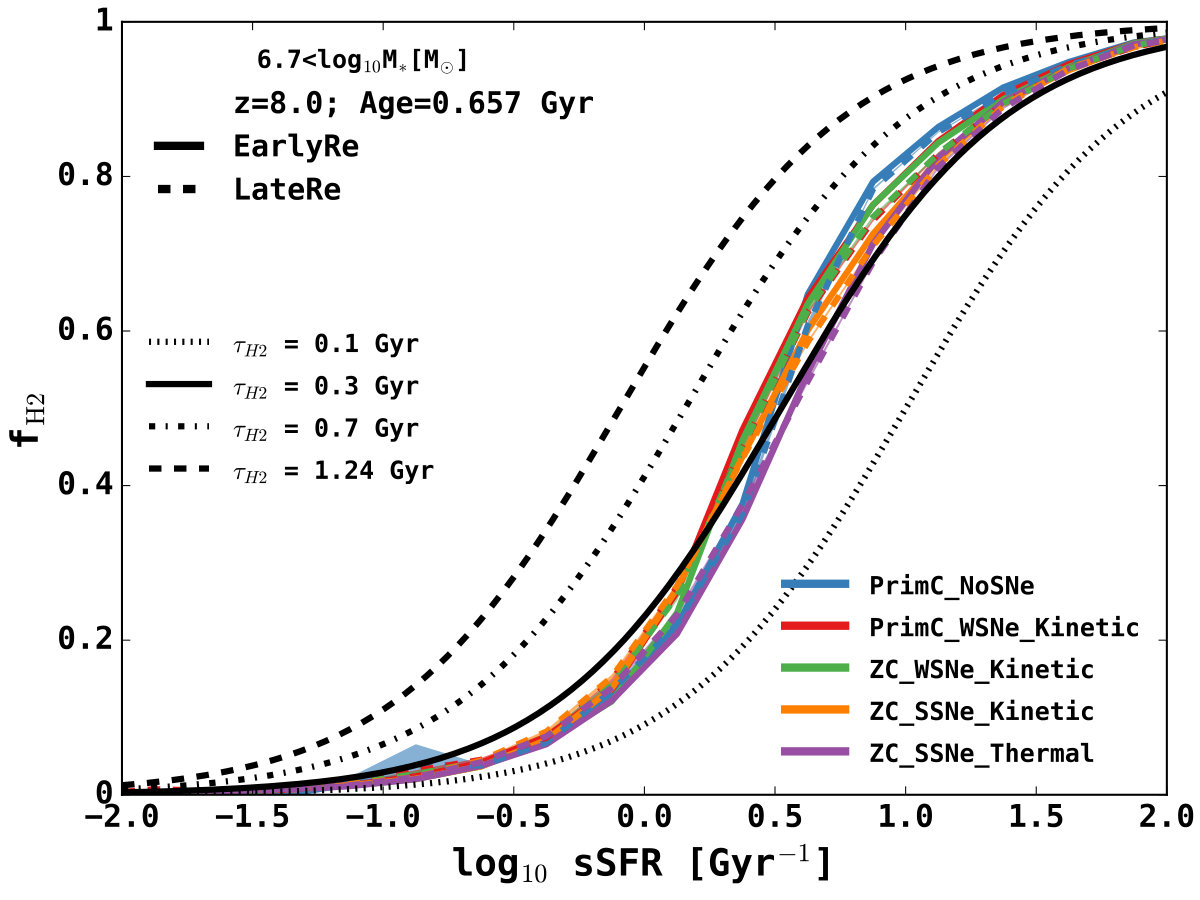 Figure 13
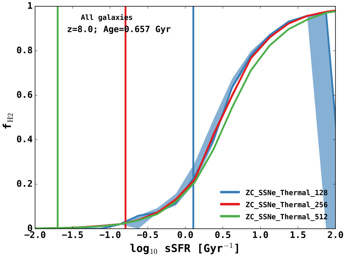 Figure 14
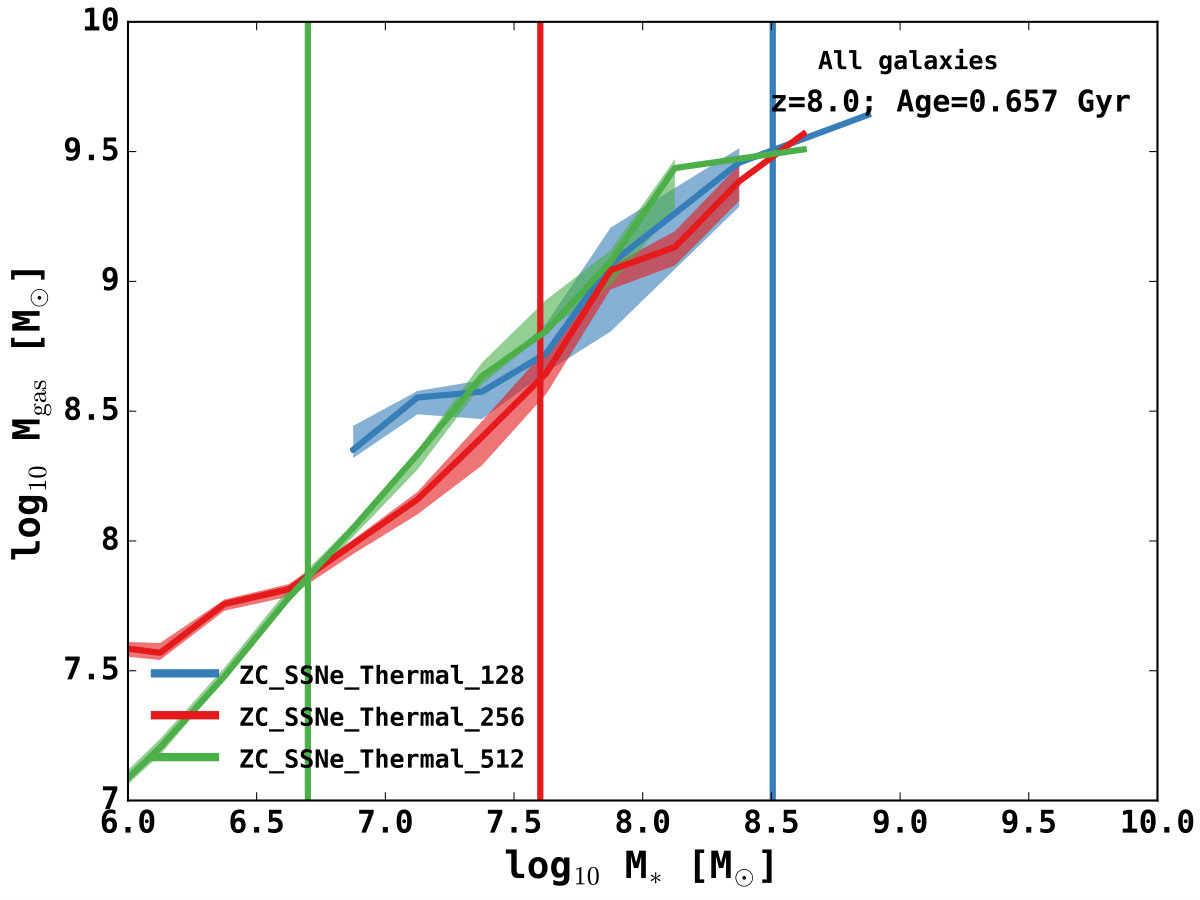 Figure 15
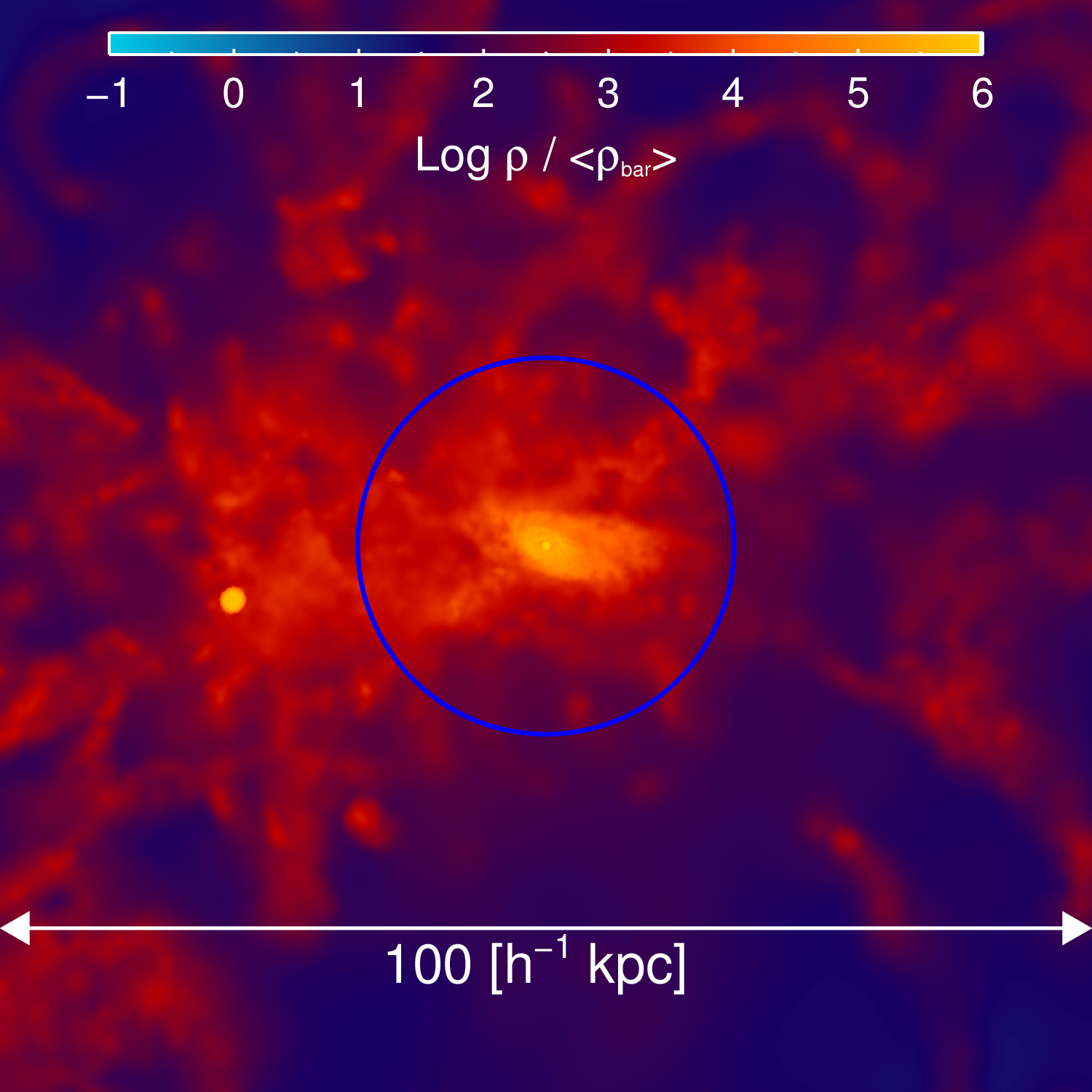 Figure 16
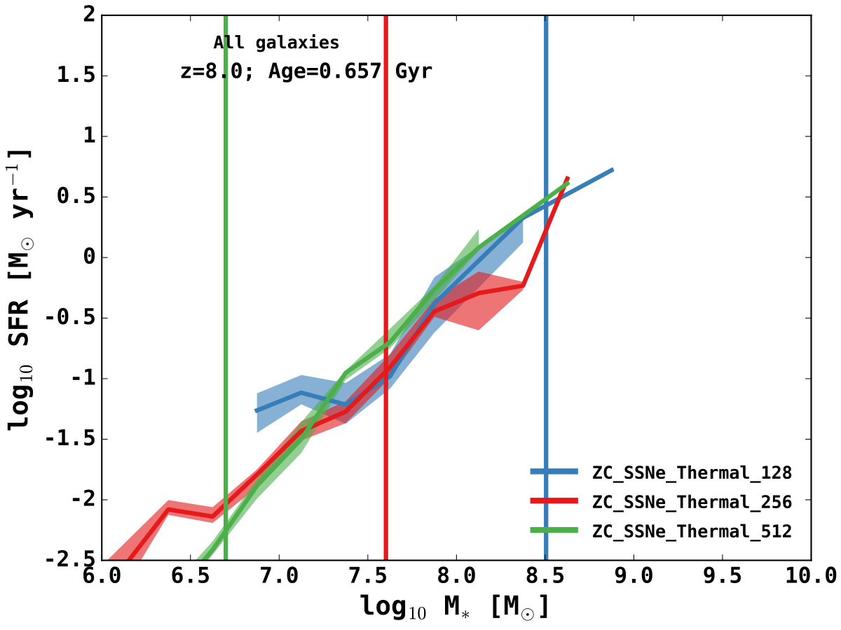 Figure 17
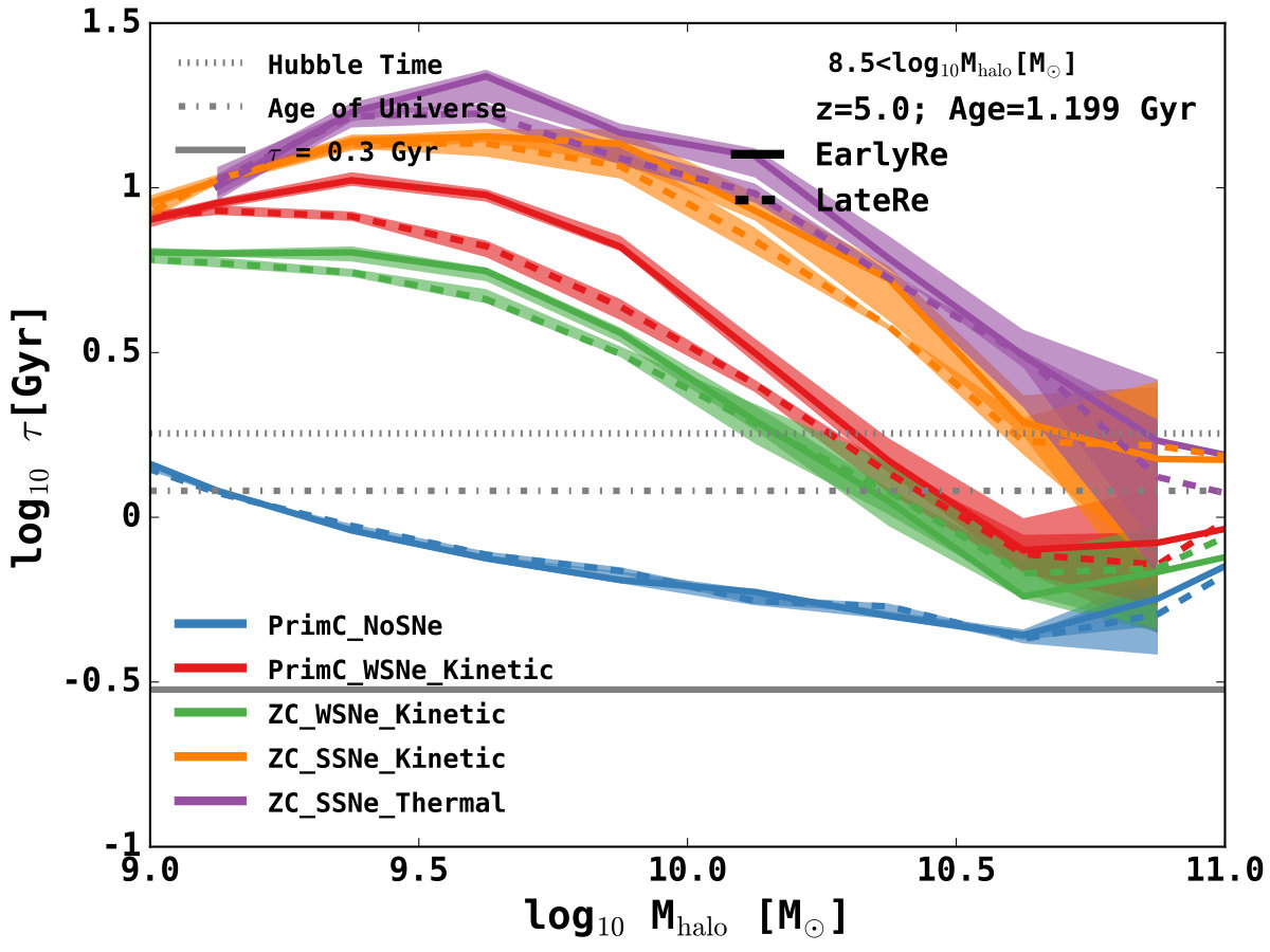 Figure 18
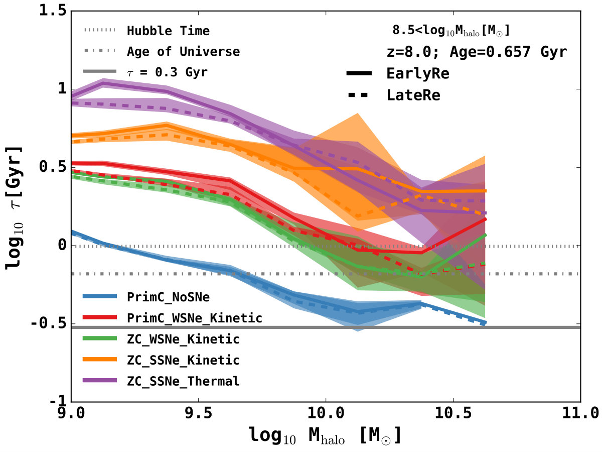 Figure 19
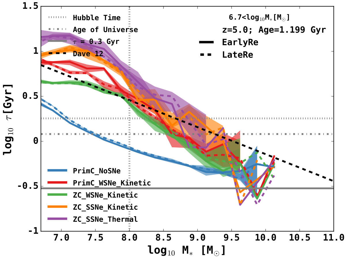 Figure 20
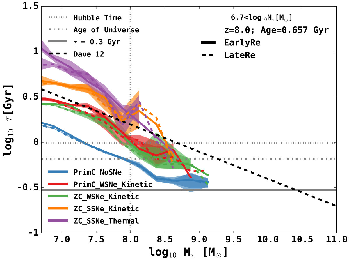 Figure 21
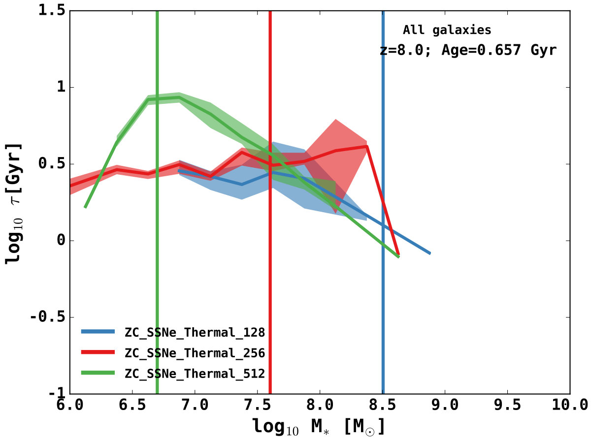 Figure 22
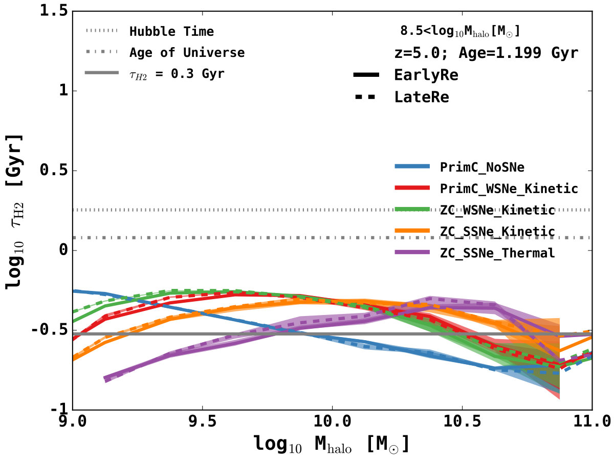 Figure 23
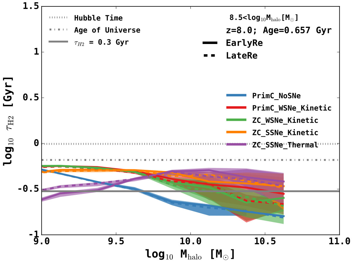 Figure 24
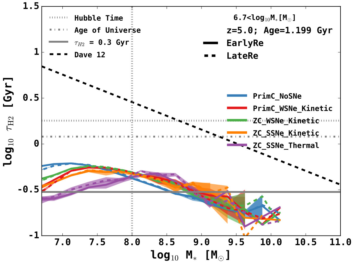 Figure 25
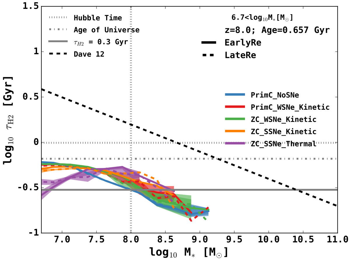 Figure 26
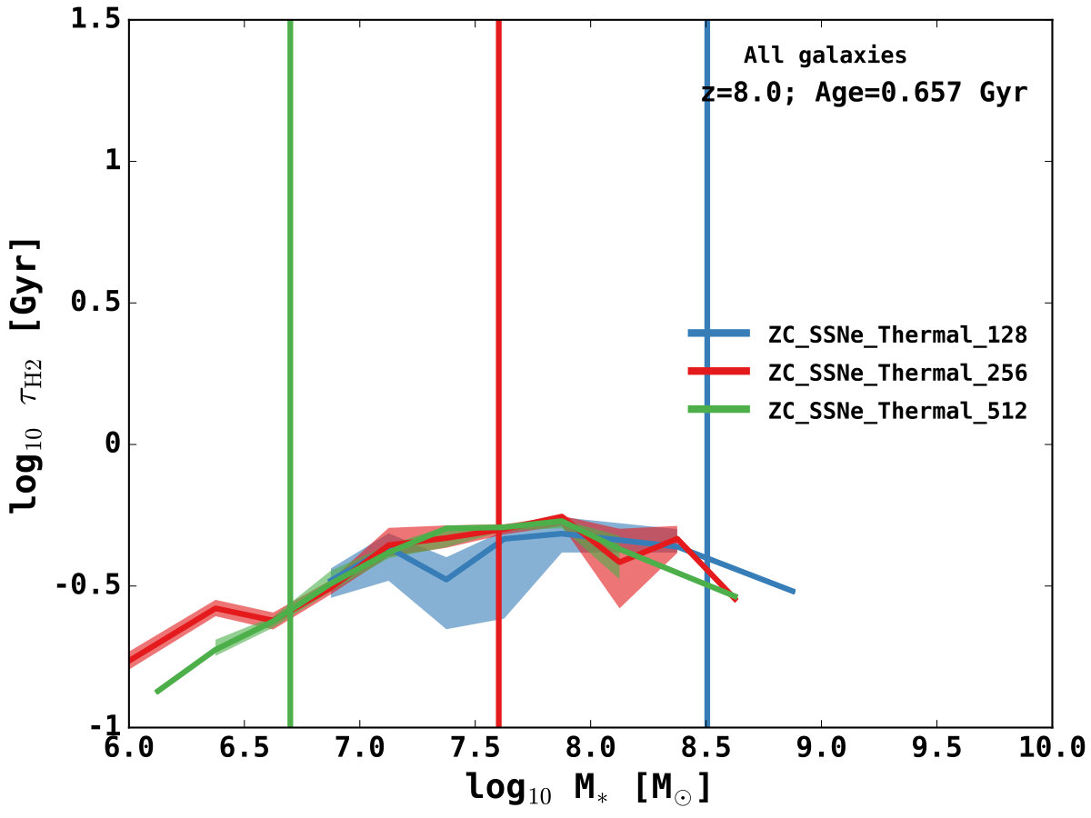 Figure 27
| Simulation | OWLS name | Brief description |
|---|---|---|
| PrimC_NoSNe | NOSN_NOZCOOL | No energy feedback from SNe and cooling assumes primordial abundances |
| PrimC_WSNe_Kinetic | NOZCOOL | Cooling as PrimC_NoSNe but with fixed mass loading of ‘kinetic’ winds from SNe |
| ZC_WSNe_Kinetic | REF | SNe feedback as PrimC_WSNe but now cooling rates include metal-line emission |
| ZC_SSNe_Kinetic | – | Strong SNe feedback as ZC_WSNe_Kinetic but using 100 per cent of available SNe energy |
| ZC_SSNe_Thermal | WTHERMAL | Strong SNe feedback as ZC_SSNe_Kinetic but feedback modelled thermally |
| Sim | ||||
|---|---|---|---|---|
| PrimC_NoSNe_EarlyRe | ||||
| PrimC_WSNe_Kinetic_EarlyRe | ||||
| ZC_WSNe_Kinetic_EarlyRe | ||||
| ZC_SSNe_Kinetic_EarlyRe | ||||
| ZC_SSNe_Thermal_EarlyRe | ||||
| PrimC_NoSNe_LateRe | ||||
| PrimC_WSNe_Kinetic_LateRe | ||||
| ZC_WSNe_Kinetic_LateRe | ||||
| ZC_SSNe_Kinetic_LateRe | ||||
| ZC_SSNe_Thermal_LateRe | ||||
| Sim | |||
|---|---|---|---|
| PrimC_NoSNe_EarlyRe | |||
| PrimC_WSNe_Kinetic_EarlyRe | |||
| ZC_WSNe_Kinetic_EarlyRe | |||
| ZC_SSNe_Kinetic_EarlyRe | |||
| ZC_SSNe_Thermal_EarlyRe | |||
| PrimC_NoSNe_LateRe | |||
| PrimC_WSNe_Kinetic_LateRe | |||
| ZC_WSNe_Kinetic_LateRe | |||
| ZC_SSNe_Kinetic_LateRe | |||
| ZC_SSNe_Thermal_LateRe |
Peer Reviews
No public reviews on file for this paper yet. If you reviewed it on a platform where reviews are public (OpenReview, ICLR, NeurIPS, ICML), you can paste yours below so the community can read it here.
Videos
No videos yet. Explain this paper in a talk, walkthrough, or lecture? Add one.
Dark-ages reionization and galaxy formation simulation - \Romannum9. Economics of reionizing galaxies
Alan R. Duffy1, Simon J. Mutch2, Gregory B. Poole2, Paul M. Geil2, Han-Seek Kim2, Andrei Mesinger3 and J. Stuart B. Wyithe2
1Centre for Astrophysics and Supercomputing, Swinburne University of Technology, Hawthorn, VIC 3122, Australia,
2School of Physics, University of Melbourne, Parkville, VIC 3010, Australia,
3Scuola Normale Superiore, Piazza dei Cavalieri 7, I-56126 Pisa, Italy
Abstract
Using a series of high-resolution hydrodynamical simulations we show that during the rapid growth of high-redshift () galaxies, reserves of molecular gas are consumed over a time-scale of almost independent of feedback scheme. We find that there exists no such simple relation for the total gas fractions of these galaxies, with little correlation between gas fractions and specific star formation rates. The bottleneck or limiting factor in the growth of early galaxies is in converting infalling gas to cold star-forming gas. Thus, we find that the majority of high-redshift dwarf galaxies are effectively in recession, with demand (of star formation) never rising to meet supply (of gas), irrespective of the baryonic feedback physics modelled. We conclude that the basic assumption of self-regulation in galaxies – that they can adjust total gas consumption within a Hubble time – does not apply for the dwarf galaxies thought to be responsible for providing most UV photons to reionize the high-redshift Universe. We demonstrate how this rapid molecular time-scale improves agreement between semi-analytic model predictions of the early Universe and observed stellar mass functions.
keywords:
methods: numerical – galaxies: evolution – galaxies: formation – galaxies: high-redshift – galaxies: star formation – cosmology: reionization.
1 Introduction
The study of galaxy formation at high-redshifts, , has undergone a revolution in the last several years with deep Hubble Space Telescope images, primarily the Hubble Ultra and eXtreme Deep Fields (Beckwith et al., 2006; Illingworth et al., 2013), enabling the study of galaxy populations in the first after the big bang. Additionally, new radio/submillimetre facilities such as the Karl G. Jansky Very Large Array, Atacama Large Millimeter/submillimeter Array and the Institut de Radio Astronomie Millimetrique Plateau de Bure Interferometer have provided resolved gas phase information at high-redshifts. Alongside the increase in observational data sets is a commensurate increase in theoretical efforts to explain these early galaxies’ high star formation rates (SFRs; e.g. Daddi et al., 2007; Noeske et al., 2007; Franx et al., 2008) and large gas fractions (e.g. Daddi et al., 2010; Genzel et al., 2010; Tacconi et al., 2010; Casey et al., 2011).
A general framework to explore galaxy growth is termed ‘baryon cycling’, whereby matter and energy flow into and out of a galaxy and the surrounding intergalactic medium. It has been argued through hydrodynamic simulations (e.g. Finlator & Davé, 2008; Davé et al., 2012) as well as scaling relations (e.g. Bouché et al., 2010; Dutton et al., 2010) that inflows and outflows will tend to balance, provided the SFR of a galaxy can adjust sufficiently quickly.
As discussed in the toy model of Schaye et al. (2015), an increase in the galaxy inflow rate, leads to a growth in the gas reservoir, , which can then form more stars . These stars then explode increasing the outflow of material as gas in the supernovae-driven winds. This interplay is described in
[TABLE]
The reverse is then also true. If inflow rates are less than the outflow rates, the gas reservoir decreases and star formation (SF) will begin to slow, thereby decreasing the resultant outflow rate. Ultimately, averaged over appropriate time-scales, outflows will balance inflows. In this regime galaxies are described by an equilibrium model (e.g. White & Frenk, 1991; Schaye et al., 2010; Lilly et al., 2013), also called the ‘bathtub model’ (Bouché et al., 2010; Davé et al., 2012). Another way to phrase this bathtub model is that galaxies are ‘supply-side’ limited and grow according to input gas flows.
If the system is in equilibrium then the gas reservoir changes () are negligible (Schaye et al., 2015) and thus . The resultant gas reservoir level in this picture does not directly depend on the feedback strength but rather is a consequence of the SFR that is needed to balance the inflows with outflows, provided the gas consumption time-scale is less than a Hubble time (Schaye et al., 2015). As shown by Krumholz & Dekel (2012), depending on the scaling relation used, star-forming galaxies at even modest redshifts () may not achieve this equilibrium state.
In this work, we will explore the ideas of gas consumption and replenishment at high-redshift during the Epoch of Reionization. The shorter Hubble time in this epoch may result in most galaxies being out of equilibrium. In particular, the gas reservoir term, , may not be negligible. Simple scaling arguments suggest that this may in fact be unavoidable at sufficiently high-redshift. In the (dense) early Universe galaxies can achieve high SFRs due to short dynamical times (). However, the gas may be even more rapidly replenished thanks to high infall rates, , which scale with cosmic infall as (e.g. Dekel et al., 2009; Correa et al., 2015a, b, c). The situation where local demand (SFR) cannot respond to increasing supply (gas) is termed a recession in economics.
We aim to explore early galaxy growth using high-resolution hydrodynamical simulations with various feedback schemes, determining the conditions under which early galaxies are supply-side limited. Studies of reionization require the physics of low-mass galaxy formation to be extended over volumes of . While these large volume hydrodynamical simulations are becoming increasingly available (e.g. Vogelsberger et al., 2014b, a; Schaye et al., 2015), they remain extremely computationally expensive. Traditionally, semi-analytic models (SAMs) have been used to explore the space of the various physical parameters in high-redshift galaxy formation (e.g. Benson et al., 2006; Lacey et al., 2011; Raičević et al., 2011; Zhou et al., 2013). These SAMs are computationally much cheaper and run as a post-processing step on an existing -body simulation, which can greatly exceed the hydrodynamical simulation in dynamic mass range probed for a comparable computational costs. However, in this work we hope to offer insight into emergent behaviour from the hydrodynamic simulations that can be incorporated into SAMs that study the Epoch of Reionization and thereby reduce their parameter space.
In Section 2 we describe the Smaug hydrodynamical simulations used in this work, and then explore the rate at which gas is consumed in the early galaxies in Section 3. We explore the dependence of the consumption time-scales on stellar mass and redshift in Section 4. The gas distribution as a function of mass is shown in Section 5, demonstrating that the vast majority of systems are indeed gas rich at high-redshifts. We then summarize our findings in Section 6, and discuss the implications of these findings for SAMs of early galaxy formation.
2 Simulation details
The Smaug simulation is a series of high-resolution hydrodynamical runs of a cosmological volume created as part of the Dark-ages Reionization And Galaxy Observables from Numerical Simulations (DRAGONS) project.111http://dragons.ph.unimelb.edu.au/ DRAGONS further includes the large -body Tiamat simulation (Poole et al., 2016) used to analyse large-scale dark matter (DM) structures during the era of first galaxy formation (Angel et al., 2016). The DM haloes then have galaxy properties applied with a bespoke SAM, meraxes (Mutch et al., 2016a), which includes coupled photoionization feedback through an excursion set scheme 21cmfast (Mesinger et al., 2011) to track reionization. Meraxes has successfully reproduced existing observations at high-redshifts () of the luminosity and stellar mass functions (Liu et al., 2016), sizes of galaxies (Liu et al., 2017) as well as predicted the reionization structure of the intergalactic medium around the growing galaxies (Geil et al., 2016).
There are a number of free parameters in the meraxes SAM. In this work we have investigated whether it is possible to use the emergent properties and scaling relationships from the explicitly modelled infall and outflow of the gas hydrodynamics in Smaug to inform the semi-analytics. In particular, we investigate the overall halo gas consumption times in early galaxies and demonstrate that gas consumption rates can be fixed independently of supernovae (SNe) feedback. This is potentially a substantial reduction in the freedom for early Universe models and ensures that maximum physical insight can be gained by comparing SAMs with the limited observations currently available.
2.1 Galaxy physics
The Smaug simulations (Duffy et al., 2014) were run with a version of gadget3, the -body/hydrodynamic code described in Springel (2005), with new modules for radiative cooling (Wiersma et al., 2009a), SF (Schaye & Dalla Vecchia, 2008), stellar evolution and mass-loss (Wiersma et al., 2009b), and galactic winds driven kinetically by SNe as given in Dalla Vecchia & Schaye (2008), or thermally SNe driven winds as implemented in Dalla Vecchia & Schaye (2012). The Smaug series of simulations all share the same initial conditions but are resimulated using numerous different physics models. These models are a subset of those tested in the OverWhelmingly Large Simulations series (OWLS; Schaye et al. 2010) which allows for robust investigation of the relative importance of each scheme, without exploring irrelevant physics to the high-redshift Universe (e.g. differing Type Ia SN models). These physics models have had success in reproducing observed galaxy properties at low, post-reionization, redshifts. The strong feedback schemes tested here have had success in reproducing the cosmic SF history (Schaye et al., 2010), as well as the high-mass end of the H i mass function (Duffy et al., 2012) at . Also, certain schemes reproduced the stellar mass function and specific star formation rates (sSFRs) at (Haas et al., 2013a, b). We briefly cover the simulation details here and summarize them in Table 1, but refer the reader to Duffy et al. (2010) and Schaye et al. (2010) for more explicit explanations of the physics, and Duffy et al. (2014) for greater detail of the Smaug simulations.
2.2 Initial conditions
Each simulation followed DM particles, and gas particles, where , within periodic cubic volumes of comoving length . The Plummer-equivalent comoving softening length is and the DM (gas/star) particle mass is . Lower resolution test cases with and were also run (see the Appendix). For all cases, we used grid-based cosmological initial conditions generated with grafic (Bertschinger, 2001) at using the Zeldovich approximation and a transfer function from cosmics (Bertschinger, 1995).
We use the Wilkinson Microwave Anisotropy Probe 7 year results (Komatsu et al., 2011), henceforth known as WMAP7, to set the cosmological parameters to [0.275, 0.0458, 0.725, 0.702, 0.816, 0.968] and .
After resolution testing (see the Appendix), we adopt a conservative cut on halo mass of , corresponding to DM particles, or on stellar mass of ( star particles) depending on the quantity explored. Note that all resolution limits are indicated on the plots used.
2.2.1 Radiative cooling
We follow the radiative cooling (and heating) prescription of Wiersma et al. (2009a) in which cooling (and heating) rates are assigned to each gas particle based on interpolated density and temperature tables from cloudy (Ferland et al., 1998). We track net radiative cooling rate for elements in the presence of the cosmic microwave background and (after reionization) a Haardt & Madau (2001) UV / X-ray background from quasars and galaxies. For our models named PrimC we only track this emission-line cooling from hydrogen and helium, while those named ZC have additional contributions from carbon, nitrogen, oxygen, neon, magnesium, silicon, sulphur, calcium and iron. The metallicity of each particle is calculated by weighting the nearest neighbours according to the smoothing kernel (Wiersma et al., 2009b). At high temperatures (seldom reached in Smaug for ) emission of bremsstrahlung radiation or inverse Compton scattering off cosmic microwave background photons dominates ionized gas cooling rates. Note that we do not model the expected molecular cooling from our simulations and instead calculate the molecular fractions in a post-processing scheme discussed in Section 2.2.3.
Note that we have modelled reionization as a background that is ‘switched on’ at () for simulations with EarlyRe- (LateRe-) ionization epochs. Such an instantaneous reionization is a relatively good approximation as reionized bubbles are comparable in scale (Wyithe & Loeb, 2004) to the simulation box sizes in Smaug. However, we use an optically thin approximation in which all gas particles are exposed to the background field. This will increase the fraction of gas that is impacted by photoionization feedback (ignoring self-shielding of dense gas) but underestimate the temperature immediately after reionization (e.g Wiersma et al., 2009a; Schaye et al., 2010). We note that local stellar sources of ionizing photons form in those regions that would be identified as self-shielded, thereby adding extra photons locally and in part mitigating this shielding. This mitigation means that the final neutral gas density distribution lies between the optically thin case and a cruder self-shielding approximation that lacks coupled radiative transfer, as shown in Rahmati et al. (2013).
2.2.2 Star formation
As gas cools, its density rises until reaching a critical point (with number density ) where it experiences instabilities leading to a multiphase medium and ultimately the formation of stars (Schaye, 2004). Our cosmological simulation lacks the resolution (as well as physics) to model molecular hydrogen formation and SF directly in multiphase regions. Therefore, as in Schaye et al. (2010) we have implemented222By setting we ensure that the Jeans mass and ratio of the Jeans length to the SPH smoothing kernel are independent of density (as demonstrated in Schaye & Dalla Vecchia 2008). an effective equation of state with pressure for gas above a critical hydrogen number density, . These star-forming gas particles are converted to stars according to a pressure-based star formation SF law, which was shown by Schaye & Dalla Vecchia (2008) to reproduce the observed Kennicutt–Schmidt law (Kennicutt, 1998). During SF, we convert one gas particle to one stellar particle as ‘spawning’ multiple generations of stars from a given gas particle leads to numerical artefacts and reduced effectiveness of SF feedback (Dalla Vecchia & Schaye, 2008).
We will explore the consequences of modifying the SF law (in particular with a metallicity-dependent threshold suggested in Schaye 2004) in a future publication, and emphasize that our conclusions in this work are restricted to an SF law with a fixed density threshold and parameter choice for the power law that reproduces the locally observed Kennicutt–Schmidt law.
2.2.3 Molecular hydrogen estimation
As previously noted, we do not have the required resolution to track the multiphase interstellar medium (ISM) within the cosmological volume of Smaug. Instead we use the empirical formalism described in Duffy et al. (2012) to estimate the molecular hydrogen fractions based on the pressure of the dense star-forming equation-of-state gas. We briefly describe this methodology here but refer the reader to Duffy et al. (2012) for more information.
We adopt the empirical scaling of the THINGS survey (Leroy et al., 2008) of a power-law relation between the surface density ratio of molecular-to-atomic hydrogen gas, , and the ISM pressure :
[TABLE]
By assuming that hydrogen in star-forming gas is essentially atomic neutral and molecular phases (with a negligible mass fraction of ionized hydrogen), this ratio then results in
[TABLE]
In practice, most of the star-forming gas at high-redshift is at such high pressures that the molecular component completely dominates the atomic neutral hydrogen fraction.
The pressure used in equation (2) is averaged over lengthscales of 800 and 400 pc for local galaxies and dwarf galaxies in Leroy et al. (2008), respectively. This is well above our resolution limit in Smaug, ensuring that these regions are well sampled. We note however that the empirical result is a local relation and therefore extending this to high-redshifts is potentially dangerous. More involved molecular hydrogen formation schemes, such as Gnedin & Kravtsov (2011) and Krumholz (2013) have been tested in Lagos et al. (2015) against the Duffy et al. (2012) prescription. Overall, Lagos et al. (2015) found that 82 (99) per cent of the molecular hydrogen identified by the Gnedin & Kravtsov (2011); Krumholz (2013) model was found in star-forming gas particles that Duffy et al. (2012), and hence this work, would by definition expect to contain molecular hydrogen.
The similarity between these schemes gives us confidence to continue with our simpler, empirically motivated prescription. We will explore more physically motivated schemes in future work, as Lagos et al. (2015) found that significant molecular hydrogen reserves can be found in non-star-forming gas as a result of more advanced molecular gas formation schemes (e.g. Gnedin & Kravtsov 2011 and Krumholz 2013) that depend on metallicity. In particular, even though we track metals in Smaug do not model the formation of molecular hydrogen on the expected dust grains from these metals and defer this for a subsequent simulation set.
2.2.4 Stellar evolution
We assume that each star formed is a single stellar population from a Chabrier (2003) initial mass function. Within the star particle we track the formation and timed release of metals from massive stars, as well as feedback (and chemical enrichment) from SNe Types Ia and II as described in Schaye et al. (2010). For the no-feedback model NoSNe we do not couple the SNe feedback to the gas as a test case. In the other simulations, after a delay time of , we assume that all massive stars (initial mass range ) have ended as core-collapse SNe releasing of energy. In this work we couple that resultant energy to the surrounding gas particles using one of the two techniques described below.
The first is a kinetic feedback scheme in which the nearest neighbouring gas particles of a newly formed star have a probability of receiving a ‘kick’ of wind velocity given by , where is the so-called mass-loading variable. For our weak feedback kinetic model WSNe_Kinetic, we adopt and that corresponds to of the available SNe energy being coupled into the wind. As was noted in Schaye et al. (2010), the value of per cent is reasonable as we do not model radiative losses in the Kinetic scheme. We also have tested the feedback scheme of Dalla Vecchia & Schaye (2012), which injects the energy stochastically into a neighbouring gas particle, and in principle accounts for all the energy of the SN explosion , a model we call SSNe_Thermal. To disentangle the impact that the additional energy of the explosion has in SSNe_Thermal with the different feedback implementation of Kinetic we ran a ‘strong’ kinetic model SSNe_Kinetic. This strong kinetic scheme has mass-loading and wind velocity that corresponds to all of the SNe energy, , coupled into the wind.
It is worth noting that we inject energy locally and never hydrodynamically decouple gas particles driven outwards in the wind. As shown by Dalla Vecchia & Schaye (2008), this is of key importance in creating realistic disc structures. An example disc galaxy from this particular simulation scheme is given in Fig. 1, showing the complexity of the gas distribution around newly forming systems that typically are dynamically unrelaxed at high-redshifts (Poole et al., 2016).
2.3 Power law
In this work, we fit an evolving power law to several quantities of interest (denoted here as ), with the following functional form
[TABLE]
where is either the stellar (or total halo) mass, with corresponding pivot mass , for a given redshift , normalized at . We explicitly state those situations when we restricted the stellar mass fitting range to be above as it is the high-mass end which is often best described by this power law. In practice, we take the quantity of interest over the redshift range of (in redshift intervals of ) and bootstrap the sample at each redshift creating samples that are binned across redshift with a uniform weighting applied during the least-squares (Levenberg–Marquardt) fit. We then record the solution to the bootstrap ensembles to estimate the confidence intervals around the best fit to the full sample.
3 Gas fractions
We now consider the predictions that equilibrium models, such as Bouché et al. (2010), Dutton et al. (2010) and Davé et al. (2012), suggest should exist between basic galaxy properties, in particular that early galaxies are more gas rich than low-redshift counterparts. The initial equilibrium relation, equation (1), describes the link between SF rising to consume inflows and driving outflows to achieve balance in the consumption of the primary raw material in a galactic economic system, that is, gas. We can separate the molecular gas fraction (tracing a denser star-forming phase of the gas) into two SF-related quantities
[TABLE]
with gas consumption time-scale and specific star formation rate . The molecular gas mass estimation is described in Section 2.2.3.
In the left column of Fig. 2 we explore equation (5) and find that, irrespective of feedback model, the simulations are approximately fit by a constant molecular gas consumption time-scale of (as we will see in Section 4.1 there is a weak stellar mass dependence). We note that this time-scale is shorter than any typically used or estimated for the low-redshift Universe. For example, Tacconi et al. (2013) find for main-sequence star-forming galaxies at while the same mass systems at consume gas over (Saintonge et al., 2011a). The analytic arguments of Forbes et al. (2014a) result in a cold gas consumption time for present-day haloes that decreases with total mass as (Forbes et al., 2014b), resulting in consumption time-scales that are several Hubble times for even our most massive objects in Smaug with .
We reiterate that in the left column of Fig. 2, we see little dependence on stellar feedback ranging from no SNe () with PrimC_NoSNe in blue to 40 per cent SNe energy () in PrimC_WSNe_Kinetic in red and ramping up to 100 per cent of the available energy () in ZC_SSNe_Kinetic in orange. The implementation of the feedback energy, be it kinetic or thermal, appears to have little effect as shown by the similarity between this ZC_SSNe_Kinetic curve in orange and ZC_SSNe_Thermal in purple. This near independence of the consumption time-scale to feedback is in agreement with other, low redshift, studies (e.g. Davé et al., 2011a, 2012; Somerville et al., 2015).
We also find little difference between the impact of metal emission-line cooling enhancing the consumption time-scale, as seen by comparing PrimC_WSNe_Kinetic in red and ZC_WSNe_Kinetic in green. This is unsurprising as it takes time for the metals formed in stars to be released into the halo gas and intergalactic medium. Additionally, halo virial temperatures must be sufficiently high () for heavy metal emission lines to be excited (Wiersma et al., 2009a) and thus lead to enhanced cooling of infalling intergalactic medium, or halo, gas.
To explore the best-fitting consumption time-scale in detail, we apply equation (5) at several redshifts of interest, using bootstrap sampling of the simulated haloes to estimate confidence intervals. As shown in Table 2, there is a small but significant dependence on the feedback model, with stronger feedback schemes demonstrating progressively shorter molecular consumption time-scales at all redshifts. The apparent contradictory trend of greater feedback resulting in shorter consumption time-scales is explored in Section 4.1.
The impact of reionization appears to be modest, resulting in consumption time-scales increasing by (or approximately per cent) seen by the close agreement of the LateRe and EarlyRe cases by . The decrease in SFR as a result of reionization was seen in Duffy et al. (2014) for the global SFR density (their Madau diagram, Fig. 6) where the exact redshift of reionization is not so important as the fact that it has occurred. We note that Smaug does not consider self-shielding and hence likely overestimates the (already modest) impact of reionization on this variable.
Overall, we find a remarkable convergence of consumption time-scales of for systems spanning the range of possible SNe feedback, enhanced metallicity cooling and even photoionisation feedback from reionization. This figure is intriguingly close to the gas consumption time-scale estimated by Lilly et al. (2013) based on their ‘gas regulator’ model for galaxies of when the Universe is old. However, we see little evidence in our simulations of their predicted rapid evolution in consumption time-scale (their Fig. 4) in the first billion years of cosmic time.
3.1 Sensitivity of total gas to sSFR
The tight and feedback-independent relation between the cold molecular gas phase and the specific star formation in the left column of Fig. 2 can be explored in the context of the total gas fractions (i.e. all gas gravitationally bound to the subhalo). Similar to equation (5) we have
[TABLE]
which we show in the right column of Fig. 2 for a range of redshifts.
Unlike molecular gas, there is no apparent correlation between the total halo gas fraction and sSFR. Instead, we see gas-rich galaxies, with , have sSFR that are effectively decoupled from their gas reservoir, exhibiting two to three orders of magnitude variation at all redshifts. This does not appear to fit into the picture of bathtub models, as this total gas fraction is likely dominated by material that lies far from the dense disc material where SF takes place. As a result, at high-redshift the vast amount of gas in a halo may play little role in setting the local sSFR. However, the exact transition from gas-poor/ultralow sSFR systems to gas-rich systems (with uncoupled stellar mass doubling times) is feedback dependent. Broadly speaking, a system with strong feedback is likely to transition to a gas-rich system at lower sSFR than a simulation without feedback. This is a result of that feedback preventing gas from forming stars. Overall, there appears to be a bottleneck in accumulated gas reserves transitioning into a useable form for the galactic ‘economy’. Observations (e.g. Catinella et al., 2010; Saintonge et al., 2011a, b) at low redshift have seen examples of gas rich systems exhibiting surprisingly low sSFRs or, equivalently, long consumption time-scales.
Our ability to determine the bottleneck in gas reserves being unable to transition to star-forming material is complicated by the lack of explicit molecular cooling in Smaug. However, argued by Lagos et al. (2015), who analysed molecular hydrogen in the EAGLE (Evolution and Assembly of GaLaxies and their Environments, Schaye et al. 2015) simulations (which share numerous numerical similarities with Smaug), this is a reasonable approach. First, the temperature of non-star-forming gas in the surrounding halo is greater than 11000K, far above the molecular cooling regime. Secondly, as found by Glover & Clark (2012), in the presence of even minor amounts of metals (in particular ), the contribution to cooling by is negligible at the high densities for SF. These densities are reached in Smaug and EAGLE alike even though gas is formally restricted to the atomic phase (Schaye, 2004). Finally, in hydrodynamical simulations such as Maio & Tescari (2015), which do incorporate non-equilibrium models for molecular hydrogen production, the impact of is greatest at higher redshifts () than we consider in this work.
In the next section, we investigate whether the approximate global consumption time-scale is truly uniform across all haloes or, instead, has a more complex dependence on the system it resides in.
4 Gas consumption dependences
We have shown that the typical consumption time-scale for star-forming gas in the high-redshift Universe is of the order of , far shorter than the Hubble time even during the Epoch of Reionization. In detail, however, this time-scale is potentially mass and redshift dependent. For example, we might expect smaller stellar mass systems to have lower SFRs and thus a much longer consumption time than larger systems, potentially longer than the Hubble time. Alternatively, at high enough redshift gas inflows may be too fast for SF ‘demand’ to ramp up to meet this supply, resulting in consumption times greater than the Hubble time at that epoch. Those systems that have consumption times less than a Hubble time would be described as supply-side limited, and those that have time-scales greater than the Hubble time would be demand-side limited. The bathtub / equilibrium models best characterize systems that are supply-side limited (i.e. have adjusted outflow rates, through SFRs, to the inflow rate). Therefore, the suitability of bathtub models can be indicated by the relative consumption time-scale to the Hubble time.
As demonstrated numerically in Davé et al. (2011b) and discussed in the analytic model of Davé et al. (2012), the consumption time-scale for ISM gas in haloes is given by
[TABLE]
This result was calculated by assuming a Kennicutt–Schmidt star formation law, in which SFR is set by the gas mass divided by the dynamical time of a disc. The dynamical time-scale then sets the consumption time-scale which, for a thin disc as given by the Mo et al. 1998 model, evolves as the Hubble time, . Finally, by taking the standard Kennicutt–Schmidt SF law relating gas surface density with the SF surface density, , and using an empirical relation between gas surface density and stellar mass, , Davé et al. (2011b) were able to formulate equation (7). We test whether this scaling holds for the high merger and accretion rate of haloes in the Epoch of Reionization explored by Smaug.
4.1 Cold molecular gas
In the left column of Fig. 3, we explore how the typical molecular gas consumption time-scale varies as a function of total stellar mass across a range of redshifts. We denote equation (7) with a black dashed curve and the Hubble time (age of the Universe) with dotted (dot–dashed) grey horizontal lines at the redshift in question. The fiducial time is indicated by the grey solid horizontal line.
In the left column of Fig. 3, it is clear that, at all stellar masses and redshifts considered, the consumption time-scale is less than the Hubble time. These time-scales are at least an order of magnitude faster than equation (7) suggests, although the total gas is in much better agreement (left column of Fig. 4). This is somewhat surprising as the molecular gas fraction is created from the equation of state, i.e. ISM, gas in Smaug and hence is closely tied to the ‘gas’ term adopted in Davé et al. (2012). We will return to this issue in the next section.
To explore the relative insensitivity of the molecular consumption time-scale to feedback more quantitatively, we fit the evolving power law of equation (4) over the redshift range of , with best fits (and bootstrap-estimated errors) shown in Table 3. Overall for a system of at , the molecular gas is depleted in just .
As shown in Table 3 there is a modest dependence on stellar mass, with for all simulations (in agreement with Davé et al. 2012). As a result of this sublinear dependence, consumption time-scales change by only factors of 2-3 across orders of magnitude in stellar mass. Due to the relatively limited population of large stellar mass systems in strong feedback models, the errors on their best-fitting solutions are rather large. Therefore, when we explore the use of a varying depletion time-scale (Section 6.1), we select the robustly estimated fits for ZC_WSNe_Kinetic_EarlyRe; however, all simulations have approximately the same qualitative behaviour.
Finally, we note that there appears to be a turnover at masses below our minimum fitting mass (particularly apparent for the strong feedback ZC_SSNe_Thermal model). We denote this as a dashed vertical line in the left column of Fig. 3 for clarity and note that choice of this cut-off is critical for the resulting power law behaviour. In Fig. 8, we explore resolution tests that show that this turnover is not apparently a simple consequence of numerical resolution. We leave this low-mass behaviour for zoom-in simulations to be presented in future work but note that the low-mass systems tend to have far less molecular gas available making the depletion time-scale of this gas relatively unimportant.
Overall, the consumption time-scale appears to have only a modest evolution across redshift () that was already suggested by the approximately constant consumption time-scale shown in Table 2. Overall, this is significantly less rapid evolution than the model of Davé et al. (2012) would suggest, which scales as [and hence in the matter era], but is in much greater agreement with the empirically determined time-scale evolution of Genzel et al. (2015).
In the right column of Fig. 3 we consider the consumption time-scales as a function of halo mass that now show greater variation as a function of feedback. The stellar mass independence of the various feedback schemes in the left column is revealed to be a result of a changing stellar-to-halo mass relation. This now explains the counterintuitive average consumption time in Section 3 in which strong feedback schemes more rapidly consume molecular gas reserves. The strong feedback systems have shorter consumption time-scales for low halo mass systems (as seen in the left column of Fig. 3) that dominate the sample size and hence global consumption time-scale for Fig. 2 and Table 2.
The overall picture of galaxies growing at high-redshift is one of rapid consumption time-scales that are insensitive to the feedback scheme used but not the stellar mass of the system they find themselves in. The situation of the gas reservoir surrounding the early galaxies is far more sensitive to the modelled feedback, as we explore in the next section.
4.2 Broader supply chains
We now consider the entire gas consumption time-scale in haloes, as given in Fig. 4, which is far longer than the corresponding molecular consumption time. We see that without feedback, PrimC_NoSNe, galaxies of have gas consumption time-scales less than a Hubble time at all redshifts considered. No-feedback models exhibit ‘run-away’ SF and are effectively supply-side limited. This means that a model without feedback effectively reaches equilibrium in the Epoch of Reionization for systems with such that the SFR traces the inflow accretion rate.
However, any feedback then moves the system to a quasi-regulated scenario in which the gas consumption time-scales are all larger than a Hubble time for , which in economics parlance is termed demand-side limited. For masses greater than this, we return to a supply-side limited scenario. We therefore conclude that the basic assumption of the bathtub model in which galaxies can adjust total gas consumption within a Hubble time does not apply for the dwarf galaxies responsible for providing most of the UV photons to reionize the high-redshift Universe (Duffy et al., 2014).
Although the normalization of the gas consumption time-scale is strongly feedback dependent, the stellar-mass-dependent scaling argued by Davé et al. (2012) appears to be a good description. This is actually surprising because the gas considered in our analysis is the entire gas distribution in the halo, and not the molecular hydrogen component traced by the Davé et al. (2012) model. As before, we fit the evolving power law of equation (4) to our simulations over the redshift range of , with best fits (and bootstrap-estimated errors) shown in Table 4.
For the no-feedback case we obtain a more modest mass dependence ( compared to ) to that found by Davé et al. (2012). For models with feedback there is a modest steepening of the relation from to as a function of increasing feedback. The overall normalization from the Davé et al. (2012) model agrees well with the kinetic SNe feedback scheme ZC_WSNe_Kinetic, which is most similar to their simulation, as detailed in Davé et al. (2011a, b).
Of all the physics schemes in Smaug the one that best matches the observed SFR function at high-redshift is ZC_SSNe_Thermal (Duffy et al., 2014) which has over twice the SNe energy available for feedback than both ZC_WSNe_Kinetic and the model of Davé et al. (2012). As shown in the left column of Fig. 4 in purple, this model also has over twice the gas consumption time-scale. This suggests that we are able to reproduce high-redshift observations by increasing total gas consumption time-scales through SNe feedback by disrupting and likely ejecting the halo gas that would otherwise transition into the cold star-forming phase.
The variation in the best-fitting evolutions of the consumption time-scales, , is a key sign that removal (and recycling from winds, e.g., Oppenheimer et al. 2010) of material can significantly impact the simple scalings presented in bathtub models of galaxy formation. Overall, however, models with feedback have to which is a far stronger redshift dependence than the no-feedback case, . Between these two extremes lies the scaling from Davé et al. (2012) which argued that the evolution is linear in Hubble time, i.e. as in the matter-dominated era at high-redshift.
The order of magnitude difference between the molecular gas and total gas consumption time-scales again demonstrates that there exists a bottleneck in high-redshift galaxies in converting infalling gas into the cold, dense star-forming phase (as also argued by Krumholz & Dekel, 2012). Broadly speaking, our total gas consumption time-scales at are similar to those observed in much larger starburst systems at lower redshift, , with Gyr (Daddi et al., 2010; Tacconi et al., 2010; Tacconi et al., 2013). This suggests that while galaxies during the Epoch of Reionization have similarly rapid consumption of gas to low-redshift massive systems, the reason is different with merger-induced starbursts replicating the ubiquitous inflow fed SFRs of the high-redshift Universe.
4.3 The 300 million year question
We now consider possible physical causes for the rapid and consistent molecular consumption time-scale of , as well as linear dependence on redshift. We emphasize that in the simulations presented in this study and in the following analysis we consider only a constant density threshold for SF of the form given in Schaye & Dalla Vecchia (2008).
We take the ratio of the molecular gas (calculated using the empirical scaling with local pressure of Leroy et al. 2008) as defined in equation (3) and the SFR, which is given by the pressure-based Kennicutt–Schmidt law (Kennicutt, 1998) derived by Schaye & Dalla Vecchia (2008):
[TABLE]
with ratio of specific heats , the gas fraction that is effectively unity for our systems, and set by the observed Kennicutt (1998) relation. The pressure for dense (i.e. above ) star-forming gas is governed by a polytropic equation of state as our simulations lack the resolution to track this otherwise multiphase medium
[TABLE]
where , . The resultant molecular consumption time for a single gas particle is then the ratio of equations (3) and (8), giving
[TABLE]
We can then determine that a consumption time-scale of corresponds to gas with particle density , which is an extremely high number density for galaxies at low redshift but similar to giant molecular clouds in their self-bound collapse phase (Krumholz et al., 2012). The SF in the central regions of the galaxies at high-redshift is effectively an enormous molecular cloud, with over a third of the mass in the most massive systems above this density at . We note that the median logarithmic density across all star-forming particles is of the order of , which corresponds to consumption time-scales only twice that of the highest density gas. That fact that feedback can make little difference to the molecular gas consumption time-scale is reasonable given the extraordinarily high density of the gas contributing to this phase.
We can also explore the redshift dependence of the consumption time-scale. We start by using the Schaye (2004) calculation for the central particle number density of a self-gravitating disc assuming an exponential surface profile,
[TABLE]
where the mass of the disc with characteristic disc scalelength , with spin parameter at high-redshift (Angel et al., 2016). We further assume the sound speed for an isothermal gas at , as the molecular weight for primordial neutral gas and is the mass of hydrogen. Using the stellar-to-halo mass relation () from Mutch et al. (2016a) we then can show that haloes of stellar mass can be expected to have central densities of the order of , which is exactly what the Smaug simulations show, and that a consumption time-scale of requires.
From equation (11), we can see that the number density naturally scales as assuming constant fraction of disc length to virial radius (). We can then expect that our star-forming gas pressure, equation (9), in the disc will scale as . This pressure-redshift scaling then leads to a molecular gas consumption time-scale (equation 10) that depends on redshift as . This result is in excellent agreement with our fits in Table 3 and our adopted case of ZC_WSNe_Kinetic_EarlyRe with . Overall, the hydrodynamical simulations suggest a varying consumption time-scale, we will explore the incorporation of this time-scale in SAMs of the Epoch of Reionization in Section 6.1.
5 Gas distribution
With the increasing sensitivity of mm-wavelength facilities, such as ALMA and IRAM, there are now statistical samples of the gas contents of galaxies at moderately high-redshifts, in particular we will compare our simulations to Tacconi et al. (2013) for galaxies. A key result from bathtub models is that high-redshift galaxies will be gas rich, and only in the most massive systems can the gas reserves be depleted faster than they are replenished by infall (a prediction that we confirmed in the last section).
In the left column of Fig. 5, we show the molecular gas fraction in haloes as a function of stellar mass for several high-redshift examples. Overall, systems that exhibit run-away SF as they have no stellar feedback (PrimC_NoSNe in blue) are the most gas rich at low stellar masses. This is the same result we saw for the consumption time-scale in the left column of Fig. 3, and shows that at low masses SFRs simply cannot respond to the rapid inflow of material. Therefore, gas-rich systems are demand-side limited. The effect of increasing stellar feedback is that gas is removed in lower mass systems. Above , all simulations show the same decrease of gas fraction with increasing stellar mass, with systems per cent less gas rich than at .
From Davé et al. (2011b), the expected scaling at low redshifts is approximately , which is far steeper than we see at high redshift, confirming the picture that high-redshift systems are more gas rich than low-redshift counterparts. Indeed, it has been argued that gas-poor systems at late times are a natural consequence of the bathtub model because the accretion rate drops more rapidly with redshift than the SFR, implying that the gas reservoir is slowly used up.
Intriguingly, the high molecular fractions from Tacconi et al. (2013) are only reproduced in our high-redshift objects with an order of magnitude lower stellar mass. To match their observations would require the characteristic stellar mass scale at which molecular gas fractions peak to increase with decreasing redshift. Thus, while it may be possible to match the high gas fraction results in the lower redshift observations of Tacconi et al. (2013) by a secular evolution in the galaxy populations, it is unclear what would drive this trend. One possible mechanism could be mergers bringing in significant new material, as well as increasing the pressure such that the molecular to atomic gas ratio increases. Unfortunately, we cannot test this in Smaug as the simulation does not continue below .
Although there is significant scatter in the gas fraction with feedback models, we see a modest trend that stronger SNe typically result in more gas-rich systems. This is a consequence of increased feedback energy requiring fewer exploding stars to suppress SF in the surrounding gas. In other words, a given mass of stars formed in a strong feedback model will eject more gas from the diffuse halo reservoir, preventing that gas being locked up in stars and increasing the gas fraction. We note that as the gas fraction is defined as gas mass divided by the total gas and stellar masses, a modest reduction in gas mass is less significant in reducing the gas fraction than allowing (even some of) that ejected gas to form stars. It is entirely possible for some of this ejected gas mass to be later re-accreted billions of years later as a wind-mode recycling of material (e.g. Oppenheimer et al. 2010) but not enough time has elapsed by the end of the Epoch of Reionization for this to occur.
In conclusion, the simplest interpretation of the difference in consumption time-scales of molecular gas (Fig. 3) and total gas (Fig. 4) at fixed halo mass is that the amount of star-forming gas (from which the molecular gas is entirely sourced) is suppressed relative to the halo gas mass. The challenge with this picture is that feedback is expected to remove lower density material preferentially to the dense, star-forming gas. We are therefore left with the conclusion that feedback has acted to restrict the inflow of gas into the dense phase, either through direct heating of star-forming gas, or more likely disruption and possibly ejection of the halo material transitioning to that phase.
6 Discussion
Before discussing how our results might be used to improve the SF recipes in SAMs for galaxy formation at high-redshift we first summarize our main findings.
We have found that Smaug hydrodynamic simulations predict the molecular gas fraction to strongly correlate with the sSFR, with a typical molecular consumption time-scale of (as given in the left column of Fig. 2) irrespective of feedback. In detail this time-scale has a modest dependence on feedback, with shorter consumption time-scales for increasingly strong SNe feedback, as well as decreasing redshift, as shown in Table 2. Typically, reionization acts to increase the consumption time-scale by 10-20 per cent (). We found no such trends with the total gas fraction. For values above ultralow sSFR (with doubling times an order of magnitude longer than the Hubble time), all objects were similarly gas rich () irrespective of their growth rate.
We then explored in greater detail the dependences of the consumption time-scales. As shown in Fig. 3 (and with best fits in Table 3), the molecular gas consumption time-scale depends on stellar mass and redshift. However, we find that at all masses explored the star-forming (molecular) gas phase is consumed far more quickly than a Hubble time and in a manner independent of the SNe feedback physics. As a result, SF in these systems is constrained by how quickly infalling gas is converted into the molecular phase.
The situation is greatly changed when we consider the total gas consumption time-scales, shown in Fig. 4 and best fits in Table 4, which is strongly dependent on the feedback model. We find that consumption times increase at fixed stellar mass and redshift as a function of increasing feedback energy. This is distinct from bathtub model predictions (which to first order are feedback-independent time-scales) and is a critical reminder that the amount of gas is not so important as the state of that gas, even in a cold and dense early universe.
6.1 Implications for semi-analytic galaxy formation models
Implementation of findings from this investigation in SAMs of the Epoch of Reionization depend on the particular SF parameterisation. In this section, we consider the SAMs presented in Mutch et al. (2016a, meraxes) and Lagos et al. (2011, galform).
The original galform model that adopted (Cole et al., 2000) could be readily adaptable to the simple constant consumption time-scale suggested in this work with . Indeed, the SF scheme in recent SAMs has been updated to include insights from observations showing that the density of SF correlates strongly with the molecular gas density (e.g. Blitz & Rosolowsky, 2006; Leroy et al., 2008). These results have triggered significant activity in SAMs aimed at including an explicit treatment for the transition from atomic to molecular hydrogen, and molecular hydrogen based SF laws (Fu et al., 2010; Guo et al., 2011; Lagos et al., 2011; Somerville et al., 2015; Wolz et al., 2016). For example, Lagos et al. (2011) and Wolz et al. (2016), a modification of the SAGE model presented in Croton et al. (2016), use a pressure-based transition of neutral to molecular hydrogen (Blitz & Rosolowsky, 2006), similar to the molecular mass calculation of Duffy et al. (2012) that we have adopted in Smaug. The Wolz et al. (2016) implementation of SAGE and the SAMs considered in Lagos et al. (2011) use a constant consumption time-scale , constrained from local Universe observations in Leroy et al. (2008) and Bigiel et al. (2011).
For meraxes, the SFR is (Mutch et al., 2016a, their equation 7) where discs of have typical dynamical time-scales for and a fiducial SF efficiency per dynamical time of for cold gas mass above a critical threshold . This prescription, which follows Croton et al. (2006, 2016), has an effective overall gas consumption time-scale of at which at first glance is approximately 50per cent longer than the time-scale we find in Smaug (Fig. 2). However, due to the difference in gas mass definitions, where only gas above the critical density is converted per consumption time, the meraxes gas reservoir is even less rapidly used for SF than the simple comparison of time-scales would suggest. By moving to a more explicit molecular gas mass calculation, rather than cold gas above a critical threshold, SAMs like meraxes could directly use the results from Smaug to more physically model SF.333We note that such a direct comparison between techniques is potentially complicated by baryonic suppression of halo growth when gas physics is explicitly modelled as shown by Qin et al. (2017). This is particularly an issue for high-redshift dwarf galaxy merger trees generated from -body simulations in which halo mass can be significantly overestimated. This direct comparison is further explored in Qin et al. (in preparation). The current meraxes formalism, while successfully able to reproduce a range of SFR and stellar masses across redshifts, is a phenomenological relation and it is desirable to construct a more physical model.
Based on this discussion, we implement a new SF law informed by Blitz & Rosolowsky (2006) to modify meraxes following Wolz et al. (2016) for three different molecular consumption time-scales. All other parameters remain as constrained by Mutch et al. (2016a). The first two tests are with constant time-scales; a default appropriate for low redshifts, and as suggested by Smaug for high-redshifts. We also test a variable consumption time-scale that is a function of redshift and stellar mass according to equation (4) and use the best-fitting models presented in Table 3. Due to the similarity in the qualitative behaviour of all simulations above in stellar mass, and the relatively fewer systems in the SSNe feedback schemes to constrain the fit, we choose one of the more robustly constrained schemes. In this case, we have tested ZC_WSNe_Kinetic_EarlyRe with that we note if extrapolated to the present day for low-mass systems at gives a similar result of to that found by Leroy et al. (2008).
We compare the resulting stellar mass function from the different molecular consumption time-scales in Fig. 6. It is clear that the shorter time-scale of recovers the observations of Song et al. (2016) when compared against the low-redshift calibrated value of and is also in excellent agreement with the highly successful, but phenomenological, original meraxes formalism. In particular, it is able to match the observed low stellar mass downturn () at high-redshift () of González et al. (2011) and Duncan et al. (2014). The shorter time-scale that varies with mass and redshift is required to create an object as massive as ‘GN-z11’ (Oesch et al., 2016) at such high-redshift (top left-hand panel of Fig. 6) as was found in the original meraxes model (Mutch et al., 2016b). Therefore, we conclude that adopting such a time-scale represents a marked improvement over longer time-scales set by present-day observations. However, we will show through Markov chain Monte Carlo exploration of the parameter space (Mutch et al. in preparation) that the standard meraxes SF law and stellar feedback implementation is unable to produce the observed flattened stellar mass function at , while still allowing objects such as ‘GN-z11’ to form in time. We leave the exploration of further observational consequences of the suggested improvement to semi-analytic modelling at high-redshift to future work (Kim et al. in preparation).
7 Conclusion
During reionization, galaxies are still so young that the recycling of gas or metal enrichment has not had time to significantly impact their growth. However high-redshift galaxies, while lacking that complexity, are not in equilibrium and do not grow as expected from the bathtub model. We find that early galaxies grow with a molecular gas consumption time-scale of at independent of feedback. The redshift-dependent result, in agreement with simple exponential disc scaling arguments, of naturally leads to a time-scale of at in good agreement with local Universe predictions. It also greatly improves the agreement between SAM predictions and observations of the stellar mass function at higher redshift.
We found that there is no simple relation for the total gas consumption time-scales as gas-rich galaxies can have sSFRs that differ by two to three orders of magnitude at fixed gas fraction, irrespective of feedback. This suggests that early galaxies were not able to raise their growth rates as fast as new material arrived.
In contrast to the standard view of a ‘booming’ early Universe, galaxies of this time were actually in recession, with bottlenecks in transitioning inflowing gas to the ISM preventing demand in the galactic economy from responding to the overabundance of supply. The period of rapid galaxy growth comes later, when galaxies move from demand-side limited recession to a one that is supply-side limited and close to the Universe we live in today.
Acknowledgements
ARD would like to thank Caitlin Casey, Katie Mack and Kristian Finlator for stimulating discussions, Claudio Dalla Vecchia for his SNe feedback models, as well as Chris Power and Doug Potter for their efforts with initial conditions. JSBW acknowledges the support of an Australian Research Council Laureate Fellowship. This work was supported by the Flagship Allocation Scheme of the NCI National Facility at the ANU, data storage at VicNodes, generous allocations of time through the iVEC Partner Share and Australian Supercomputer Time Allocation Committee. ARD gratefully acknowledges the use of computer facilities purchased through a UWA Research Development Award. We would like to thank the Python developers of matplotlib (Hunter, 2007), CosmoloPy (http://roban.github.com/CosmoloPy) and pynbody (Pontzen et al., 2013) for easing the visualization and analysis efforts in this work.
Appendix A Resolution Testing
We have extensively explored resolution tests for the Smaug simulation series, focusing on comparing the increasingly well-resolved models with gas and DM particles in the same initial conditions of cubic volumes of comoving length . In our tests, we explored resulting in Plummer-equivalent comoving softening lengths of and DM (gas) particle masses of , respectively.
We explored mass functions for all our basic properties and found that baryonic processes, , were resolved at high-redshift above
[TABLE]
where depends on the variable of interest. Stellar, gas and molecular masses have respectively while . We also found that a conservative cut on halo mass of resulted in most derived quantities for those larger haloes being consistent.
We show an example resolution test in Fig. 7 with the SFR (gas mass) shown against stellar mass in the top (bottom) panel. The vertical lines are the cuts from equation (12) and show that the systems are well behaved above these limits.
It is more difficult to determine the exact numerical convergence, or mass cut-off, for the other derived quantities explored in this work. In Fig. 8, we see that the characteristic turnover of the consumption time-scale at low stellar mass (left column of Fig. 3) appears to be independent of resolution. The overall gas consumption time-scale (bottom panel) suffers significantly more obviously from numerical issues; however, the minimum stellar halo mass we consider for our fits of is well above even the most conservative of estimates.
As we see in Fig. 9 the total gas fraction (bottom panel) has a more obvious numerical resolution limit than that of the molecular gas (top panel). The increasing resolutions allow the gas fraction to be sampled at ever lower sSFR, with scaling given by equation (12). The case for the molecular gas fraction (as with Fig. 8) appears to be less obviously affected by resolution. This agreement should not be overly surprising as the consumption time-scale is the common variable between these two tests.
The reference list from the paper itself. Each links out to its DOI / PubMed record.
- 1Angel et al. (2016) Angel P. W., Poole G. B., Ludlow A. D., Duffy A. R., Geil P. M., Mutch S. J., Mesinger A., Wyithe J. S. B., 2016, MNRAS , 459, 2106 · doi ↗
- 2Beckwith et al. (2006) Beckwith S. V. W., et al., 2006, AJ , 132, 1729 · doi ↗
- 3Benson et al. (2006) Benson A. J., Sugiyama N., Nusser A., Lacey C. G., 2006, MNRAS , 369, 1055 · doi ↗
- 4Bertschinger (1995) Bertschinger E., 1995, Ar Xiv Astrophysics e-prints,
- 5Bertschinger (2001) Bertschinger E., 2001, Ap JS , 137, 1 · doi ↗
- 6Bigiel et al. (2011) Bigiel F., et al., 2011, Ap J , 730, L 13 · doi ↗
- 7Blitz & Rosolowsky (2006) Blitz L., Rosolowsky E., 2006, Ap J , 650, 933 · doi ↗
- 8Bouché et al. (2010) Bouché N., et al., 2010, Ap J , 718, 1001 · doi ↗