SVM via Saddle Point Optimization: New Bounds and Distributed Algorithms
Yifei Jin, Lingxiao Huang, Jian Li

TL;DR
This paper introduces new saddle point optimization algorithms for SVM variants, achieving faster approximate solutions with nearly linear time complexity and efficient distributed implementation, outperforming previous methods especially in high-dimensional settings.
Contribution
The paper presents the first nearly linear time algorithm for $ u$-SVM and improved algorithms for hard-margin SVM using saddle point optimization, with theoretical guarantees and distributed efficiency.
Findings
Achieves $(1- heta)$-approximation with $ ilde{O}(nd + n rac{ ext{d}}{ heta})$ time.
First nearly linear time algorithm for $ u$-SVM.
Distributed algorithms require $ ilde{O}(k(d + rac{ ext{d}}{ heta}))$ communication, nearly matching lower bounds.
Abstract
We study two important SVM variants: hard-margin SVM (for linearly separable cases) and -SVM (for linearly non-separable cases). We propose new algorithms from the perspective of saddle point optimization. Our algorithms achieve -approximations with running time for both variants, where is the number of points and is the dimensionality. To the best of our knowledge, the current best algorithm for -SVM is based on quadratic programming approach which requires time in worst case~\cite{joachims1998making,platt199912}. In the paper, we provide the first nearly linear time algorithm for -SVM. The current best algorithm for hard margin SVM achieved by Gilbert algorithm~\cite{gartner2009coresets} requires time. Our algorithm improves the running time by a factor of…
Click any figure to enlarge with its caption.
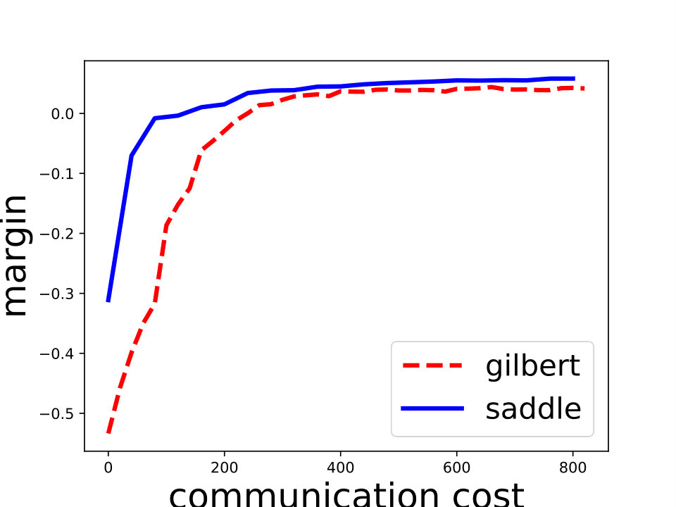 Figure 1
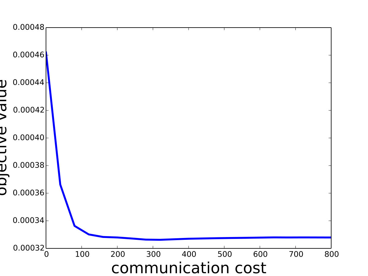 Figure 2
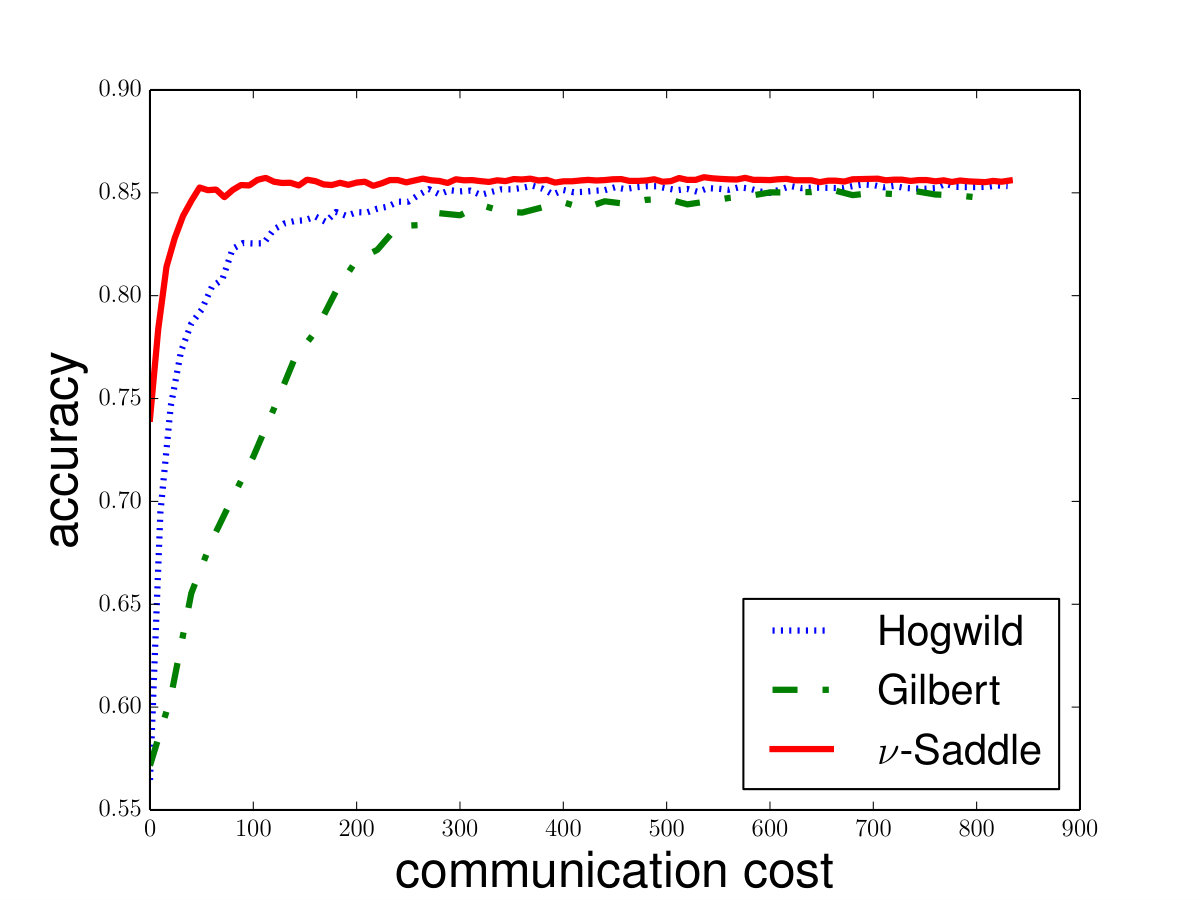 Figure 3
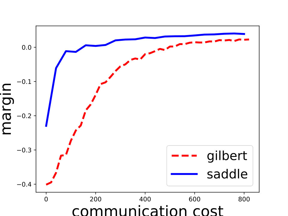 Figure 4
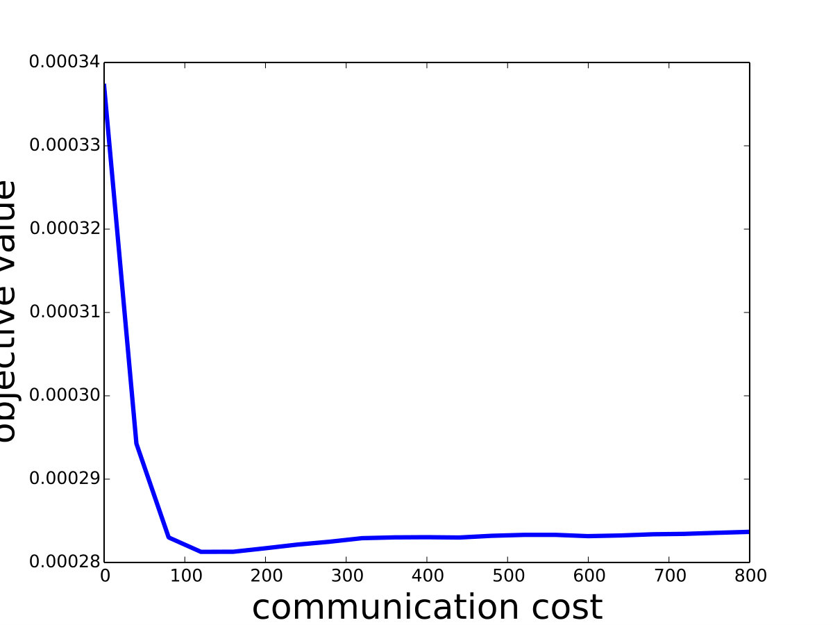 Figure 5
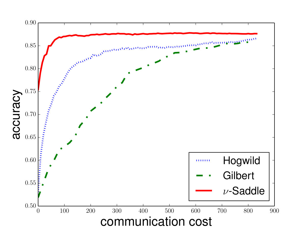 Figure 6
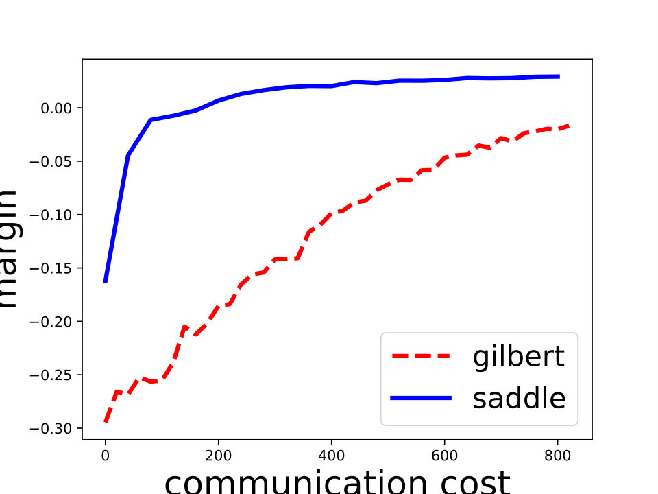 Figure 7
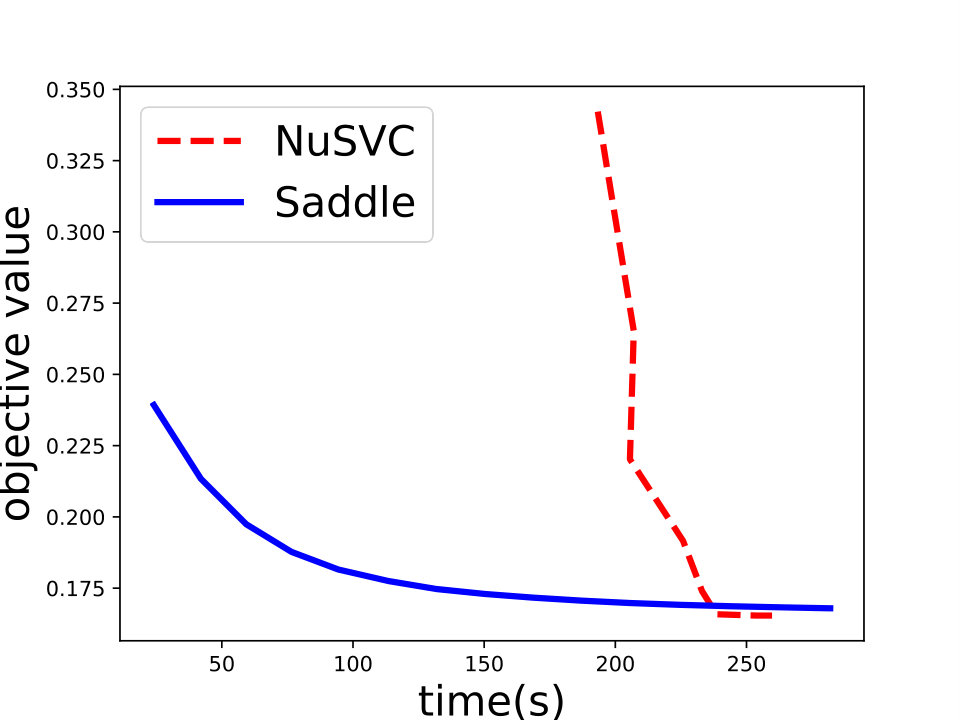 Figure 8
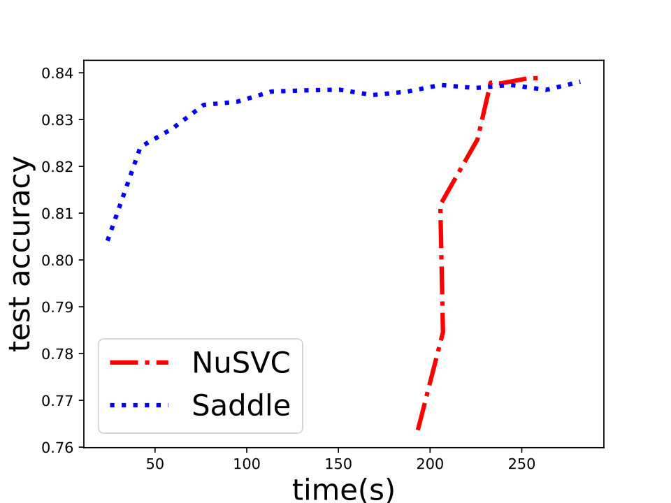 Figure 9
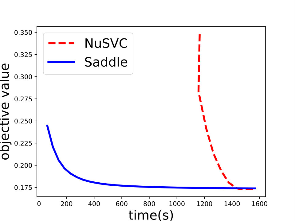 Figure 10
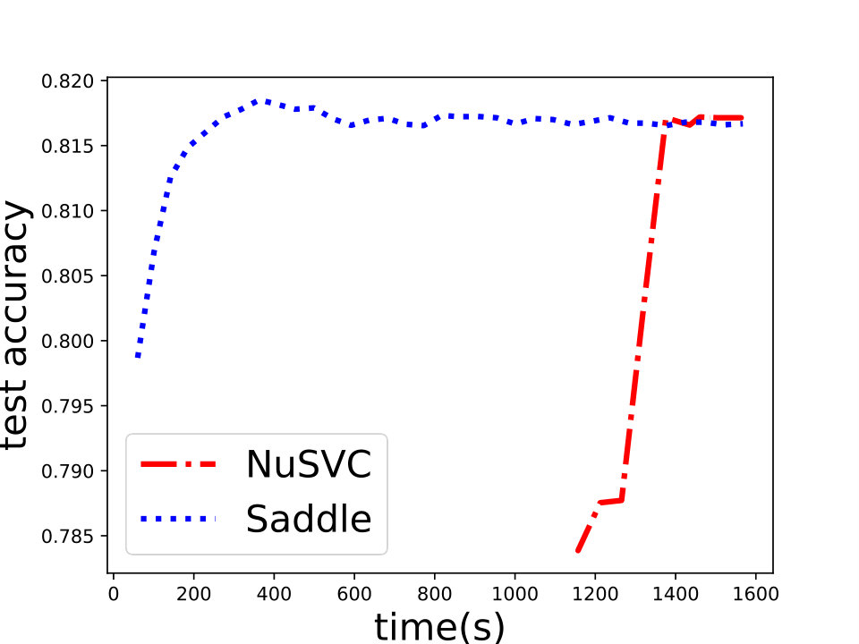 Figure 11
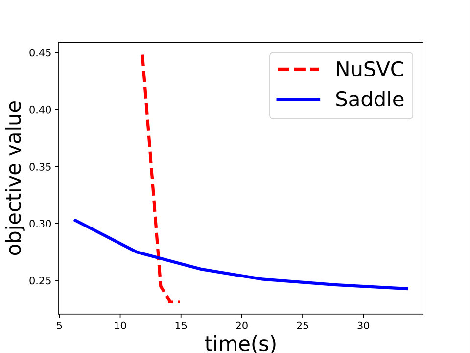 Figure 12
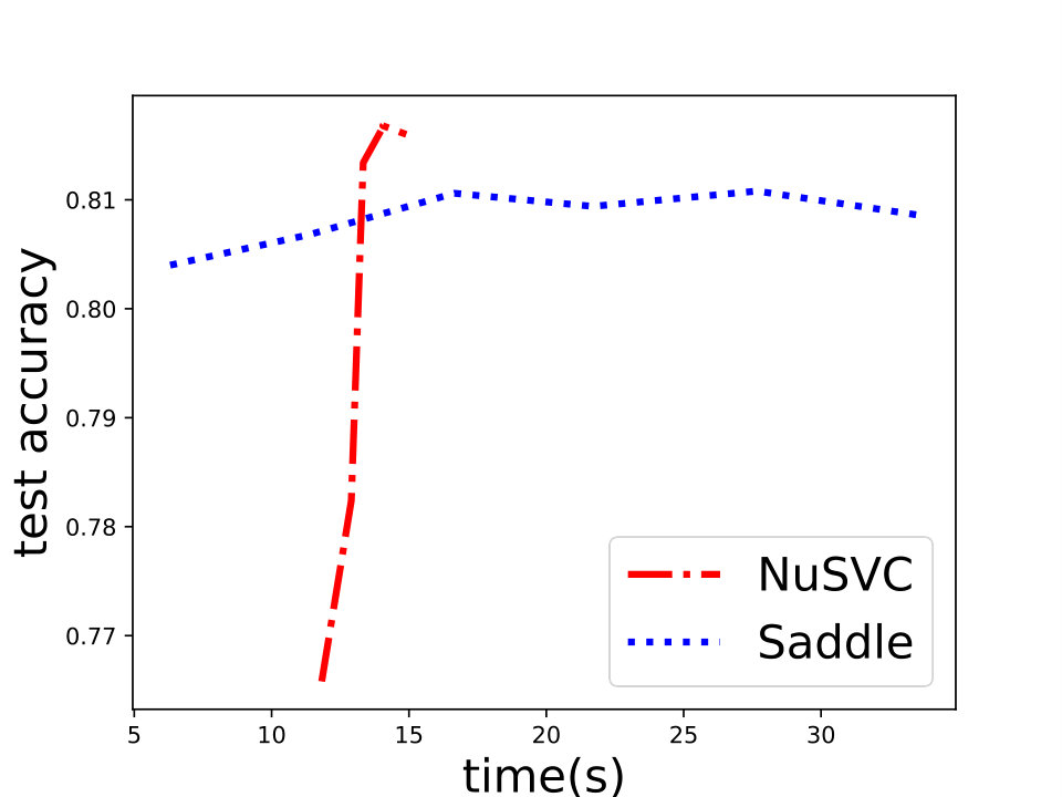 Figure 13
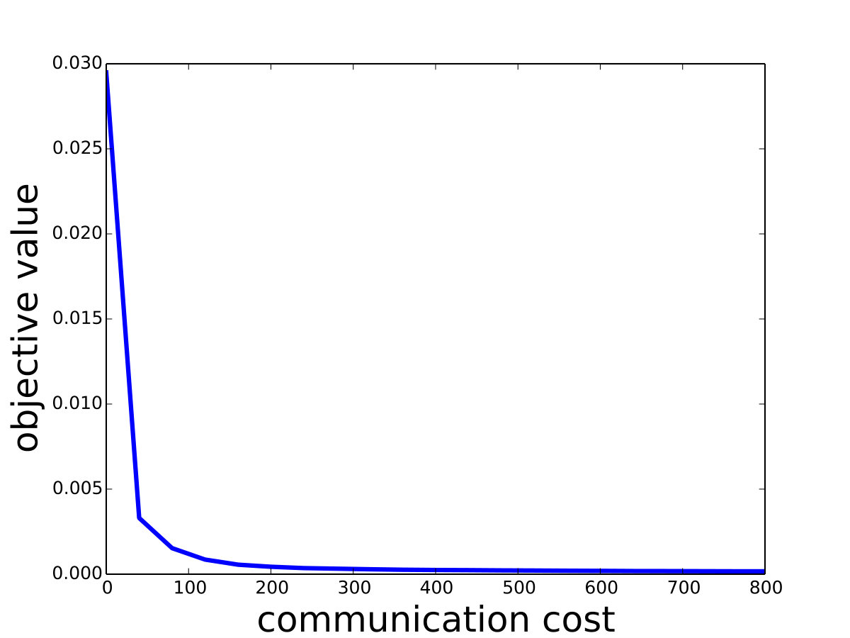 Figure 14
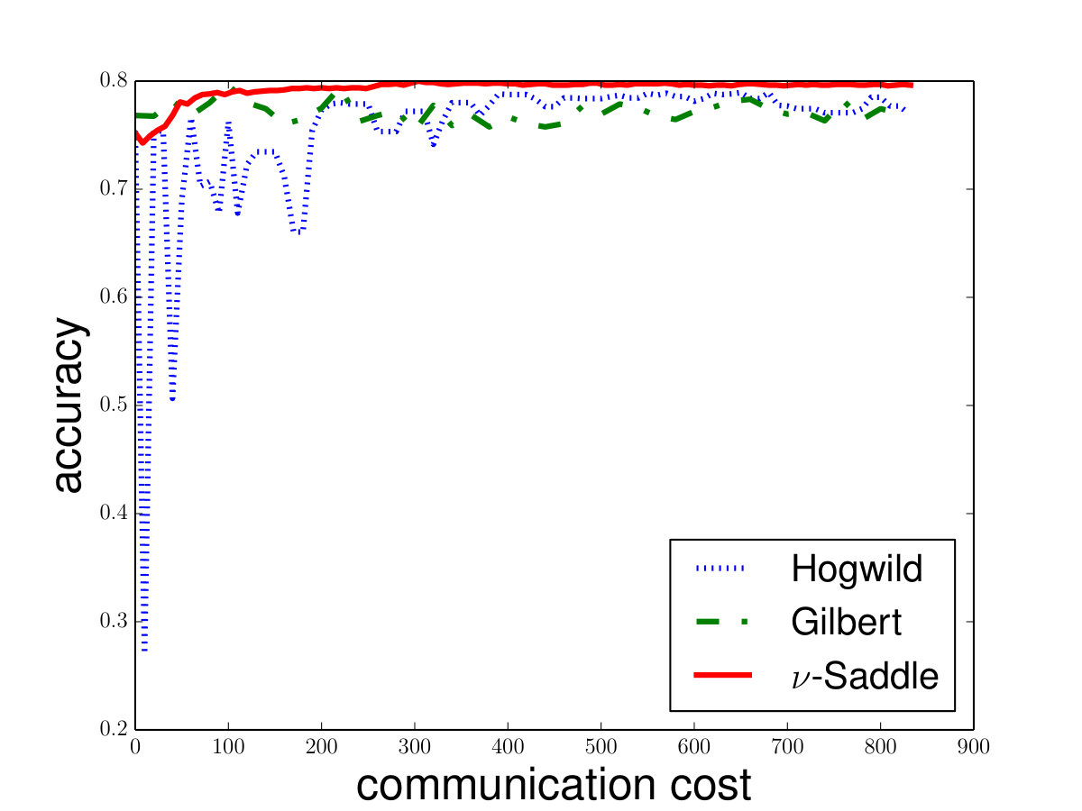 Figure 15
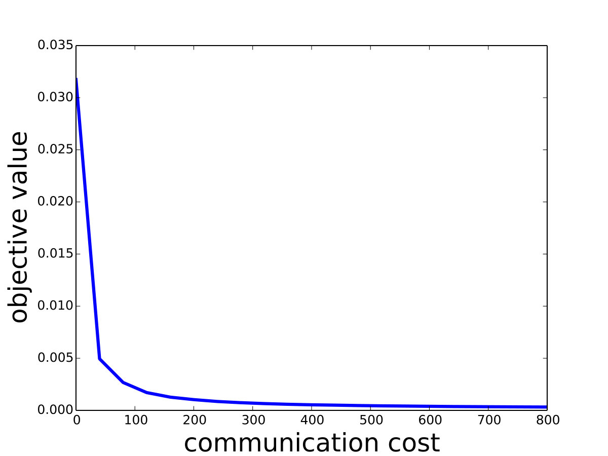 Figure 16
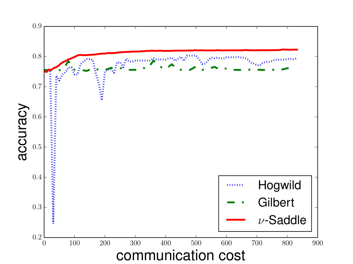 Figure 17
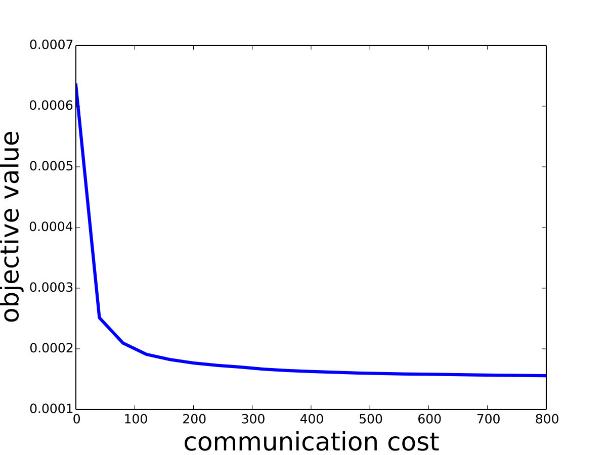 Figure 18
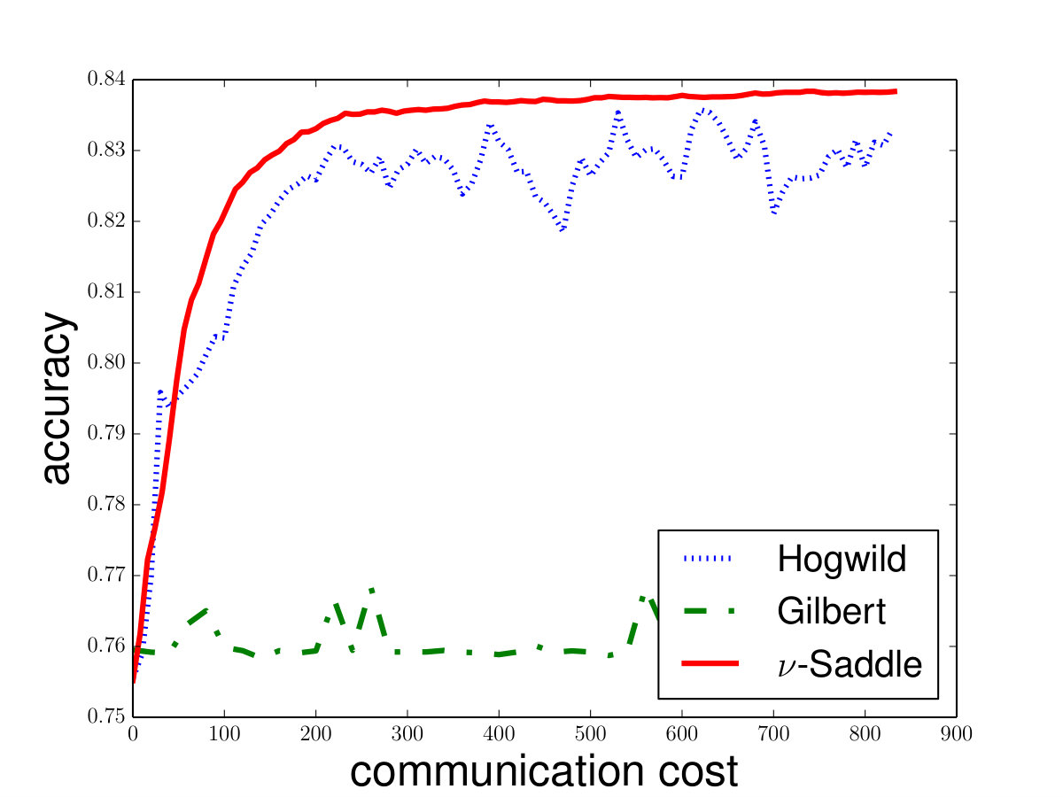 Figure 19
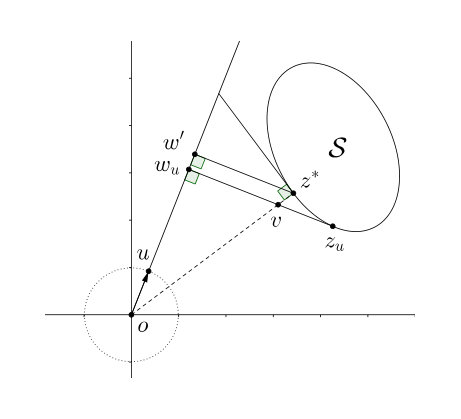 Figure 20
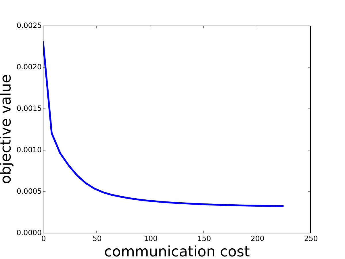 Figure 21
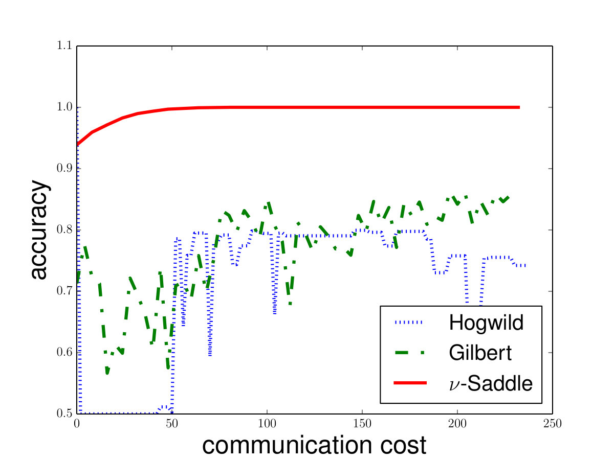 Figure 22
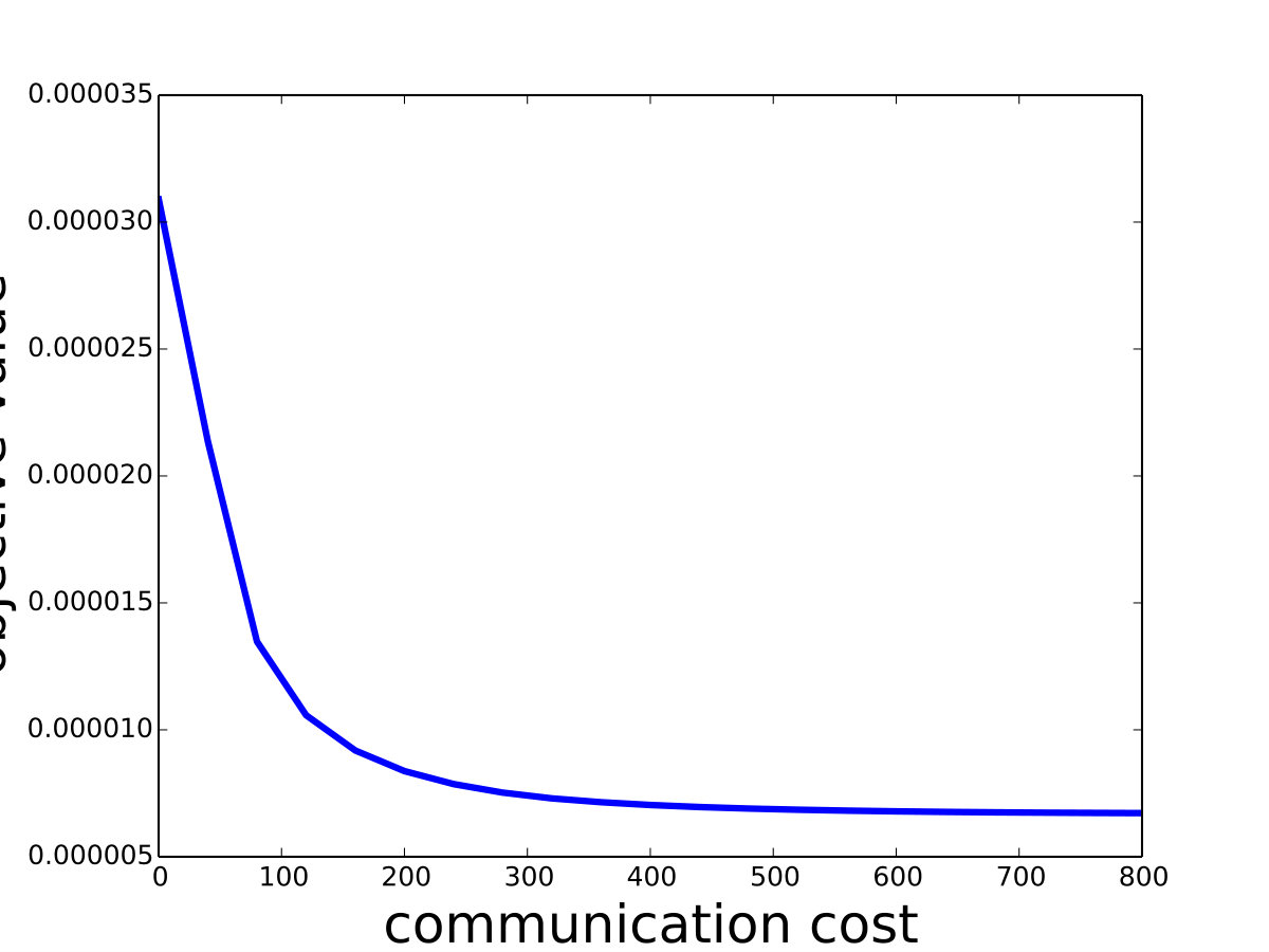 Figure 23
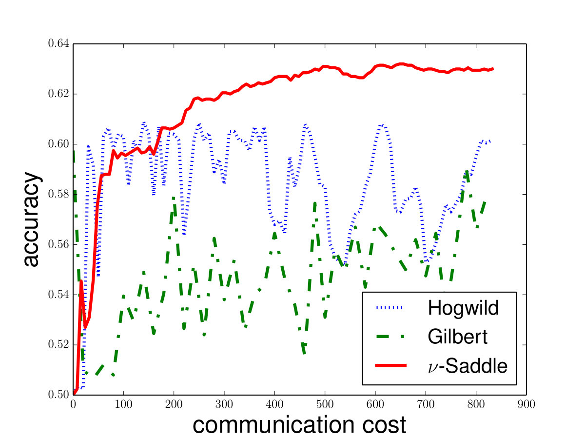 Figure 24
 Figure 25
 Figure 26
 Figure 27
 Figure 28
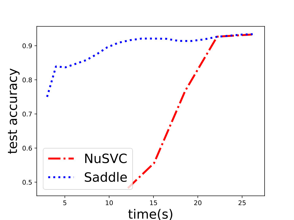 Figure 29
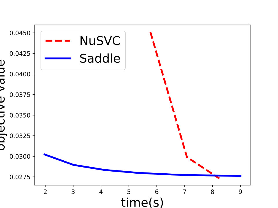 Figure 30
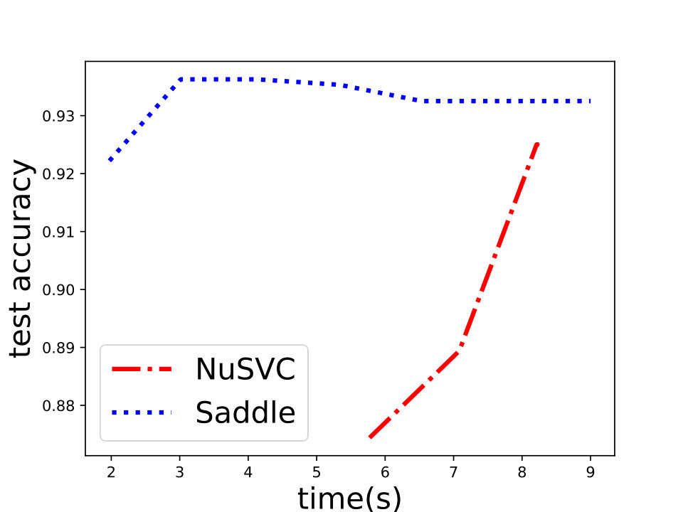 Figure 31
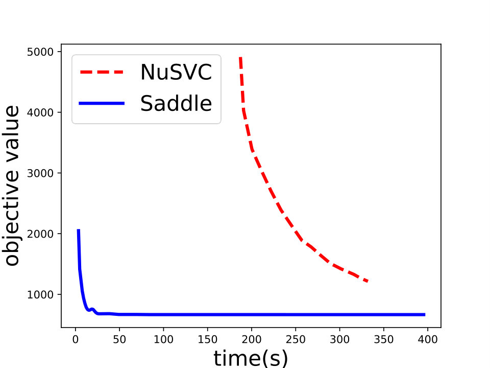 Figure 32
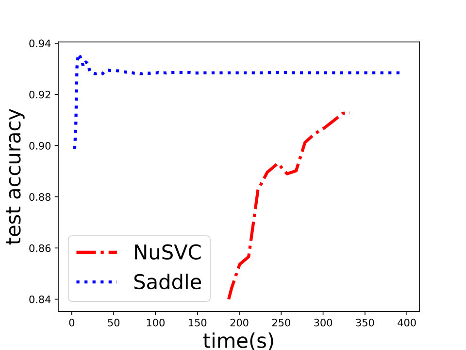 Figure 33
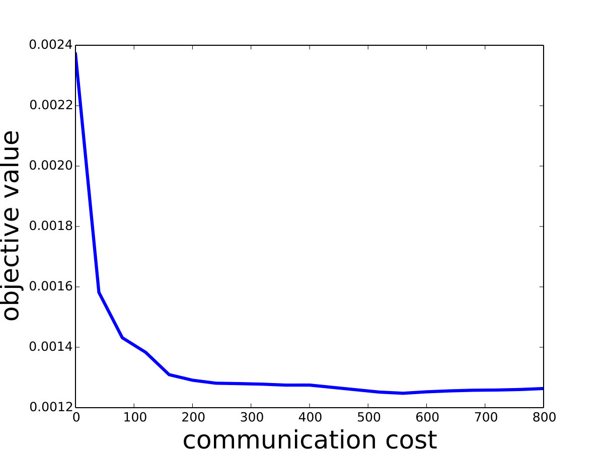 Figure 34
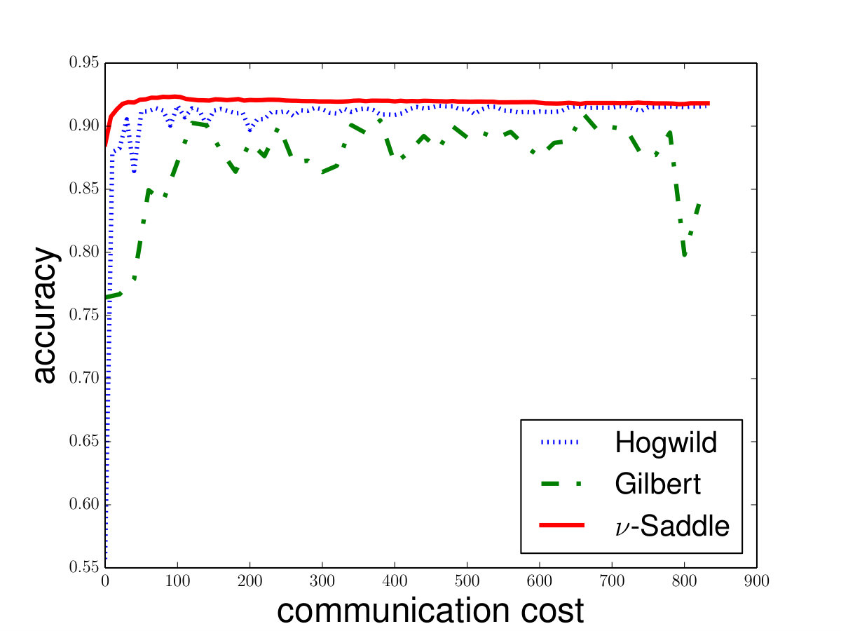 Figure 35
| data set | Saddle-SVC | Gilbert | ||
| obj | time | obj | time | |
| iris | 0.835 | 0.152s | 0.835 | 0.0005s |
| mushrooms | 0.516 | 11.2s | 0.517 | 12.5s |
| data set | parameters | ||||
| a1a | 1605 | 395 | 1210 | 119 | 0.12 |
| a5a | 6414 | 1569 | 4845 | 122 | 0.114 |
| a9a | 32561 | 7841 | 24,720 | 123 | 0.113 |
| phishing | 11055 | 6157 | 4898 | 68 | 0.441 |
| mushrooms | 8124 | 3916 | 4208 | 112 | 0.188 |
| iris | 150 | 100 | 50 | 4 | 0.978 |
| gisette | 6000 | 3000 | 3000 | 5000 | 0.99 |
| w8a | 49749 | 1479 | 48270 | 300 | 0.038 |
| ijcnn1 | 49990 | 4,853 | 45,137 | 22 | 0.590 |
| skin_nonskin | 245057 | 50859 | 194198 | 3 | 0.982 |
| data set | LIBSVM | Saddle-SVC | |||
| Obj | Test Acy | Obj | Test Acy | ||
| a9a | 0.1 | 6e-12 | 0.35 | 6e-4 | 0.69 |
| 0.3 | 6e-13 | 0.36 | 7e-4 | 0.69 | |
| 0.5 | 6e-13 | 0.71 | 3e-4 | 0.70 | |
| phishing | 0.1 | 6e-11 | 0.89 | 3e-4 | 0.82 |
| 0.3 | 0.002 | 0.93 | 0.002 | 0.93 | |
| 0.5 | 0.01 | 0.92 | 0.01 | 0.93 | |
| ijcnn1 | 0.1 | 2e-12 | 0.17 | 0.0039 | 0.73 |
| 0.3 | 6e-13 | 0.17 | 0.002 | 0.47 | |
| 0.5 | 3e-13 | 0.80 | 0.0004 | 0.31 | |
| data set | nnz | Saddle-SVC | LinearSVC | ||
| test acy | time | test acy | time | ||
| skin | 0.98 | 0.931 | 40.0s | 0.913 | 654s |
| w8a | 0.03 | 0.984 | 3075s | 0.986 | 12.5s |
| synthetic | 0.1 | 0.804 | 393s | 0.830 | 28.2s |
| synthetic | 0.5 | 0.844 | 369s | 0.843 | 214s |
| synthetic | 0.9 | 0.825 | 363s | 0.828 | 537s |
Peer Reviews
No public reviews on file for this paper yet. If you reviewed it on a platform where reviews are public (OpenReview, ICLR, NeurIPS, ICML), you can paste yours below so the community can read it here.
Videos
No videos yet. Explain this paper in a talk, walkthrough, or lecture? Add one.
Taxonomy
MethodsSupport Vector Machine
SVM via Saddle Point Optimization:
New Bounds and Distributed Algorithms
Yifei Jin
Tsinghua University
Lingxiao Huang
EPFL
Jian Li
Tsinghua University
Abstract
We study two important SVM variants: hard-margin SVM (for linearly separable cases) and -SVM (for linearly non-separable cases). We propose new algorithms from the perspective of saddle point optimization. Our algorithms achieve -approximations with running time for both variants, where is the number of points and is the dimensionality. To the best of our knowledge, the current best algorithm for -SVM is based on quadratic programming approach which requires time in worst case [23, 36]. In the paper, we provide the first nearly linear time algorithm for -SVM. The current best algorithm for hard margin SVM achieved by Gilbert algorithm [17] requires time. Our algorithm improves the running time by a factor of . Moreover, our algorithms can be implemented in the distributed settings naturally. We prove that our algorithms require communication cost, where is the number of clients, which almost matches the theoretical lower bound. Numerical experiments support our theory and show that our algorithms converge faster on high dimensional, large and dense data sets, as compared to previous methods.
1 Introduction
Support Vector Machine (SVM) is widely used for classification in numerous applications such as text categorization, image classification, and hand-written characters recognition.
In this paper, we focus on binary classification. If two classes of points which are linearly separable, one can use the hard-margin SVM ([6, 10]), which is to find a hyperplane that separate two classes of points and the margin is maximized. If the data is not linearly separable, several popular SVM variants have been proposed, such as -SVM, -SVM and -SVM (see e.g., the summary in [17]). The main difference among these variants is that they use different penalty loss functions for the misclassified points. -SVM, as the name implied, uses the penalty loss. -SVM and -SVM are two well-known SVM variants using -loss. -SVM uses the -loss with penalty coefficient [46]. On the other hand, -SVM reformulates -SVM through taking a new regularization parameter [38]. However, given a -SVM formulation, it is not easy to compute the regularization parameter and obtain an equivalent -SVM. Because the equivalence is based on some hard-to-compute constant. Compared to -SVM, the parameter in -SVM has a more clear geometric interpretation: the objective is to minimize the distance between two reduced polytopes defined based on [11]. However, the best known algorithm for -SVM is much worse than that for -SVM in practice (see below).
In general, SVMs can be formulated as convex quadratic programs and solved by quadratic programs in time [23, 36]. However, better algorithms exists for some SVM variants, which we briefly discuss below.
For hard-margin SVM, [17] showed that Gilbert algorithm [18] achieves a -approximation with running time where is the ratio of the minimum distance to the maximum one among the points. -SVM and -SVM have been studied extensively and current best algorithms runs in time linear in the number of data points [39, 15, 12, 2]. However, these techniques cannot be extended to -SVM directly, mainly because -SVM cannot be transformed to single-objective unconstrained optimization problems. Except the traditional quadratic programming approach, there is no better algorithm known with provable guarantee for -SVM. Whether -SVM can be solved in nearly linear time is still open.
Distributed SVM has also attracted significant attention in recent years. A number of distributed algorithms for SVM have been obtained in the past [19, 32, 30, 14, 44]. Typically, the communication complexity is one of the key performance measurements for distributed algorithms, and has been studied extensively (see [43, 34, 27] ). For hard-margin SVM, recently, Liu et al. [28] proposed a distributed algorithm with communication cost, where is the number of the clients. Hence, it is a natural question to ask whether the communication cost of their algorithm can be improved.
1.1 Our Contributions
We summarize our main contributions as follows.
Hard-Margin SVM: We provide a new -approximation algorithm with running time , where is the ratio of the minimum distance to the maximum one among the points (see Theorem 6). 111 notation hides logarithm factors such as , and . Compared to Gilbert algorithm [17], our algorithm improves the running time by a factor of . First, we regard hard-margin SVM as computing the polytope distance between two classes of points. Then we translate the problem to a saddle point optimization problem using the properties of the geometric structures (Lemma 2), and provide an algorithm to solve the saddle point optimization. 2. 2.
-SVM: Then, we extend our algorithm to -SVM and design an time algorithm, which is the most important technical contribution of this paper. To the best of our knowledge, it is the first nearly linear time algorithm for -SVM. It is known that -SVM is equivalent to computing the distance between two reduced polytopes [5, 11]. The obstacle for providing an efficient algorithm based on the reduced polytopes is that the number of vertices in the reduced polytopes may be exponentially large. However, in our framework, we only need to implicitly represent the reduced polytopes. We show that using the similar saddle point optimization framework, together with a new nontrivial projection method, -SVM can be solved efficiently in the same time complexity as in the hard-margin case. Compared with the QP-based algorithms in previous work [23, 36], our algorithm significantly improves the running time, by a factor of . 3. 3.
Distributed SVM: Finally, we extend our algorithms for both hard-margin SVM and -SVM to the distributed setting. We prove that the communication cost of our algorithm is , which is almost optimal according to the lower bound provided in [28]. For the hard-margin SVM, compared with the current best algorithm [28] with communication cost, our algorithm is more suitable when is small and is large. For -SVM, our algorithm is the first practical distributed algorithm.
Besides, the numerical experiments support our theoretical bounds. We compare our algorithms with Gilbert Algorithm [17] and NuSVC, LinearSVC in scikit-learn [35]. The experiments show that our algorithms converge faster on high dimensional, large and dense data sets.
1.2 Other Related Work
For the hard-margin SVM, there is an alternative to Gilbert’s method, called the MDM algorithm, originally proposed by [31]. Recently, López and Dorronsoro proved that the rate of convergence of MDM algorithm is [29] which is a linear convergence w.r.t. , but worse than Gilbert Algorithm w.r.t. .
Both -SVM and -SVM have been studied extensively in the literature. Basically, there are three main algorithmic approaches: the primal gradient-based methods [26, 39, 12, 15, 2], dual quadratic programming methods [24, 40, 22] and dual geometry methods [42, 41]. Recently, [2] provided the current best algorithms which achieve time for -SVM and time for -SVM.
Some sublinear time algorithms for hard-margin SVM and -SVM have been proposed [9, 21]. These algorithms are sublinear w.r.t. , (i.e., the size of the input), but have worse dependency on .
The algorithmic framework for saddle point optimization was first developed by Nesterov for structured nonsmooth optimization problem [33]. He only considered the full gradient in the algorithm. Recently, some studies have extended it to the stochastic gradient setting [45, 3]. The most related work is [3], in which the author obtained an algorithm for the minimum enclosing ball problem (MinEB) in Euclidean space, using the saddle point optimization. This result also implies an algorithm for -SVM, by the connection between MinEB and -SVM (see [42, 20, 41]). However, the implied algorithm is not as efficient. Based on [42, 41], the dual of -SVM is equivalent to MinEB by a specific feature mapping. It maps a -dimensional point to the -dimensional space. Thus, after the mapping, it takes quadratic time to solve -SVM. To avoid this mapping, they designed an algorithm called Core Vector Machine (CVM), in which they can solve -SVM by solving MinEB problems sequentially.
2 Formulate SVM as Saddle Point Optimization
In this section, we formulate both hard-margin SVM and -SVM, and show that they can be reduced to saddle point optimizations. All vectors in the paper are all column vectors by default.
Definition 1** (Hard-margin SVM).**
Given points for , each has a label . The hard-margin SVM can be formalized as the following quadratic programming [10].
[TABLE]
The dual problem of (1) is defined as follows, which is equivalent to finding the minimum distance between the two convex hulls of two classes of points [5] when they are linearly separable. We call the problem the C-Hull problem.
[TABLE]
where and are the matrices in which each column represents a vector of a point with label or respectively.
Denote the set of points with label by and the set with label by . Let and . Since , we can regard it as a probability distribution among points in (similarly for ). We denote to be the set of -dimensional probability vectors over and to be that over . Then, we prove that the C-Hull problem (2) is equivalent to the following saddle point optimization in Lemma 2. We defer the proof to Appendix C.
Lemma 2**.**
Problem C-Hull (2) is equivalent to the saddle point optimization (3).
[TABLE]
Let . Note that is only linear w.r.t. and . However, in order to obtain an algorithm which converges faster, we hope that the objective function is strongly convex with respect to and . For this purpose, we can add a small regularization term which ensures that the objective function is strongly convex. This is a commonly used approach in optimization (see [3] for an example). Here, we use the entropy function as the regularization term. The new saddle point optimization problem is as follows.
[TABLE]
where . The following lemma describes the efficiency of the above saddle point optimization (4). We defer the proof to Appendix C.
Lemma 3**.**
Let and be the optimal solution of saddle point optimizations (3) and (4) respectively. Define as in (3). Define
[TABLE]
Then (note that ).
We call the saddle point optimization (4) the Hard-Margin Saddle problem, abbreviated as HM-Saddle. Next, we discuss -SVM (see [11, 38]) and again provide an equivalent saddle point optimization formulation.
Definition 4** (-SVM).**
Given points for , each has a label . -SVM is the quadratic programming as follows.
[TABLE]
[11] presented a geometry interpretation for -SVM. They proved that -SVM is equivalent to the problem of finding the closest distance between two reduced convex hulls as follows.
[TABLE]
We call the above problem the Reduced Convex Hull problem, abbreviated as RC-Hull. The difference between C-Hull (2) and RC-Hull (6) is that in the latter one, each entry of and has an upper bound . Geometrically, it means to compress the convex hull of and such that the two reduced convex hulls are linearly separable. We define to be the domain of in RC-Hull, i.e., and to be the domain of , i.e., . Similar to Lemma 2, we have the following lemma. The proof is deferred to Appendix C.
Lemma 5**.**
RC-Hull (6) is equivalent to the following saddle point optimization.
[TABLE]
Again, we add two entropy terms to make the objective function strongly convex with respective to and .
[TABLE]
where . We call this problem a -Saddle problem. Similar to Lemma 3, we can prove that -Saddle (8) is a -approximation of the saddle point optimization (7). See Lemma 15 in Appendix C for the details.
Overall, we formulate hard-margin SVM and -SVM as saddle point problems and prove that through solving HM-Saddle and -Saddle, we can solve hard-margin SVM and -SVM.222 Some readers may wonder why the formulations of HM-Saddle and -Saddle only depends on but not the offset . In fact, according to the fact that the hyperplane bisects the closest points in the (reduced) convex hulls, it is not difficult to show that .
3 Saddle Point Optimization Algorithms for SVM
In this section, we propose efficient algorithms to solve the two saddle point optimizations: HM-Saddle (4) and -Saddle (8). The framework is inspired by the prior work by [3]. However, their algorithm does not imply an effective SVM algorithm directly as discussed in Section 1.2. We modify the update rules and introduce new projection methods to adjust the framework to the HM-Saddle and -Saddle problems. We highlight that both the new update rules and projection methods are non-trivial.
First, we introduce a preprocess step to make the data vectors more homogeneous in each coordinate. Then, we explain the update rules and projection methods of our algorithm: Saddle-SVC.
For convenience, we assume that in the hard margin case for . 333 It can be achieved by scaling all data by factor in time. Let be the Walsh-Hadamard matrix and be a diagonal matrix whose entries are i.i.d. chosen from with equal probability. Then, we transform the data by left-producting the matrix . Then with high probability, for any point satisfied that [1]
[TABLE]
Let and . It means that after transformation, with high probability, the value of each entry in or is at most . This transformation can be completed in time by FFT. Note that is an invertible matrix which represents a rotation and mirroring operation. Hence, it does not affect the optima of the problem. In fact, the “Hadamard transform trick” has been used in the numerical analysis literature explicitly or implicitly (see e.g., [16, 25, 3]). Roughly speaking, the main purpose of the transform is to make all coordinates of more uniform, such that the uniform sampling (line 1 in Algorithm 2) is more efficient (otherwise, the large coordinates would have a disproportionate effect on uniform sampling).
After the data transformation, we define some necessary parameters. See Line 4 of Algorithm 1 for details. 444 Careful readers may notice that . But is an unknown parameter, which is the ratio of the minimum distance to the maximum one among the points. The same issue also appears in the previous work [3]. The role of is similar to the step size in the stochastic gradient descent algorithm. In practice, we could try several for and choose the best one.
We use “” to represent the value of variable “” at iteration . For example, , are the initial value of and are defined in Line 5 of Algorithm 1.
Update Rules: In order to unify HM-Saddle and -Saddle in the same framework, we use to represent the domains in HM-Saddle (see formula (3)) or in -Saddle (see formula (7)).
Generally speaking, the update rules alternatively maximize the objective with respect to and minimize with respect to and . See the details in Algorithm 2.
Firstly, we update according to Line 4 in Algorithm 2. It is equivalent to a variant of the proximal coordinate gradient method with -norm regularization as follows.
[TABLE]
We briefly explain the intuition of (9). Note that the term in (9) can be considered as the term adding an extra momentum term and for dual variable and respectively (see Line 2 and 3 in Algorithm 2). Further, is the term in the objective function (4) and (8) which are related to . The ) is the -norm regularization term.
Moreover, rather than update the whole vector, randomly selecting one dimension and updating the corresponding in each iteration can reduce the runtime per round.
The update rules for and are listed in Line 5 and 6 in Algorithm 2, which are the proximal gradient method with a Bergman divergence regularization . Similar to in (9), we also add a momentum term for primal variable when updating and .
Projection Methods: However, the update rules for and are implicit update rules. We need to show that we can solve the corresponding optimization problems in line 5 and 6 of Algorithm 2 efficiently. In fact, for both HM-Saddle and -Saddle, we can obtain explicit expressions of these two optimization problems using the method of Lagrange multipliers.
First, we can solve the optimization problem for HM-Saddle (in Line 5 and 6) directly, and the explicit expressions for and are as follows.
[TABLE]
where and are normalizers that ensures and , and
[TABLE]
Note that the factors and are used to project the value and to the domains and . The above update rules of and can be also considered as the multiplicative weight update method (see [4]).
Next, we consider -Saddle. Compared to HM-Saddle, -Saddle has extra constraints that . Thus, we need another projection process (12) to ensure that and locate in domain and respectively. For convenience, we only present the projection for here. The projection for is similar. Let be .
[TABLE]
Note that there are at most (a constant) entries of value during the whole projection process. In each iteration, there must be at least 1 more entry since we make all entries equal to after the iteration. Thus, the number of iterations in (12) is at most . By (12), we project and to the domains and respectively.
We claim that the result of projection (12) is exactly the optimal solution in Line 5. The proof is deferred to Appendix A. Thus, we need time to compute . Since we assume that is a constant, it only costs linear time. In practice, if is extremely small, we have another update rule to get and in time. See Appendix A for details. Finally, we give our main theorem for our algorithm as follows. See the proof in Appendix C.1.
Theorem 6**.**
Algorithm 2 computes -approximate solutions for HM-Saddle and -Saddle by iterations. Moreover, it takes time for each iteration.
Combining with Lemmas 2, 3 and 5, we obtain -approximate solutions for C-Hull and RC-Hull problems. Hence by strong duality, we obtain -approximations for hard-margin SVM and -SVM in time.
Theorem 7**.**
A -approximation for either hard-margin SVM or -SVM can be computed in time.
4 Distributed SVM
Server and Clients Model: We extend Saddle-SVC to the distributed setting and call it Saddle-DSVC. We consider the popular distributed setting: the server and clients model. Denote the server by . Let be the set of clients and . We use the notation to represent any variable saved in client and use to represent a variable saved in the server.
First, we initialize some parameters in each client as the pre-processing step in Section 3. Each client maintains the same random diagonal matrix and the total number of points in each type (i.e, and ).555It can be realized using communication bits. Moreover, each client applies a Hadamard transformation to its own data and initialize the partial probability vectors and for its own points.
We first consider HM-Saddle. The interaction between clients and the server can be divided into three rounds in each iteration.
In the first round, the server randomly chooses a number and broadcasts to all clients. Each client computes and and sends them back to the server. 2. 2.
In the second round, the server sums up all and and computes and . We can see that (resp. ) is exactly (resp. ) in Algorithm 2. The server broadcasts and to all clients. By and , each client updates individually. Moreover, each client updates its own and according to the new directional vector . In order to normalize the probability vectors and , each client sends the summation and to the server. 3. 3.
In the third round, the server computes and broadcasts to all clients the normalization factors and . Finally, each client updates its partial probability vector and based on the normalization factors.
As we discuss in Section 3, for -Saddle, we need another rounds to project and to the domains and .
Each client computes and , according to (12) and sends them to the server. The server sums up all respectively and gets . If both and are zeros, the server stops this iteration. Otherwise, the server broadcasts to all clients the factors . All clients update their and according to (12) and repeat Step 4 again.
We give the pseudocode in Algorithm 4 in Appendix B. By Theorem 6, after iterations, all clients compute the same -approximate solution for SVM. W.l.o.g, let the first client send to the server. By at most more communication cost, the server can compute the offset , the margin for hard-margin SVM and the objective value for the -SVM. The correctness of Algorithm Saddle-DSVC is oblivious since we obtain the same as in Saddle-SVC after each iteration.
Communication Complexity of Saddle-DSVC: Note that in each iteration of Algorithm 4, the server and clients interact three times for hard-margin SVM and times for -SVM. Thus, the communication cost of each iteration is . By Theorem 6, it takes iterations. Thus, we have the following theorem.
Theorem 8**.**
The communication cost of Saddle-DSVC is .
Liu et el. [28] prove that the lower bound of the communication cost for distributed SVM is .
Theorem 9** (Theorem 6 in [28]).**
Consider a set of -dimension points distributed at clients. The communication cost to achieve a -approximation of the distributed SVM problem is at least for any .
If , the communication lower bound is which matches the communication cost of Saddle-DSVC.
5 Experiments
In this section, we analyze the performance of Saddle-SVC and Saddle-DSVC for both -SVM and hard-margin SVM.
First, we compare Saddle-SVC for -SVM with NuSVC in scikit-learn [35]. Current best -SVM solver is based on quadratic programming. NuSVC is one of the fastest QP-based realization, which based on the famous SVM library LIBSVM [8]. We compare Saddle-SVC with NuSVC and show that when the two reduced polytopes are linearly separable under the parameter , Saddle-SVC converges faster than NuSVC, especially when the data size is large and dense. As a supplement, in Appendix D, we also compare Saddle-SVC for -SVM with LinearSVC in scikit-learn based on LIBLINEAR [13] which is the current best algorithm for linear kernel C-SVM and -SVM.666However, we should note that LinearSVC is used to process -SVM and -loss SVM, but not -SVM or hard-margin SVM. Thus, their objective function are incomparable. We compare the test accuracy instead of the objective value. We show that for the large and dense data set, Saddle-SVC is comparable to LinearSVC and even better.
Next, we compare Saddle-SVC for hard-margin SVM with Gilbert algorithm [18]. Gilbert algorithm is the current best algorithm for hard-margin SVM. We show that Saddle-SVC converges faster when the data dimension is large.
On the other hand, we also implement our algorithm in the distributed setting and compare it with distributed Gilbert algorithm [28] and HOGWILD! [37]. We note that the current best distributed algorithm for hard-margin SVM is distributed Gilbert algorithm [28]. Our experiments indicate that Saddle-DSVC has lower communication cost in practice. On the other hand, there is no practical distributed algorithm for -SVM so far. Our algorithm is the first distributed algorithm for -SVM. To evaluate the performance of our distributed algorithm, we first show the convergence curve of Saddle-DSVC on some common datasets. As a supplement, in Appendix D, we also compare the convergent rate with HOGWILD! [37]. 777Note that HOGWILD! is used to solve -SVM or -SVM. We show that Saddle-DSVC converges faster than HOGWILD! w.r.t. communication cost.
The CPU of our platform is Intel(R) Xeon(R) CPU E5-2690 v3 @ 2.60GHz, and the system is CentOS Linux. We use both synthetic and real-world data sets. The real data sets are from [8]. See Appendix D for the way to generate synthetic data. In each experiment, we mainly care about the performance of algorithms w.r.t. and since they are data dependent parameters.
Saddle-SVC vs. NuSVC:888Note that NuSVC uses another equivalent form of -SVM. The paramater in NuSVC equals for in (5). See details in Appendix D. Here we use the data sets “a9a”, “ijcnn1”, “phishing” , and “skin_nonskin” from [8]. Note that “a9a”, “ijcnn1” has the corresponding test set “a9a.t”, “ijcnn1.t”. For “phishing” and “skin_nonskin”, we random choose data as the test set and let the remaining part be the training set. Let
[TABLE]
and set for -SVM. We show the experiment results in Figure 1 and we can see that Saddle-SVC converges faster with the similar test accuracy. Our algorithm performs much better when the data size is large. We show that the results in Figure 2 based on synthetic data sets sampling from the same distribution with different sizes.
We discuss a bit more for the parameter selection. Chang and Lin [7] show that -SVM, is feasible should larger than where and are the number of the two classes of points respectively. Moreover, if is too close to , the -SVM has poor prediction ability because of the two reduced polytopes may not separable. We discuss the detail reasons in Appendix D. We find that, in the experiment, usually ensures that the two reduced polytopes are linearly separable, i.e., the objective function converges to a positive number. In Appendix D, we also do experiments for other s and show that if is small, -SVM model has poor prediction ability.
Saddle-SVC vs. Gilbert Algorithm: For the hard-margin SVM, we compare Saddle-SVC with Gilbert Algorithm. We use linearly separable data “iris” and “mushrooms”. Since it is hard to find a large real data set which is linearly separable, we generate some synthetic data sets and show that Saddle-SVC converges faster when data dimension is large. We repeat the iterations of Saddle-SVC and compute the objective function every rounds. If the difference between two consecutive objective value is less than , then output the results. See the results in Table 1, in which we can see that Saddle-SVC gets smaller objective value (the closest distance between the two polytopes) with less running time when data dimension is large.
Saddle-DSVC: For hard-margin SVM, we compare Saddle-DSVC with distributed Gilbert algorithm. We compare the margins w.r.t. the communication cost. We count all information communication between the clients and server as the communication cost. The data sets are “mushrooms” and synthetic data sets with different dimensions. Figure 3 illustrates that Saddle-DSVC converges faster w.r.t. communication cost. The data is distributed to nodes. Note that it takes communication cost if each client sends a point to the server. We set one unit of -coordinate to represent communication cost.
For the -SVM, we analyze the convergence property on some common data sets including “phishing”, “a9a”, “gisette”, “madelon” from [8]. We show the details in Figure 4. Besides, we also compare Saddle-DSVC with HOGWILD!. We compare the accuracy instead of objective value since they solve different SVM variants. We provide the experiment details in Appendix D and show that our algorithm is convergent faster w.r.t. communication cost.
Appendix A The Equivalence of the Explicit and Implicit Update Rules of and
Lemma 10** (Update Rules of HM-Saddle).**
The following two update rules are equivalent.
- •
**
[TABLE]
- •
**
[TABLE]
for each , where 999Recall that is the th column of .
Proof.
The Lagrangian function of the first optimization formulation is
[TABLE]
Thus, we have
[TABLE]
Solve the above equalities, we obtain
[TABLE]
∎
Lemma 11** (Update Rules of -Saddle).**
The following three update rules are equivalent.
Rule 1:* *
[TABLE]
Rule 2:**
- •
Step 1:
[TABLE]
for each , where .
- •
Step 2: Sort by the increasing order. W.l.o.g., assume that is in increasing order. Define and . Find the largest index such that and by binary search.
- •
Step 3:
[TABLE]
Rule 3:**
- •
Step 1:
[TABLE]
for each , where .
- •
Step 2:
[TABLE]
Proof.
Similar to the proof of Lemma 10, we first give the Lagrangian function of the first optimization formulation as follows.
[TABLE]
By KKT conditions, we have the following.
[TABLE]
We first show the equivalence between Rule 1 and Rule 2. Note that in Rule 2 satisfies the second and the fourth KKT conditions. We only need to give all and satisfying other KKT conditions for Rule 2. Let
[TABLE]
Let
[TABLE]
as defined in Step 1 of Rule 2. For , let . For , let
[TABLE]
The inequality follows from the definition of . Note that we only need to prove that . If , then the above inequality holds directly. Otherwise if and , we have that and . We also have the following inequality
[TABLE]
which contradicts with the definition of . Finally, randomly choose an index , let
[TABLE]
By the chosen of , it is not hard to check that the value of is the same for any index . Thus, and are the unique solution of KKT conditions. So Rule 1 and Rule 2 are equivalent. By a similar argument (define suitable and ), we can prove that Rule 1 and Rule 3 are equivalent, which finishes the proof. ∎
Remark 12**.**
We analyze Rule 2 in Lemma 11. Roughly speaking, we find a suitable value , set all value to be , and scales up other values by some factor . We can verify that the running time of Rule 2 is since both the sorting time and the binary search time are . On the other hand, recall that the running time of Rule 3 is (explained in Section 3). Thus, if the parameter is extremely small, we can use Rule 2 in practice.
Appendix B Details for Distributed Algorithms: Saddle-DSVC
This section is supplementary for Section 4. First, we give the pseudocode of DisSaddle-SVC. See Algorithm 3 for the pre-processing step for each clients. Recall that we assume there are points and points maintained in . We use to denote a vector with all components being . The initialization is as follows.
[TABLE]
Next, see Algorithm 4 for the interactions between the server and clients in every iteration. Note that only -Saddle needs the fourth round in Algorithm 4. We use to distinguish the two cases. If we consider -Saddle, let be True. Otherwise, let be False.
Then, we analyze the communication cost.
Theorem 13**.**
The communication cost of Saddle-DSVC is .
Proof.
Note that in each iteration of Algorithm 4, the server and clients interact three times for hard-margin SVM and times for -SVM. The communication cost of each iteration is . By Theorem 6, it takes iterations. Thus, the total communication cost is . ∎
1: for to do
2: # first round
3: Server: Pick an index uniformly at random and send to every client.
4: for client do
5:
6:
7: Send and to server.
8: end for
9: # second round
10: Server: Let and . Broadcast and .
11: for client do
12: \left\{\begin{array}[]{ll}(w_{i}[t]+\sigma(S.\delta_{i}^{+}-S.\delta_{i}^{-}))/(\sigma+1),&\text{if }i=i^{*}\\ x\end{array}\right.
13: \exp\big{\{}(\gamma+d\tau^{-1})^{-1}(d\tau^{-1}\log C.\eta_{j}[t] \hskip 113.81102pt-\langle w[t]+d(w[t+1]-w[t]),C.X^{+}_{\cdot j}\rangle)\big{\}}
14: \exp\big{\{}(\gamma+d\tau^{-1})^{-1}(d\tau^{-1}\log C.\xi_{j}[t] \hskip 113.81102pt+\langle w[t]+d(w[t+1]-w[t]),C.X^{-}_{\cdot j}\rangle)\big{\}}
15:
16: Send and to server
17: end for
18: # third round
19: Server: Let , and broadcast and .
20: for client do
21: ,
22: end for
23: # fourth round, only for -Saddle. is true if use the code for -Saddle
24: if ** is True** then
25: repeat
26: for client do
27: , .
28: , .
29: Send to server.
30: end for
31: Server: .
32: for client do
33: , ; ,
34: , ; ,
35: end for
36: until and are zeroes
37: end if
38: end for
Liu et al. [28] proved a theoretical lower bound of the communication cost for distributed SVM as follows. Note that the statement of Theorem 14 is not exactly the same as the Theorem 6 in [28]. This is because they omit the case that . We prove that they are equivalent briefly. Note that if , the communication lower bound is which matches the communication cost of our algorithm Saddle-DSVC.
Theorem 14** (Theorem 6 in [28]).**
Consider a set of -dimension points distributed at clients. The communication cost to achieve a -approximation of the distributed SVM problem is at least for any .
Proof Sketch.
In Theorem 6 of [28], the authors obtain a lower bound if . Their proof can be extended to the case . In this case, we can make a reduction from the -OR problem in which each client maintains a -bit vector instead of a -bit vector. As the proof of Theorem 6 in [28], we can obtain a lower bound , which proves the theorem. ∎
Appendix C Missing Proofs
Lemma 2 **** (restated).
Problem C-Hull (2) is equivalent to the saddle point optimization (3).
Proof.
Consider the saddle point optimization (3). First, note that
[TABLE]
The range of the term for is a convex set, denoted by . Since the convex hulls of and are linearly separable, we have . Denote for any . Then (3) is equivalent to . Note that
[TABLE]
Thus, we only need to consider those directions such that there exists a point with . We use to denote the collection of such directions.
Let be a unit vector in . Denote
[TABLE]
By this definition, is the point with smallest projection distance to among (see Figure 5). Observe that if a direction (), then we have . Also note that
[TABLE]
Let
[TABLE]
is the projection point of to the line , where is the origin. See Figure 5 for an example. Overall, we have
[TABLE]
The last equality is by the Pythagorean theorem. Let be the closest point in to the origin point. Next, we show that . Given a unit vector , define to be the projection point of to the line . By the definition of and , we have that . Moreover, let . In this case, we have . Thus, we conclude that .
Overall, we prove that
[TABLE]
Thus, C-Hull (2) is equivalent to the saddle point optimization (3). ∎
Lemma 3 **** (restated).
Let and be the optimal solution of saddle point optimizations (3) and (4) respectively. Define as in (3). Define
[TABLE]
Then (note that ).
Proof.
Let
[TABLE]
By the definition of saddle points, we have
[TABLE]
Note that entropy function satisfies for any . Thus, . Overall, we prove that . ∎
Lemma 5 **** (restated).
RC-Hull (6) is equivalent to the following saddle point optimization.
[TABLE]
Proof.
The proof is almost the same to the proof of Lemma 2. The only difference is that the range of the term is another convex set defined by . ∎
Lemma 15**.**
Let and be the optimal solution of saddle point optimizations (7) and (8) respectively. Define as in (7). Define
[TABLE]
Then .
Proof.
Note that is a convex polytope contained in and is a convex polytope contained in . It is not hard to verify that the proof of Lemma 3 still holds for and . ∎
C.1 Proof of Theorem 6
For preparation, we give two useful Lemmas 16 and 17. Recall that is the Bregman divergence function which is defined as .
The two lemmas generalize Lemma A.1 and Lemma A.2 in [3] by changing the domain to a convex polytope contained in . However, refer to the proofs of Lemma A.1 and Lemma A.2, it still work for the general version.
Lemma 16**.**
Let . Let be a convex polytope contained in . Then for every , we have
[TABLE]
Lemma 17**.**
Let . Let be a convex polytope contained in . Then for all ,
[TABLE]
Combing the above lemmas and almost the same analysis as in Theorem 2.2 in [3], we obtain the following Theorem 18.
Theorem 18**.**
After iterations of Algorithm 2 (both HM-Saddle and -Saddle versions), we obtain a directional vector satisfying that
[TABLE]
where , for some
Proof Sketch.
The difference between our statement and Theorem 2.2 in [3] is that we update two probability vectors and instead of one in an iteration. Thus, we have two terms and on the left hand side. Moreover, we care about convex polytopes and instead of and .
However, these differences do not influence the correctness of the proof of Theorem 2.2 in [3]. Note that we replace Lemma A.1 and Lemma A.2 in [3] by Lemma 16 and Lemma 17. It is not hard to verify the proof of Theorem 2.2 in [3] works for our theorem. ∎
We also need the following lemma.
Lemma 19**.**
Define
[TABLE]
where and are two convex polytopes such that and . For any , we have
[TABLE]
Proof.
Denote by any subgradient of at point . We write for any arbitrary satisfying that . Note that (resp. ) can be considered as a weighted combination of all points (resp. ), we claim that () owing to the assumption that every satisfies . Next, we compute as follows
[TABLE]
∎
Now we are ready to prove Theorem 6 as follows.
Theorem 6 **** (restated).
Algorithm 2 computes -approximate solutions for HM-Saddle and -Saddle by iterations. Moreover, it takes time for each iteration.
Proof.
Let
[TABLE]
According to Theorem 18, we have
[TABLE]
In order to get a -approximate solution, according to Lemma 19, it suffices to choose such that
[TABLE]
Note that . Thus, we only need to have
[TABLE]
∎
Appendix D Supplementary Materials of Experiments
Data set: We use both synthetic and real-world data sets. The real data is from [8] including the separable data set “iris” and “mushrooms” and non-separable data set “w8a”, “gisette”, “madelon”, “phishing”, “a1a”, “a5a”,“a9a”, “ijcnn1”, “skin_nonskin”. We summary the information of the data in Table 2.
Besides the real world data, we generate some synthetic data sets. There are three types synthetic data: 1) separable synthetic data, 2) non-separable synthetic data, 3) sparse non-separable synthetic data. We describe the ways to generate them as follows.
- •
Separable synthetic data: we randomly choose a hyperplane which overlaps with the unit norm ball in space. Then we randomly sample points in a subset of the unit ball such that the ratio of the maximum distance among the points to over the minimum distance to is . Let the labels of points above be and let others be .
- •
Non-separable synthetic data: The difference from the separable synthetic data is that for those points with distance to smaller than , we randomly choose their labels to be or with equal probability. Moreover, we also use real-world
- •
Sparse non-separable synthetic data: First, we set a parameter “nnz” which represent the number of non-zeros elements in each point. The only difference between the dense non-separable synthetic data is that we randomly sample points such that each point only has “nnz” non-zeros non-zeros points.
-SVM form used in NuSVC: The form of the -SVM used in scikit-learn is a variant of the form in the paper. We give the formulation as follows.
[TABLE]
[11] prove that through reparameterizing, the above formulation is equivalent to -SVM (5). Concretely speaking, let
[TABLE]
Then, (14) can be transformed to -SVM (5).
Parameter in -SVM: As we have discussed in Section 5, although when belongs to , -SVM has feasible solution, where is the number of points with positive label and is the number of points with negative label. Not all feasible can induce a reasonable prediction model. If is too close to 1, the two reduced polytopes are not separable. The closest distance between the two reduced polytopes is zero. Note that in general the overlapping points are not unique. Hence the solution is not unique. Moreover, because the solution corresponds two overlapped points, the vector (which represents the vector determined by the two points) is not unique, hence, is unstable. Overall, here we select a relatively small .
Recall that we let
[TABLE]
We set and train the -SVM model on the data set “a9a”, “ijcnn1”, “phishing”. We list the results in Table 3.
Saddle-SVC vs. LinearSVC: As discussed before, they solve different SVM variants. Thus, we use the test accuracy instead of the objective values to evaluate the convergent rate. First, we explain the stop criteria of Saddle-SVC. In Theorem 7, we prove that Saddle-SVC converge in rounds. Let . We repeat the iterations of Saddle-SVC and compute the objective function every rounds. If the difference between two consecutive objective value is less than , then output the results. We note that LinearSVC is very efficient for sparse data set. But for the dense data set, Saddle-SVC performs better. In the experiment, we use “nnz” to represent the ratio of non-zero elements to all elements. We show that the parameter nnz significant affects the efficient of LinearSVC, but Saddle-SVC is barely affected. We use “skin_nonskin” and “w8a” and synthetic data sets with different parameter nnz to evaluate the performance. We list the details in Table 4.
Saddle-DSVC vs. HOGWILD!: As Saddle-DSVC is the first practical distributed algorithm for -SVM. We use another popular distributed algorithm called HOGWILD! for comparison. Note that HOGWILD! is use to solve -SVM and -SVM but not, -SVM. Thus, instead of the objective function, we use the accuracy to evaluate the performance of the algorithms. Here we choose use HOGWILD! for -SVM and Saddle-DSVC for -SVM. See the details in Figure 6. For comparison, we also provide the results of Gilbert Algorithm. Here we choose for Saddle-DSVC and for HOGWILD!. We can see that Saddle-DSVC converges faster than HOGWILD! w.r.t. communication cost. Moreover, Saddle-DSVC is more stable than HOGWILD! algorithm.
The reference list from the paper itself. Each links out to its DOI / PubMed record.
- 1[1] Nir Ailon and Bernard Chazelle. Faster dimension reduction. Communications of the ACM , 53(2):97–104, 2010.
- 2[2] Zeyuan Allen-Zhu. Katyusha: The first direct acceleration of stochastic gradient methods. STOC 16 , 2016.
- 3[3] Zeyuan Allen-Zhu, Zhenyu Liao, and Yang Yuan. Optimization algorithms for faster computational geometry. In LIP Ics , volume 55, 2016.
- 4[4] Sanjeev Arora, Elad Hazan, and Satyen Kale. The multiplicative weights update method: a meta-algorithm and applications. Theory of Computing , 8(1):121–164, 2012.
- 5[5] Kristin P Bennett and Erin J Bredensteiner. Duality and geometry in svm classifiers. In ICML , pages 57–64, 2000.
- 6[6] Bernhard E Boser, Isabelle M Guyon, and Vladimir N Vapnik. A training algorithm for optimal margin classifiers. In Proceedings of the fifth annual workshop on Computational learning theory , pages 144–152. ACM, 1992.
- 7[7] Chih-Chung Chang and Chih-Jen Lin. Training v-support vector classifiers: theory and algorithms. Neural computation , 13(9):2119–2147, 2001.
- 8[8] Chih-Chung Chang and Chih-Jen Lin. Libsvm: a library for support vector machines. TIST , 2(3):27, 2011.