Survey of Water and Ammonia in Nearby galaxies (SWAN): Resolved Ammonia Thermometry, Water and Methanol Masers in the Nuclear Starburst of NGC 253
Mark Gorski, J\"urgen Ott, Richard Rand, David S. Meier, Emmanuel, Momjian, Eva Schinnerer

TL;DR
This paper presents a detailed molecular line survey of NGC 253, revealing the physical conditions of star-forming gas, including temperature, maser activity, and possible heating mechanisms, using VLA observations across multiple molecular transitions.
Contribution
It provides the first comprehensive analysis of ammonia, water, and methanol masers in NGC 253, offering insights into the heating processes and gas dynamics in a starburst galaxy.
Findings
Molecular gas exhibits two kinetic temperature components at 130K and 57K.
Evidence suggests turbulence or cosmic rays, not photon-dominated regions or shocks, heat the gas.
Detection of ammonia and water masers indicates active star formation and complex gas motions.
Abstract
We present Karl G Jansky Very Large Array molecular line observations of the nearby starburst galaxy NGC 253, from SWAN: "Survey of Water and Ammonia in Nearby galaxies". SWAN is a molecular line survey at centimeter wavelengths designed to reveal the physical conditions of star forming gas over a range of star forming galaxies. NGC 253 has been observed in four 1GHz bands from 21 to 36 GHz at 6" (pc) spatial and 3.5 km s spectral resolution. In total we detect 19 transitions from seven molecular and atomic species. We have targeted the metastable inversion transitions of ammonia (NH) from (1,1) to (5,5) and the (9,9) line, the 22.2 GHz water (HO) () maser, and the 36.1 GHz methanol (CHOH) () maser. Utilizing NH as a thermometer, we present evidence for uniform heating over the central kpc of NGC 253. The molecular gas is…
Click any figure to enlarge with its caption.
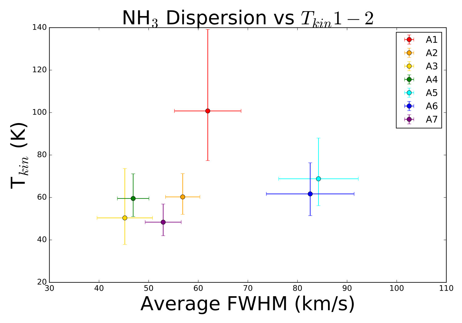 Figure 1
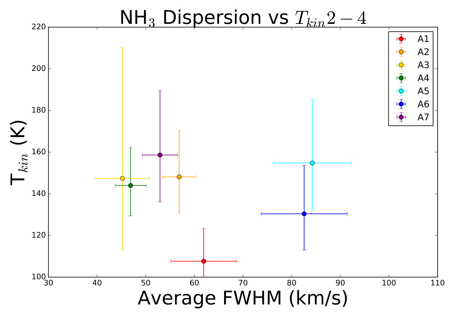 Figure 2
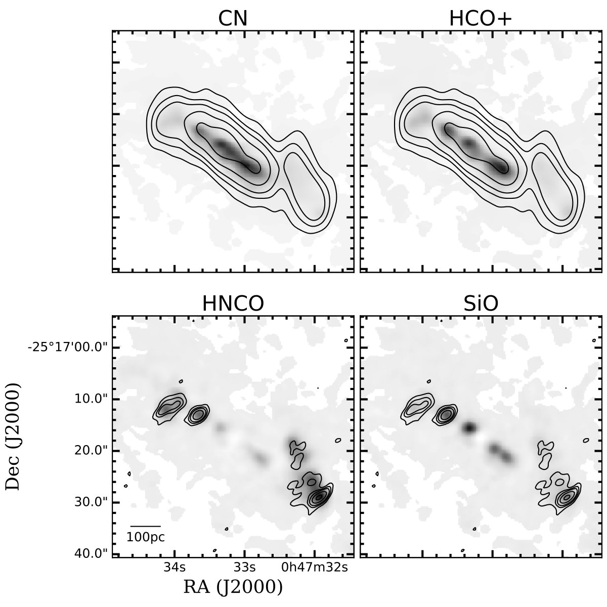 Figure 3
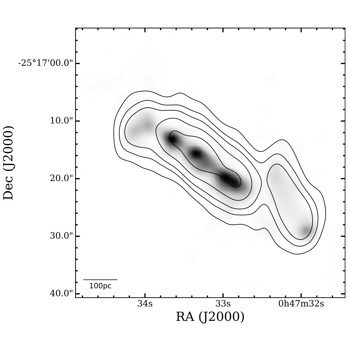 Figure 4
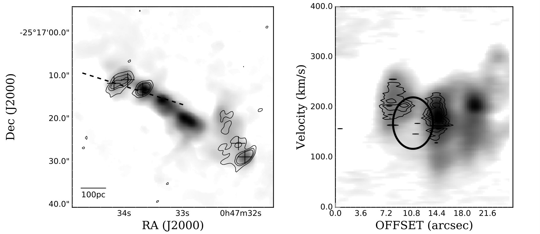 Figure 5
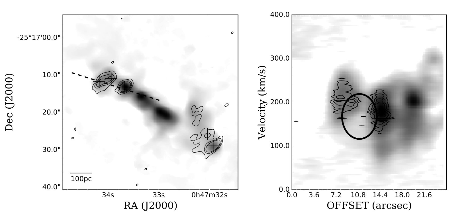 Figure 6
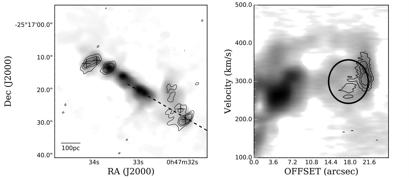 Figure 7
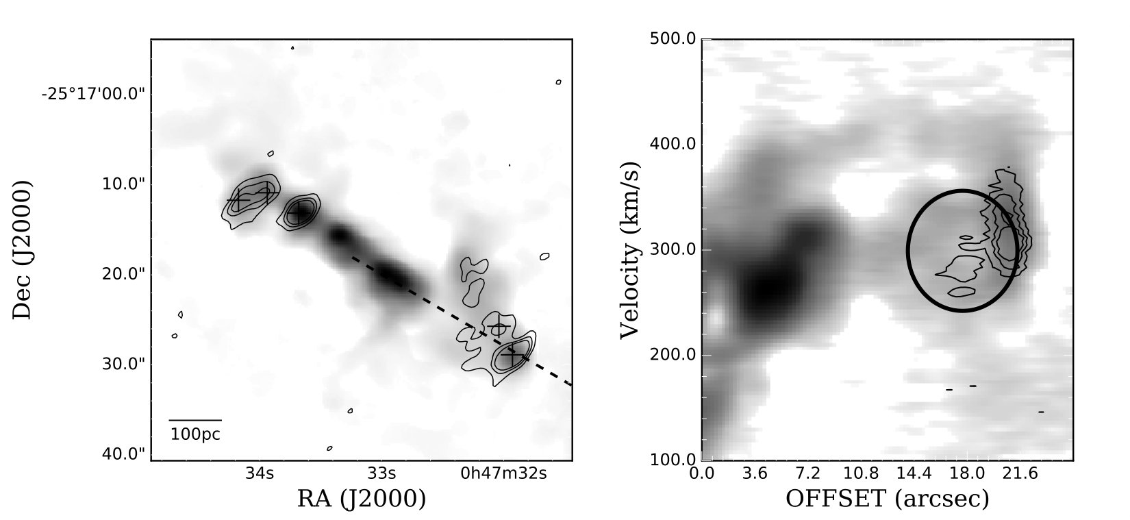 Figure 8
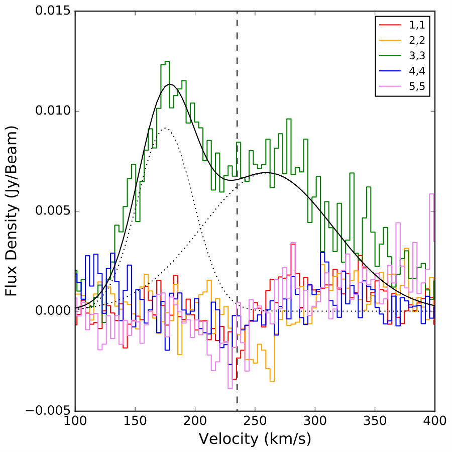 Figure 9
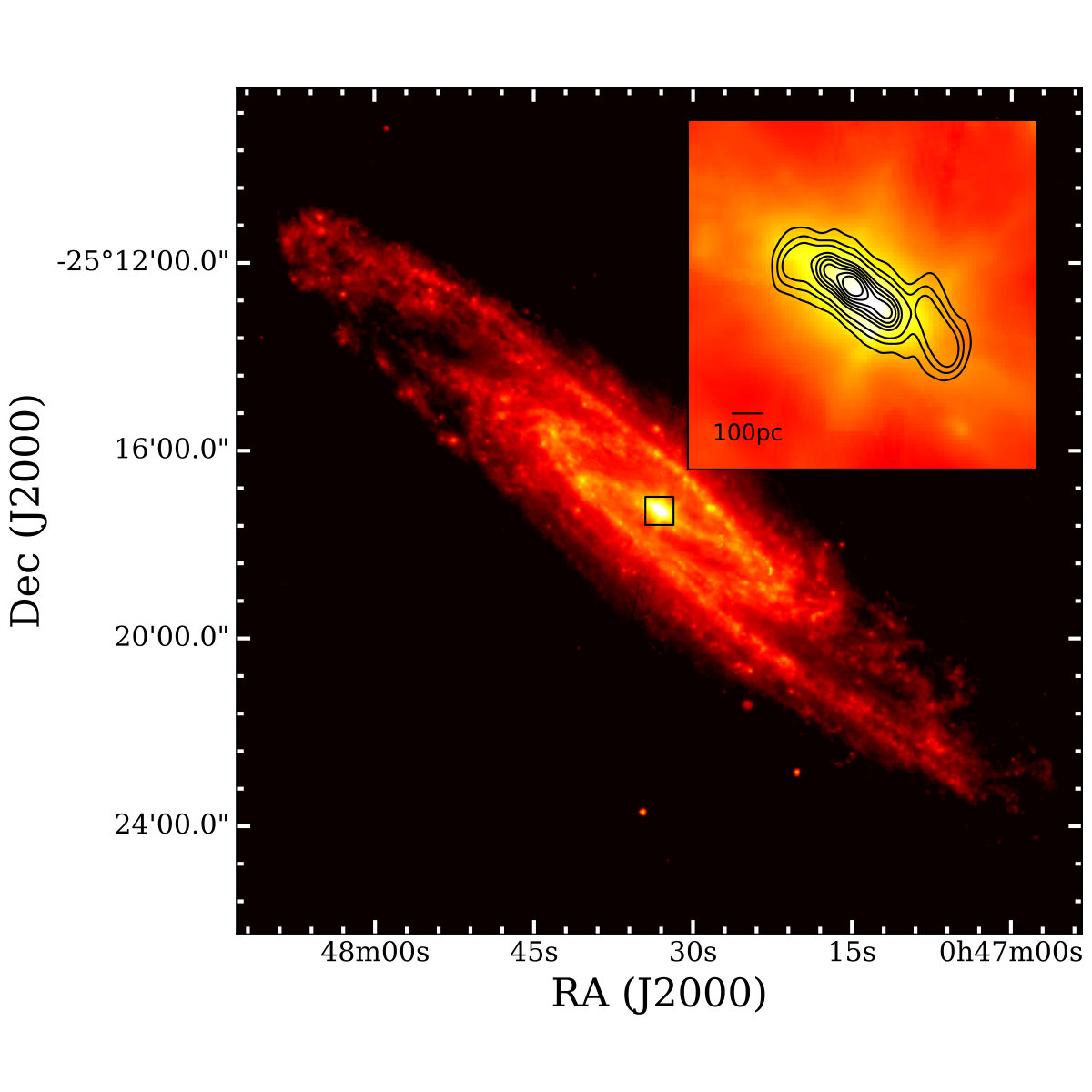 Figure 10
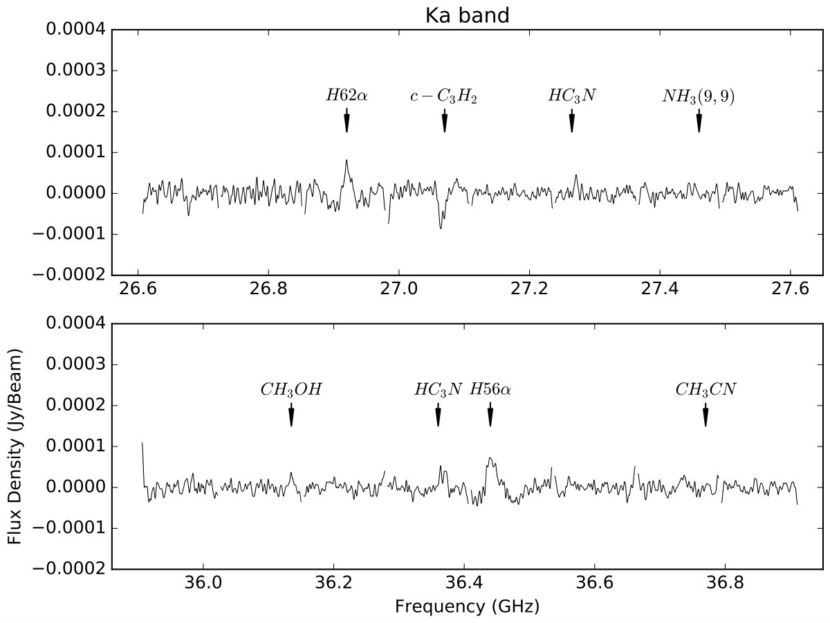 Figure 11
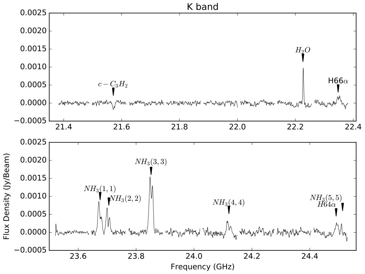 Figure 12
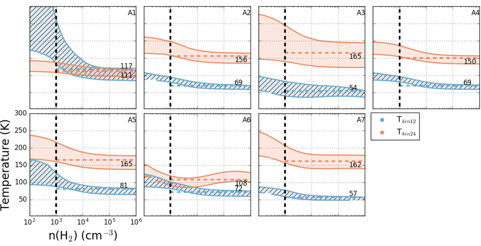 Figure 13
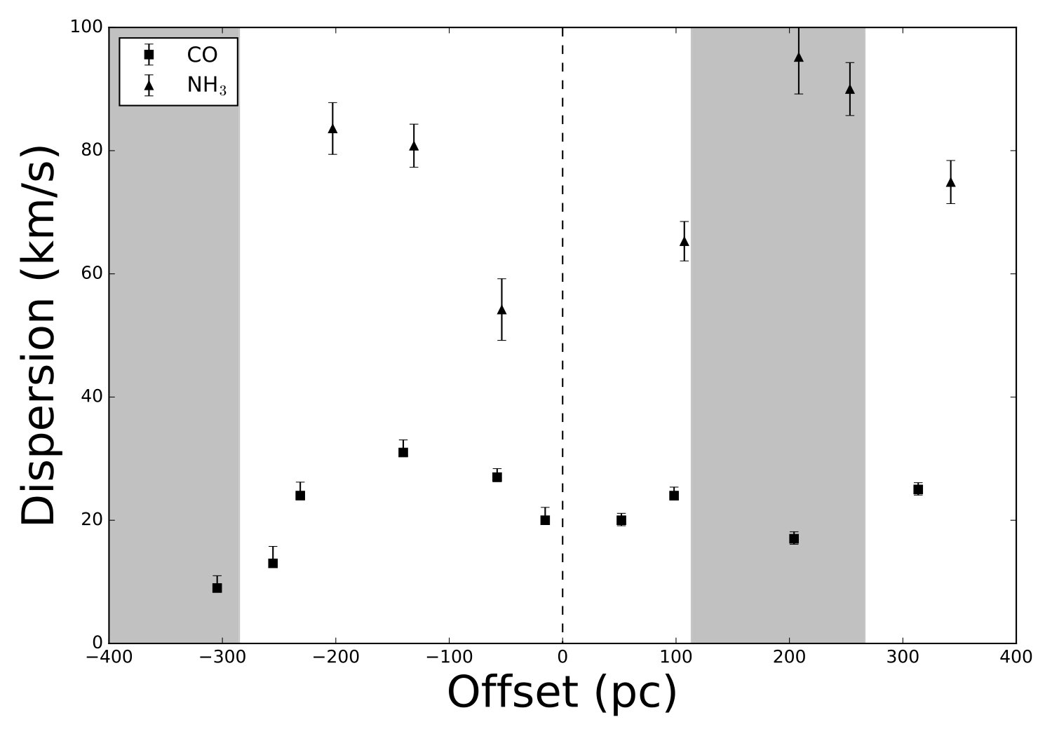 Figure 14
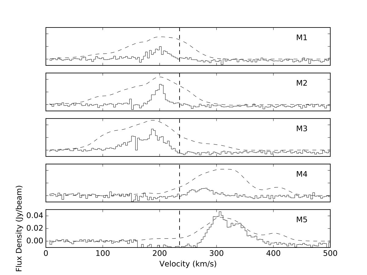 Figure 15
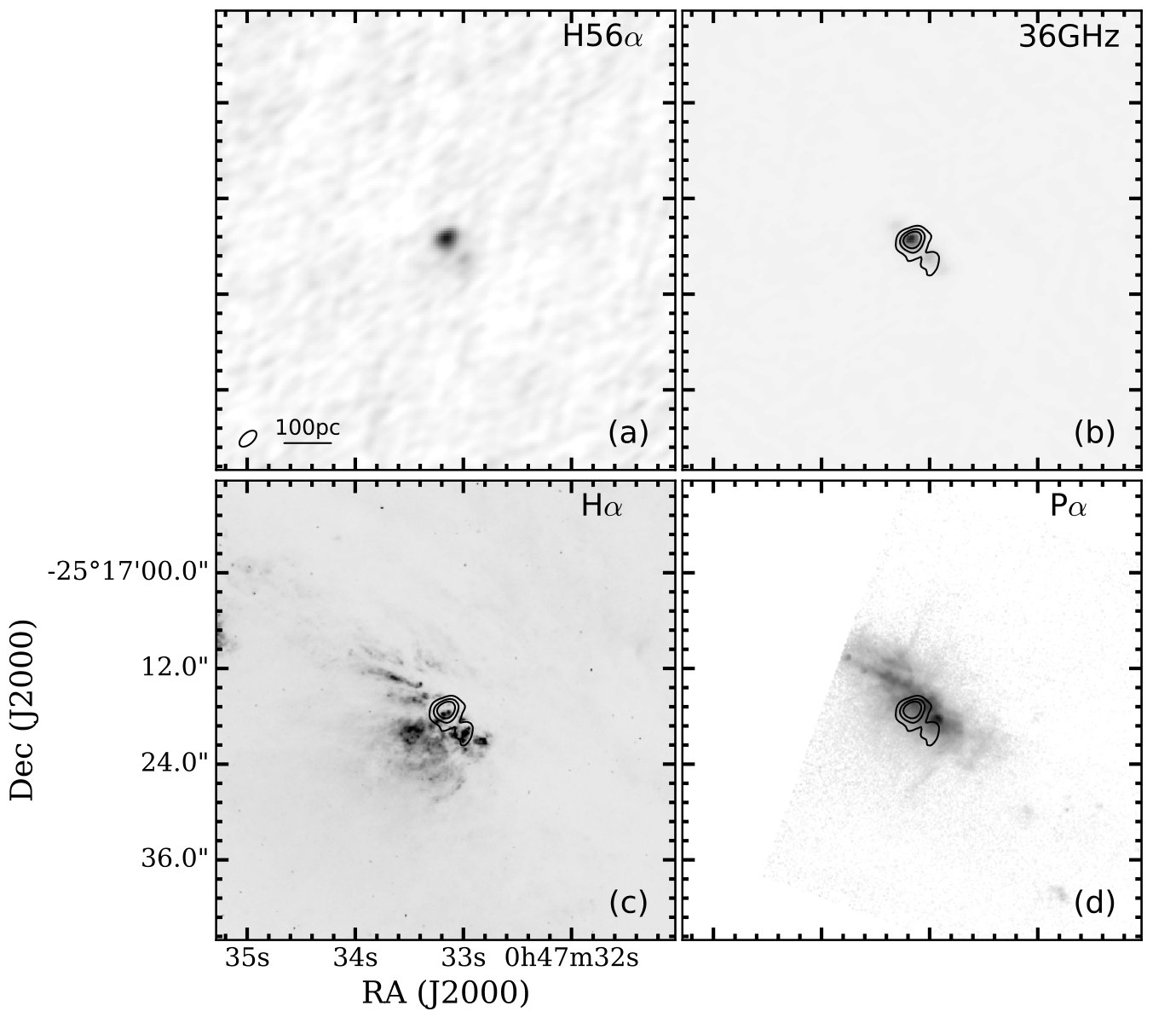 Figure 16
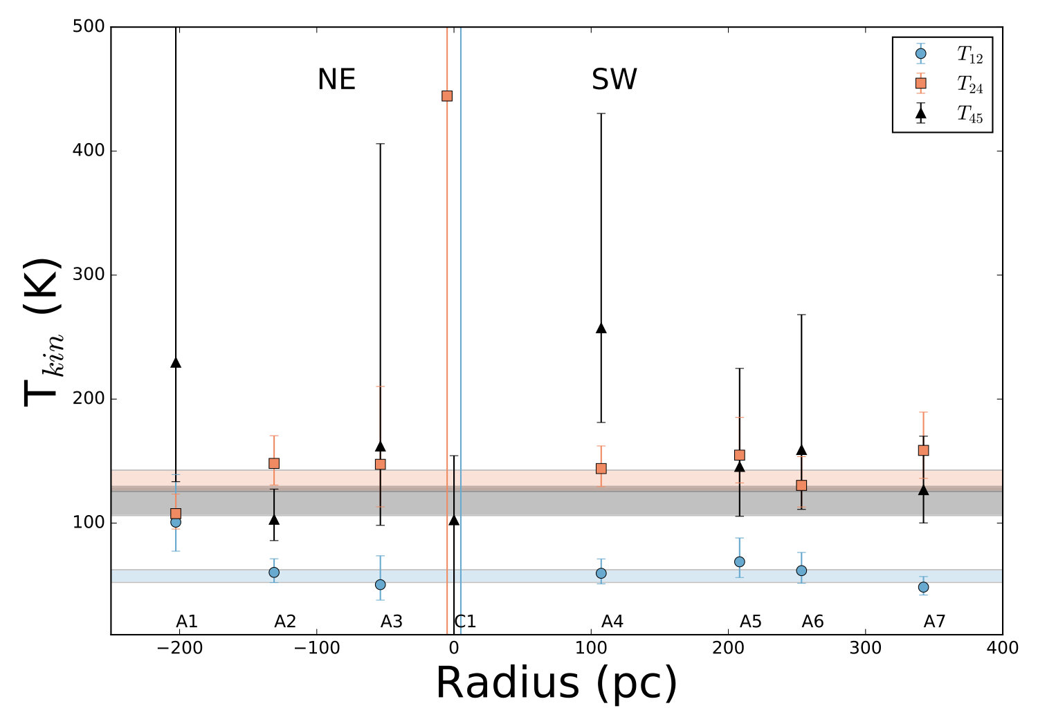 Figure 17
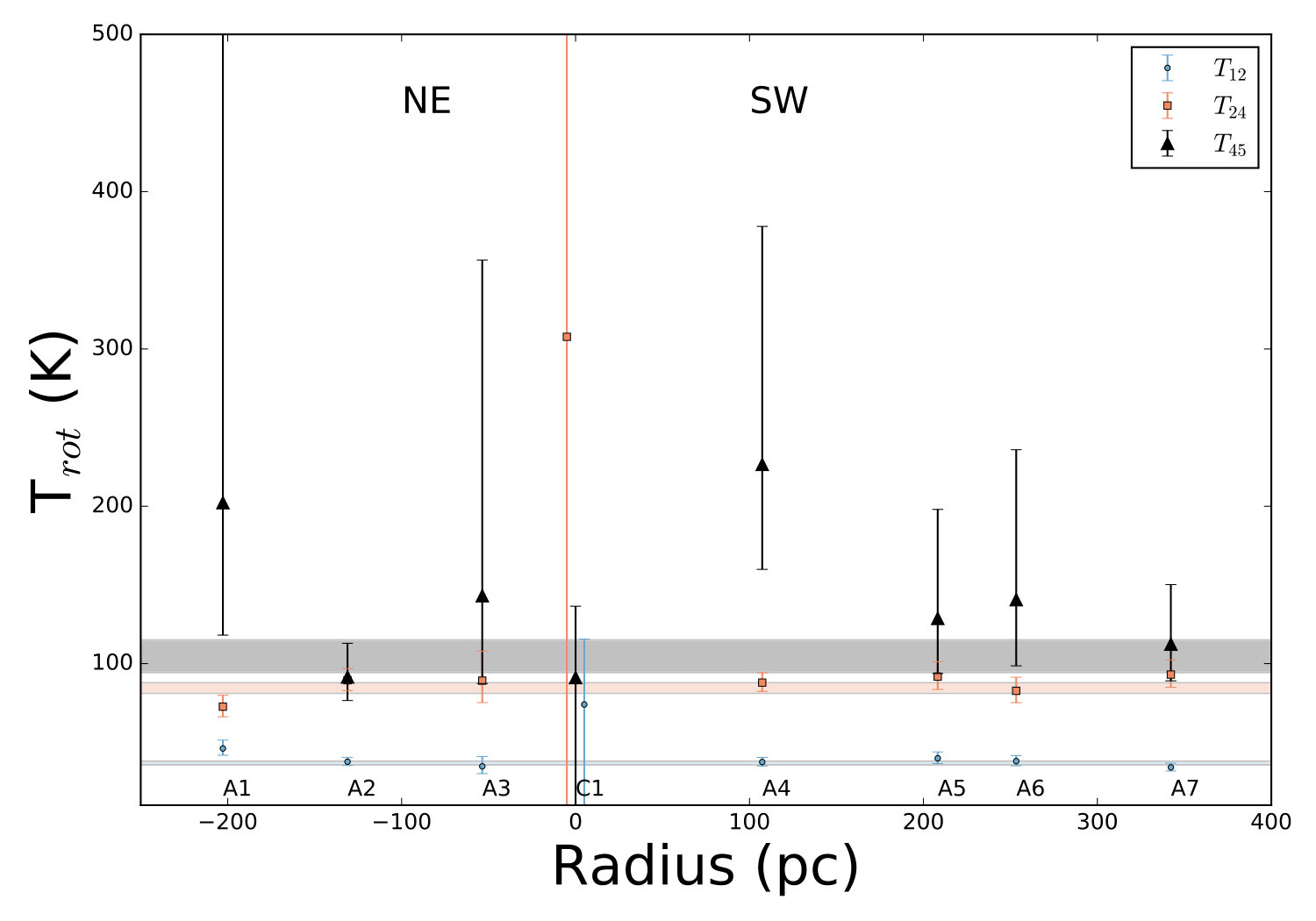 Figure 18
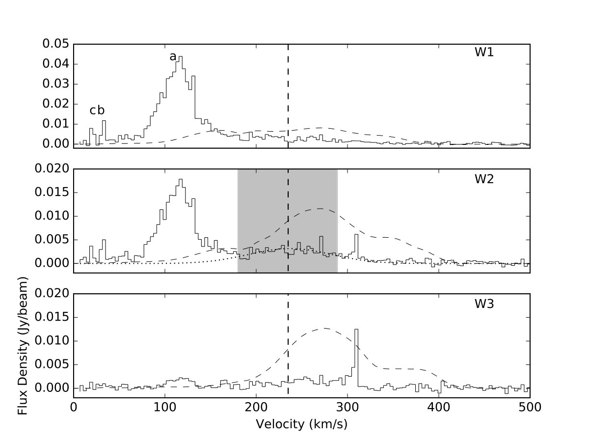 Figure 19
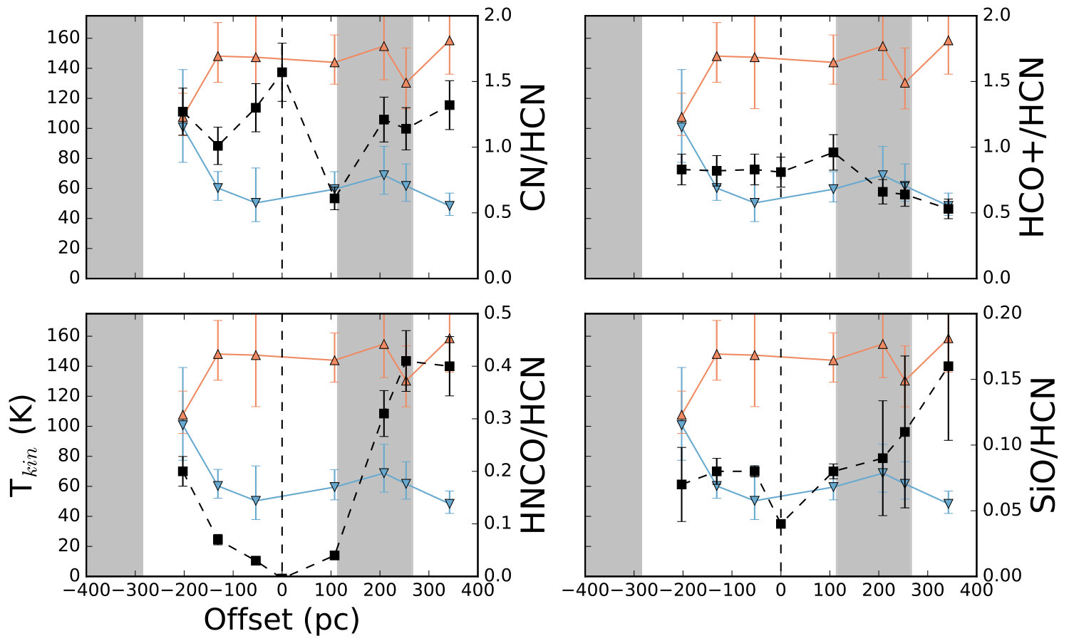 Figure 20
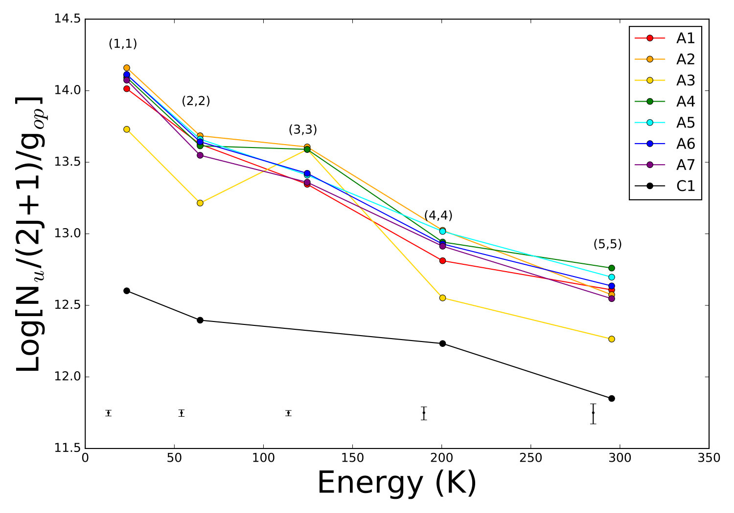 Figure 21
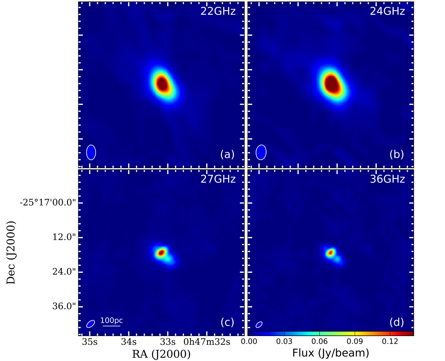 Figure 22
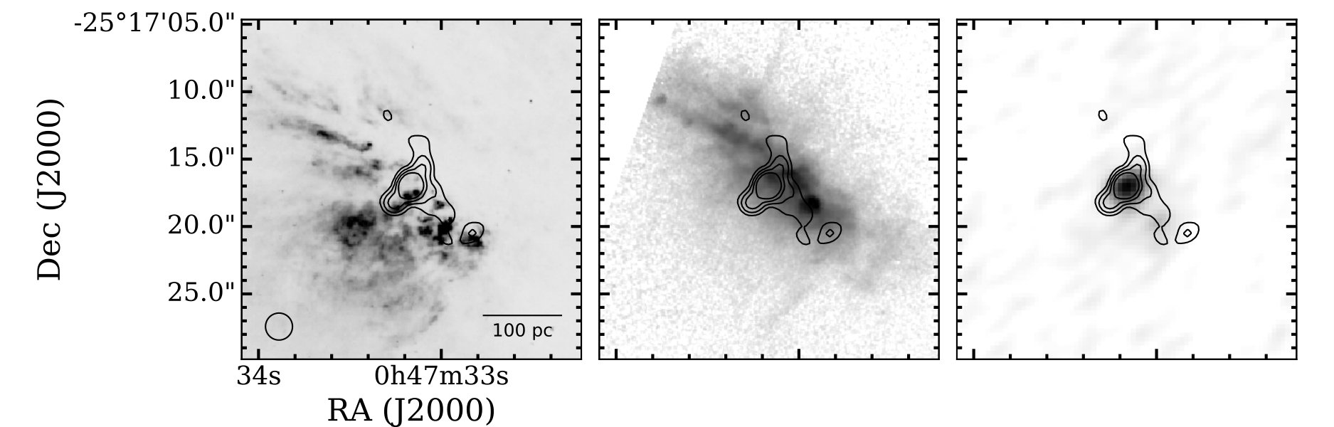 Figure 23
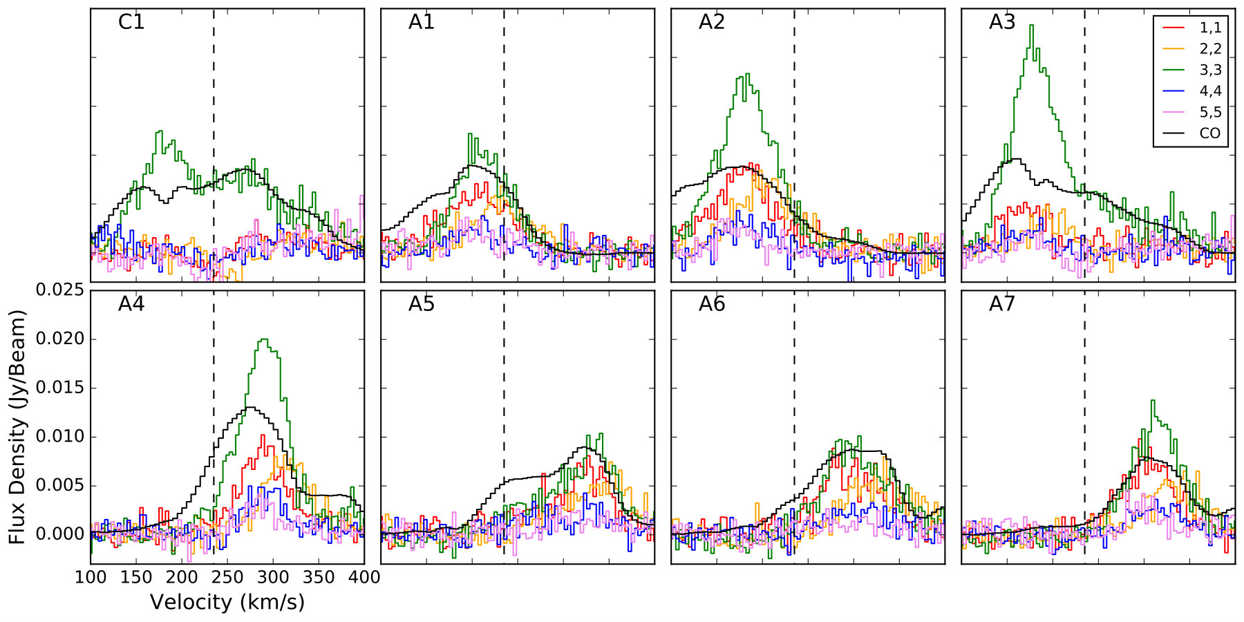 Figure 24
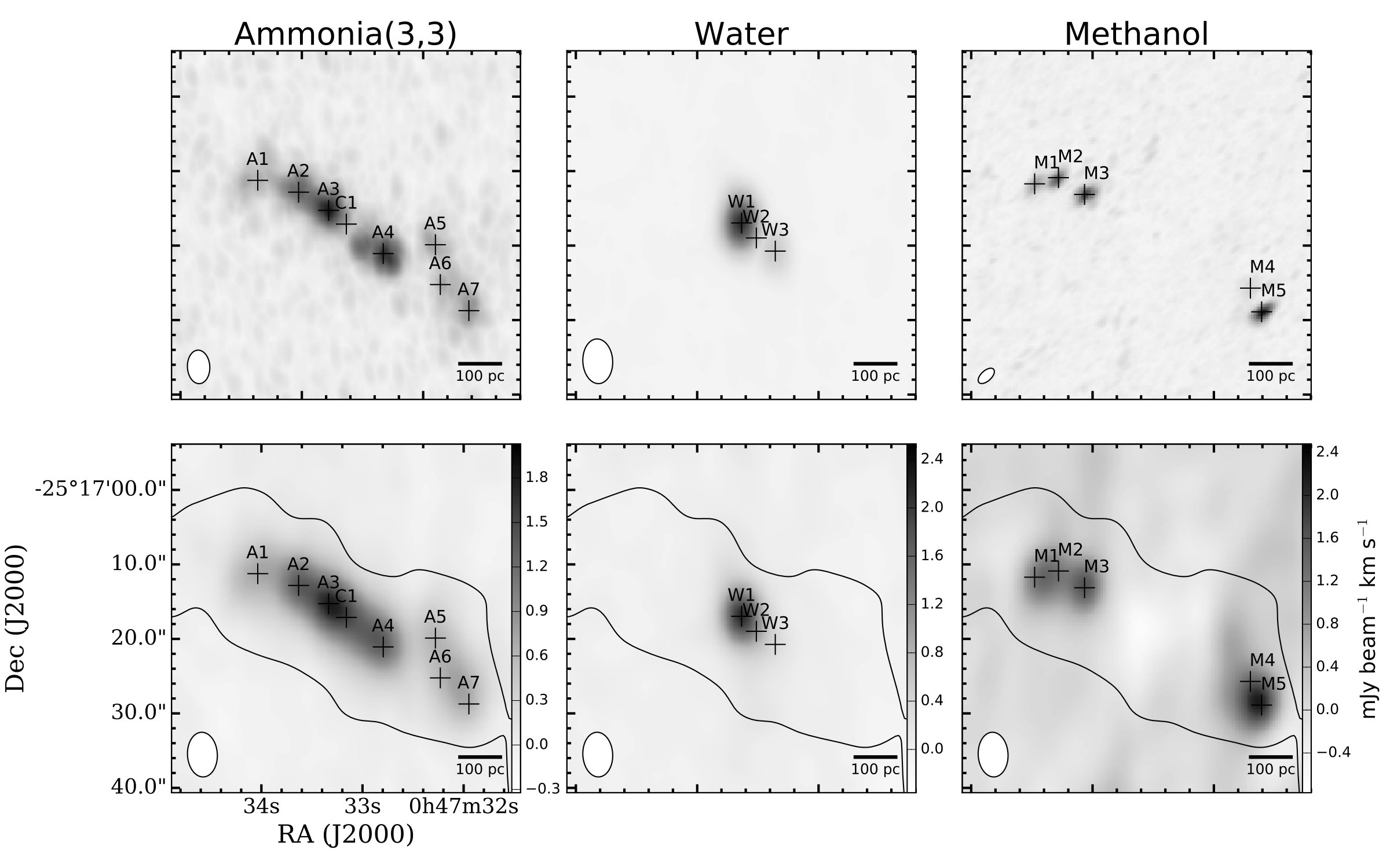 Figure 25
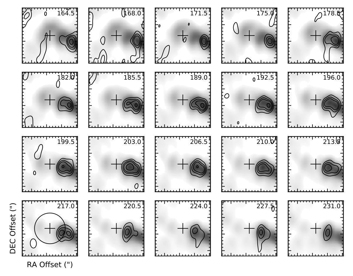 Figure 26
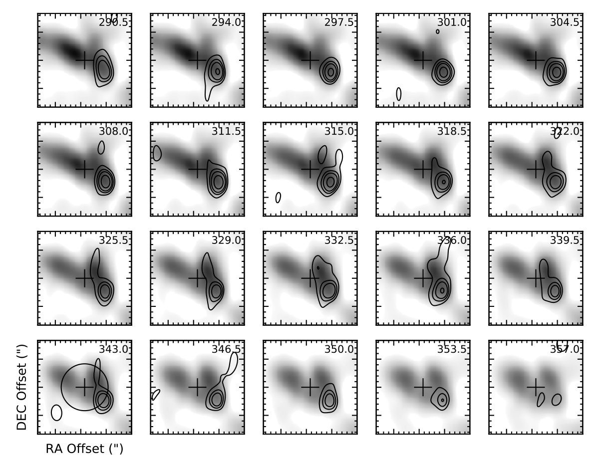 Figure 27
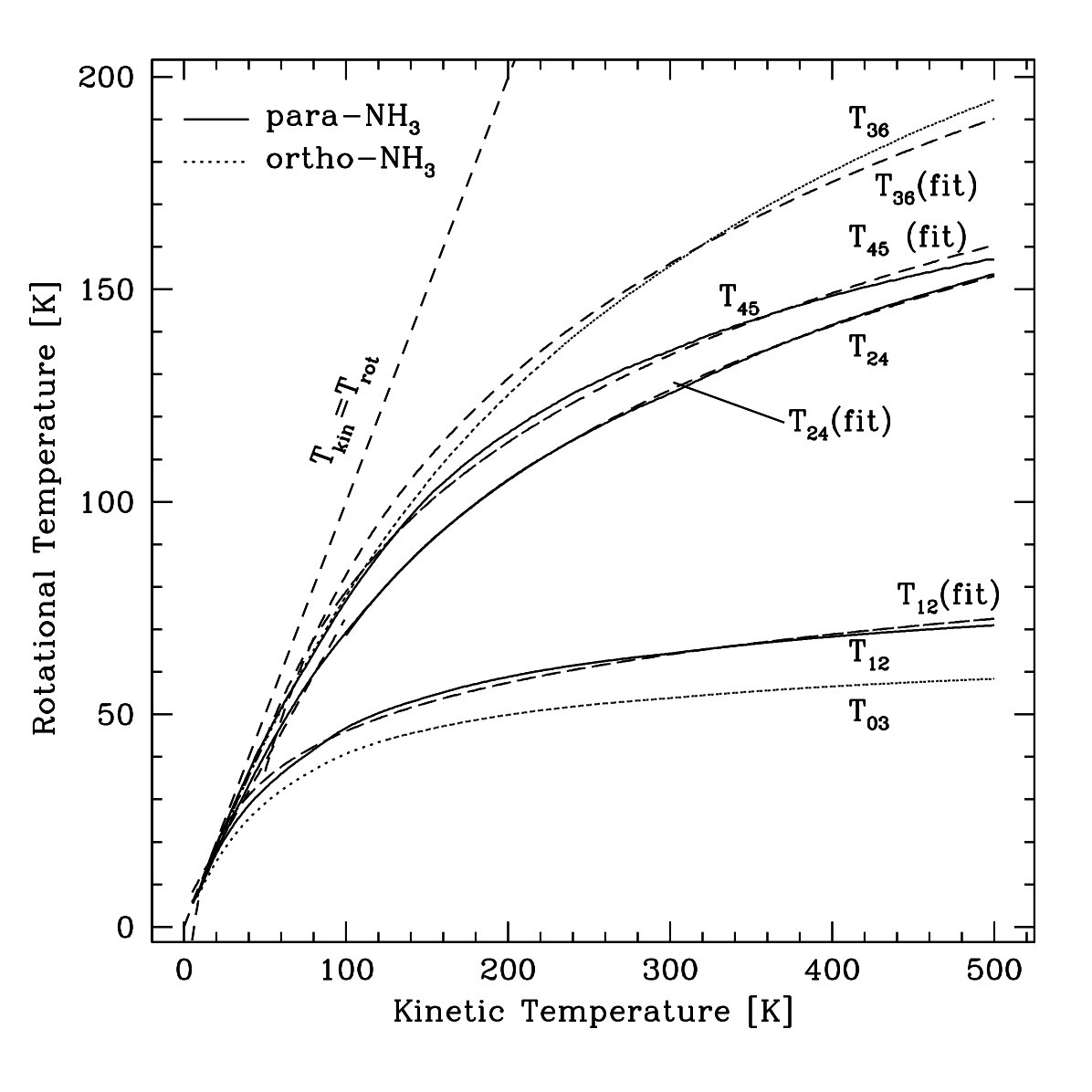 Figure 28
| Transition | Rest Frequency |
|---|---|
| (GHz) | |
| c-C3H2 (220-211) | 21.5874 |
| H2O() | 22.2351 |
| H66 | 22.3642 |
| H64 | 24.5099 |
| NH3 (1,1) | 23.6945 |
| NH3 (2,2) | 23.7226 |
| NH3 (3,3) | 23.8701 |
| NH3 (4,4) | 24.1394 |
| NH3 (5,5) | 24.5330 |
| H62 | 26.9392 |
| c-C3H2 (330-321) | 27.0843 |
| HC3N (3-2) | 27.2944 |
| NH3 (9,9) | 27.4779 |
| CH3OH () | 36.1693 |
| HC3N (4-3) | 36.3924 |
| H56 | 36.4663 |
| CH3CN (2-1) | 36.7956 |
| Location | A1 | A2 | A3 | A4 | A5 | A6 | A7 |
|---|---|---|---|---|---|---|---|
| RA (J2000) hh:mm:ss | 00:47:34.0 | 00:47:33.6 | 00:47:33.3 | 00:47:32.8 | 00:47:32.3 | 00:47:32.2 | 00:47:31.9 |
| DEC (J2000) 0° 0′ 0″ | -25 17 11.2 | -25 17 12.8 | -25 17 15.3 | -25 17 21.1 | -25 17 19.9 | -25 17 25.2 | -25 17 28.7 |
| Distance from C1* (pc) | 202 | 131 | 53 | 107 | 208 | 253 | 342 |
| NH3(1,1) | |||||||
| (K km s-1) | 48.82.1 | 66.82.4 | 24.62.0 | 57.22.2 | 61.03.0 | 62.42.6 | 59.32.3 |
| ( km s-1) | 200.11.8 | 172.81.4 | 62.82.1 | 278.20.1 | 313.22.3 | 294.51.9 | 299.61.4 |
| ( km s-1) | 83.64.2 | 80.83.5 | 54.25.0 | 65.33.2 | 95.26.0 | 90.04.3 | 74.93.5 |
| (K) | 0.550.08 | 0.780.09 | 0.430.09 | 0.810.09 | 0.600.10 | 0.650.09 | 0.740.09 |
| NH3(2,2) | |||||||
| (K km s-1) | 44.42.1 | 49.81.9 | 16.71.7 | 42.41.7 | 48.32.1 | 47.02.3 | 39.32.0 |
| ( km s-1) | 225.42.0 | 198.61.4 | 192.22.6 | 309.51.1 | 336.42.0 | 323.22.3 | 328.51.8 |
| ( km s-1) | 87.15.3 | 73.63.3 | 49.75.6 | 55.12.6 | 89.14.6 | 91.45.1 | 74.34.4 |
| (K) | 0.450.08 | 0.640.08 | 0.320.09 | 0.720.08 | 0.510.08 | 0.480.08 | 0.500.08 |
| NH3(3,3) | |||||||
| (K km s-1) | 74.012.1 | 132.02.3 | 125.53.2 | 126.92.3 | 83.12.4 | 89.92.5 | 80.91.6 |
| ( km s-1) | 204.90.8 | 176.60.6 | 176.20.8 | 283.90.5 | 316.61.4 | 287.91.3 | 308.50.6 |
| ( km s-1) | 68.82.0 | 74.41.4 | 63.72.0 | 61.51.4 | 103.53.7 | 93.73.1 | 66.11.6 |
| (K) | 1.010.07 | 1.390.08 | 1.850.14 | 1.940.10 | 0.780.08 | 0.900.09 | 1.150.07 |
| NH3(4,4) | |||||||
| (K km s-1) | 15.02.1 | 23.91.9 | 008.01.4 | 19.81.3 | 24.12.3 | 20.02.2 | 20.11.7 |
| ( km s-1) | 199.03.7 | 176.92.8 | 166.53.6 | 286.71.6 | 301.95.1 | 300.34.5 | 310.02.8 |
| ( km s-1) | 59.58.6 | 70.56.4 | 36.56.6 | 44.53.3 | 125.413.7 | 82.410.4 | 64.86.2 |
| (K) | 0.240.09 | 0.320.08 | 0.210.08 | 0.410.07 | 0.170.07 | 0.230.08 | 0.290.09 |
| NH3(5,5) | |||||||
| (K km s-1) | 12.12.4 | 11.01.3 | 005.21.3 | 16.91.8 | 15.02.5 | 13.22.2 | 11.21.5 |
| ( km s-1) | 195.96.1 | 164.52.5 | 168.33.7 | 281.42.7 | 316.17.3 | 285.68.3 | 294.22.4 |
| ( km s-1) | 71.519.2 | 40.95.2 | 29.07.7 | 53.97.6 | 91.219.2 | 103.519.6 | 36.55.1 |
| (K) | 0.150.08 | 0.250.08 | 0.170.09 | 0.290.08 | 0.150.09 | 0.120.07 | 0.280.09 |
| Rotation Temperatures | |||||||
| (K) | |||||||
| (K) | |||||||
| (K) | |||||||
| Kinetic Temperatures | |||||||
| (K) | |||||||
| (K) | |||||||
| (K) | |||||||
| NH3 | ||||
|---|---|---|---|---|
| (J,K) | (K km s-1) | ( km s-1) | ( km s-1) | (K) |
| Absorption | ||||
| NH3(1,1) | -8.11.5 | 223.33.4 | 32.36.9 | -0.230.10 |
| NH3(2,2) | -17.51.7 | 247.72.6 | 49.76.6 | -0.330.08 |
| NH3(4,4) | -10.72.4 | 223.86.9 | 60.016.3 | -0.170.11 |
| NH3(5,5) | -6.81.3 | 218.72.9 | 29.46.1 | -0.220.09 |
| Emission | ||||
| NH3(3,3)a | 48.65.1 | 171.11.1 | 55.13.2 | 0.820.09 |
| NH3(3,3)b | 86.76.2 | 256.64.5 | 129.69.5 | 0.630.09 |
| (K km s-1) | 006.91.2 |
| ( km s-1) | 164.73.5 |
| ( km s-1) | 38.16.7 |
| (K) | 0.170.07 |
| RA (J2000) | Dec(J2000) | Velocity Component | Luminosity | ||||
|---|---|---|---|---|---|---|---|
| hh:mm:ss | ° 0′ 0″ | (K km s-1) | ( km s-1) | ( km s-1) | (K) | ||
| W1 | |||||||
| 00:47:33.1 | -25 17 16.9 | a | 214.93.5 | 109.10.3 | 42.00.9 | 4.70.2 | 0.667 |
| b | 006.21.1 | 27.00.4 | 3.50.5 | 1.70.2 | 0.019 | ||
| c | 005.50.1 | 21.0 | 3.5∗ | 1.60.2 | 0.017 | ||
| W2 | |||||||
| 00:47:33.0 | -25 17 19.0 | 25.72.7 | 233.6 | 107.214.0 | 0.20.09 | 0.080 | |
| W3 | |||||||
| 00:47:32.8 | -25 17 20.7 | 7.40.5 | 303.61.4 | 3.51.1 | 2.010.10 | 0.023 | |
| RA(J2000) | Dec(J2000) | Velocity Component | Luminosity | ||||
|---|---|---|---|---|---|---|---|
| hh:mm:ss | ° 0′ 0″ | (K km s-1) | ( km s-1) | ( km s-1) | (K) | ||
| M1 | |||||||
| 00:47:34.1 | -25 17 11.7 | 1.380.07 | 202.00.3 | 49.23.1 | 0.0260.005 | 0.63 | |
| M2 | |||||||
| 00:47:33.9 | -25 17 10.8 | 1.410.07 | 195.40.8 | 32.22.3 | 0.0400.006 | 0.65 | |
| M3 | |||||||
| 00:47:33.7 | -25 17 13.1 | 3.590.14 | 165.91.7 | 85.84.4 | 0.0390.008 | 1.63 | |
| M4 | |||||||
| 00:47:31.9 | -25 17 28.9 | 3.090.18 | 294.12.6 | 84.35.6 | 0.0350.005 | 1.42 | |
| M5 | |||||||
| 00:47:32.0 | -25 17 25.7 | a | 2.190.89 | 294.33.0 | 35.74.8 | 0.0560.005 | 1.01 |
| b | 2.330.96 | 331.610.2 | 54.516.9 | 0.0410.005 | 1.06 | ||
| Location | A1 | A2 | A3 | A4 | A5 | A6 | A7 |
|---|---|---|---|---|---|---|---|
| NH3(1,1)/NH3(2,2) | |||||||
| (K) | 117 135 | 6924 | 5427 | 6924 | 8141 | 72 27 | 57 18 |
| NH3(2,2)/NH3(4,4) | |||||||
| (K) | 11124 | 15639 | 16575 | 15033 | 16548 | 10824 | 16242 |
Peer Reviews
No public reviews on file for this paper yet. If you reviewed it on a platform where reviews are public (OpenReview, ICLR, NeurIPS, ICML), you can paste yours below so the community can read it here.
Videos
No videos yet. Explain this paper in a talk, walkthrough, or lecture? Add one.
Survey of Water and Ammonia in Nearby galaxies (SWAN): Resolved Ammonia Thermometry, Water and Methanol Masers in the Nuclear Starburst of NGC 253
Mark Gorski11affiliationmark: 22affiliationmark:
Jürgen Ott11affiliationmark:
Richard Rand22affiliationmark:
David S. Meier33affiliationmark: 11affiliationmark:
Emmanuel Momjian11affiliationmark:
Eva Schinnerer44affiliationmark:
1 National Radio Astronomy Observatory, P.O. Box O, 1003 Lopezville Road, Socorro, NM 87801, USA
2 Department of Physics and Astronomy, University of New Mexico, 1919 Lomas Blvd NE, Albuquerque, NM 87131, USA
3 Department of Physics, New Mexico Institute of Mining and Technology, 801 Leroy Place, Socorro, NM 87801, USA
4 Max-Planck Institut für Astronomie, Königstuhl 17, D-69117 Heidelberg, Germany
Abstract
We present Karl G Jansky Very Large Array molecular line observations of the nearby starburst galaxy NGC 253, from SWAN: ”Survey of Water and Ammonia in Nearby galaxies”. SWAN is a molecular line survey at centimeter wavelengths designed to reveal the physical conditions of star forming gas over a range of star forming galaxies. NGC 253 has been observed in four 1GHz bands from 21 to 36 GHz at 6″ pc) spatial and 3.5 km s*-1spectral resolution. In total we detect 19 transitions from seven molecular and atomic species. We have targeted the metastable inversion transitions of ammonia (NH3*) from (1,1) to (5,5) and the (9,9) line, the 22.2 GHz water (H2O) () maser, and the 36.1 GHz methanol (CH3OH) () maser. Utilizing NH3 as a thermometer, we present evidence for uniform heating over the central kpc of NGC 253. The molecular gas is best described by a two kinetic temperature model with a warm 130K and a cooler 57K component. A comparison of these observations with previous ALMA results suggests that the molecular gas is not heated in photon dominated regions or shocks. It is possible that the gas is heated by turbulence or cosmic rays. In the galaxy center we find evidence for NH3(3,3) masers. Furthermore we present velocities and luminosities of three water maser features related to the nuclear starburst. We partially resolve CH3OH masers seen at the edges of the bright molecular emission, which coincides with expanding molecular superbubbles. This suggests that the masers are pumped by weak shocks in the bubble surfaces.
\submitted
Accepted for publication in the Astrophysical Journal
1 Introduction
Physical descriptions of how the Interstellar Medium (ISM) condenses to form stars, and the resulting feedback from star formation, limit our understanding of galaxy evolution and the star formation history of the universe. Models of galaxy evolution without feedback drastically over predict star formation rates and efficiencies. Feedback is necessary to impede star formation otherwise a galaxy reach its peak star formation rate in less than a dynamical time and quickly convert its baryons to stars shortly after (e.g. Kauffmann et al. 1999; Krumholz et al. 2011; Hopkins et al. 2011). Star formation is largely correlated with the amount of dense, cm*-3*, molecular gas within a galaxy (e.g. Gao & Solomon 2004), and in simulations the state of such gas is limited by the resolution of each individual simulation, i.e. subgrid physics (e.g. Okamoto et al. 2005; Haas et al. 2013; Crain et al. 2015). Consequently, understanding the relationship between star formation, the resulting feedback, and the state of the dense molecular gas is critical to understanding the star formation history of a galaxy.
Feedback in the star forming ISM perturbs molecular gas such that it can no longer collapse and form new stars. Heating from supernovae, stellar winds, and photoionization are examples of the most dominant forms of stellar feedback (e.g. Kauffmann et al. 1999, Hartmann et al. 2001, & Vázquez-Semadeni et al. 2010). One dimensional simulations by Murray et al. (2010) suggest that different mechanisms dominate at different times during the lifetime of star forming Giant Molecular Clouds (GMCs). Furthermore, simulations by Hopkins et al. (2012) and Hopkins et al. (2014) show that these different feedback effects compound in a non-linear way and that no single feedback process dominates the star forming ISM. Additionally, the environment in which star forming material exists may play a critical role in its properties. Therefore, observational constraints are necessary to refine the subgrid physics within the theoretical models on the appropriate scales.
Nearby galaxies provide access to scales of tens of pc where observations can reveal how feedback operates. There are many studies that look at different aspects of feedback. For example in NGC 253 Strickland et al. (2002) and Westmoquette et al. (2011) discuss the X-ray and ionized gas properties of a starburst driven outflow, respectively. Studies of NH3, such as those by Ott et al. (2005), Lebrón et al. (2011) and Mangum et al. (2013), reveal heating and cooling of the molecular ISM. In addition, other molecular tracers reveal shocks, Photon Dominated Regions (PDRs), masses, lengths and time scales associated with star formation. (e.g. Meier et al. 2015, Leroy et al. 2015).
The “Survey of Water and Ammonia in Nearby galaxies” (SWAN) is a survey of molecular line tracers at centimeter wavelengths designed to reveal the physical conditions in star forming gas. The sample consists of four star forming galaxies: NGC 253, IC 342, NGC 6946, and NGC 2146, and was chosen to span a range of galaxy types from Milky Way-like to starbursts and an order of magnitude of star formation rates from ( M*⊙* yr*-1*) to starbursts (10 M*⊙* yr*-1*). Here we discuss the first results from SWAN focusing on VLA K- and Ka-band observations of NGC 253.
NGC 253 has been studied at many wavelengths: X-ray (e.g. Strickland et al. 2002), optical (e.g. Westmoquette et al. 2011), infrared (e.g. Dale et al. 2009), millimeter (e.g. Bolatto et al. 2013 & Meier et al. 2015), and radio (e.g. Ulvestad & Antonucci 1997). Figure 1 shows a Spitzer 8m image of NGC 253 (Dale et al., 2009). The inset shows the central kpc with 3, 6 and 9 contours of NH3(3,3) emission from our data discussed in Section 3.2.1. We adopt a distance of 3.5 Mpc measured from the tip of the red giant branch (Radburn-Smith et al., 2011) and a systemic velocity of 234 km s*-1* in the LSRK frame from Whiting (1999). All velocities in this paper will be in the LSRK frame unless otherwise stated. The disk is inclined at i78*∘* (Pence, 1980). NGC 253 has a total star formation rate (SFR) of 5.9 M*⊙* yr*-1* of which approximately half is concentrated into the central kpc (McCormick et al., 2013). The starburst is driving a massive molecular outflow, with a mass-loss rate estimated at 9 M*⊙* yr*-1*, that is thought to be starving the current star forming event (Bolatto et al., 2013). The outflow is also seen in X-rays (Strickland et al., 2002) and H (Watson et al., 1996). Sakamoto et al. (2006) found evidence for two expanding molecular superbubbles within the central kpc with kinetic energies of order J. Ott et al. (2005) and Bolatto et al. (2013) found several smaller molecular superbubbles in the same region. Bolatto et al. (2013) suggest that superbubbles and supernovae from the starburst drive the wind, whereas Westmoquette et al. (2011) favor a cosmic ray driven wind on the larger scales with a small contribution from the starburst in the center, with the molecular gas in the center responsible for collimating the outflow.
Centimeter and millimeter wavelength spectra of galaxies provide access to diagnostically important molecular tracers. The molecular gas is often well traced by CO, however more complex molecules can provide better tracers of gas properties such as temperature and density, and can be used to trace specific conditions such as PDRs and shocks (e.g. Fuente et al. 1993, García-Burillo et al. 2000, Meier & Turner 2005, and Meier et al. 2015). This study will focus on the metastable transitions (J=K) (1,1) to (5,5) and (9,9) of NH3, the 22 GHz H2O() maser, and the 36 GHz CH3OH() maser. We will use a combined analysis of these lines to expose the processes that dominate the central kpc of NGC 253.
The NH3 molecule generally works well as a temperature tracer of the molecular gas. The tetrahedral structure of NH3 makes it a symmetric top, meaning the energy states are described by the rotation angular momentum quantum number J and the projection along the symmetry axis K. The J=K states, called metastable states, are long lived compared to JK states, and population exchanges between K ladders are forbidden except by collisions. Therefore when NH3 is collisionally excited ( critical density n cm*-3*) the K ladders are expected to be populated in accordance with the kinetic temperature of the gas. As a result, measurements of the relative intensities of metastable states act as probes of the rotation temperature of the gas (e.g. Ho & Townes 1983, Walmsley & Ungerechts 1983, Lebrón et al. 2011, Ott et al. 2005, Ott et al. 2011, and Mangum et al. 2013).
The NH3(3,3) state can be a maser transition (Walmsley & Ungerechts, 1983), but it is less well studied than other masers. In the Galaxy there is a weak association of NH3(3,3) masers with dense gas in star forming regions (e.g. Wilson & Mauersberger 1990, Mills & Morris 2013, and Goddi et al. 2015). Here we will use metastable transitions of NH3 to understand the heating and cooling balance of the dense molecular ISM in NGC 253.
The H2O and CH3OH masers provide a unique opportunity to probe star forming environments. The H2O line requires gas densities cm*-3* and kinetic temperatures K to mase (e.g. Tarchi 2012). In the Galaxy these masers are typically found in shocked regions around Young Stellar Objects (YSOs) and Asymptotic Giant Branch (AGB) stars (e.g. Palagi et al. 1993) and may be used to identify regions of hot, dense, and/or shocked gas. This is in addition to precisely tracing kinematics of stellar winds (e.g. Goddi & Moscadelli 2006), and accretion disks (e.g. Peck et al. 2003; Lo 2005; Reid et al. 2009).
Class I (collisionally pumped) and II (radiatively pumped) CH3OH masers are found in high mass star forming regions (e.g. Ellingsen et al. 2012) and supernova remnants (e.g. McEwen et al. 2014)in the Galaxy. The Class I masers trace shocks and gas densities cm*-3* (Pratap et al., 2008). The 36.2 GHz CH3OH line studied here is a Class I type maser. We will mostly use these masers as signposts of shocked material.
In §2 we describe the observational setup. In §3 we report our measurements of the NH3, H2O, and CH3OH lines in addition to a brief description of the continuum and the H56 Radio Recombination Line (RRL). In §4 we discuss the derivation of temperatures across the molecular bar, the relevance of the H2O masers to the outflow, the significance of the CH3OH masers, and a comparison with previous ALMA millimeter molecular lines. Lastly, we summarize our findings in §5.
2 Observations and Data Reduction
We observed NGC 253 with the 18-26.5 GHz and 26.5-40 GHz (K- and Ka-bands) receivers of the Karl G. Jansky Very Large Array (VLA)111The National Radio Astronomy Observatory is a facility of the National Science Foundation operated under cooperative agreement by Associated Universities, Inc. (project code: 13A-375). The K-band observations were carried out on 2013 May 11. The Ka-band observations were split into two sessions: 2013 May 23 and 2013 May 26. The VLA was in the DnC hybrid configuration for all these observations. This configuration delivers a rounder beam for low declination sources because the north arm is in the more extended C configuration, while the east and west arms are in D configuration. The received signal is sampled at each antenna using the 8-bit samplers. These provide two 1 GHz baseband pairs with both right and left hand circular polarizations. The correlator was set up to divide each baseband into 8 sub-bands each with 512 channels resulting in a channel width of 250kHz. This yields a velocity resolution ranging from 3.0 to 3.3 km s*-1* for the K-band, and 2.0 to 2.7 km s*-1* for the Ka-band observations. The baseband pairs were centered at 21.8 GHz and 24.1 GHz in K-band, 27.1 GHz and 36.4 GHz in Ka-band. They will be referred to as the 22 GHz, 24 GHz, 27 GHz, and 36 GHz basebands, respectively. These were chosen to include the metastable NH3 transitions from (1,1) with rest frequency 26.6946 GHz, to (5,5) at 24.5330 GHz, as well as (9,9) at 27.4779 GHz, the H2O() maser line at 22.2351 GHz, and the CH3OH() transition at 36.1693 GHz. All of the detected lines and their rest frequencies are listed in Table 1. The on source time for the K-band and Ka-band observations was 4.4 hours and 3.6 hours, respectively. We used 3C48 as the flux density calibrator Perley & Butler (2013), J2253+1608 as the bandpass calibrator, and J0025-2602 as the complex gain calibrator in all observations. We alternated between 10 minute intervals on NGC 253 and 1.5 minute intervals on the complex gain calibrator.
The data were reduced in the Common Astronomy Software Applications (CASA) package version 4.2.2 (McMullin et al., 2007). At the adopted distance of 3.5 Mpc the linear scale is 17 pc per arcsecond. The half power primary beam widths of the VLA for the K- and Ka-bands are 2.1′ (2 kpc) and 1.5′ (1.5 kpc) respectively. All data cubes were gridded with 0.25″ pixels, mapped using natural weighting, CLEANed to rms noise, and are regridded to a common velocity resolution of 3.5 km s*-1*. Continuum subtraction was performed in the UV domain. For the 24 GHz baseband, several baselines were flagged for being noisy yielding a slightly larger synthesized beam than the 22GHz baseband. The resulting image cubes are then smoothed to a common synthesized beam of 6″4″ (Position Angle: 3.00*∘). The common resolution cubes are used for consistency for all the observed lines. The resulting rms noise values in the K-band and Ka-band image cubes are 0.5 mJy beam-1* and 1 mJy beam*-1* in a 3.5 km s*-1* channel, respectively. The maser lines of H2O, CH3OH, and NH3(3,3) have also been imaged with 0.25″ pixels and Briggs (robust=0) weighting, yielding a synthesized beam of 4″3″ for H2O and NH3(3,3) and 2″1″ for CH3OH, to better constrain the locations of masing material. The rms noise in the K-band and Ka-band Briggs weighted image cubes are 1.5 mJy beam*-1* and 3.1 mJy beam*-1* in a 3.5 km s*-1* channel, respectively. A super-resolved cube was constructed for the H2O maser data. This was done by deconvolving a dirty image cube then convolving the CLEAN components with a 1″ round beam. This super-resolved image cube is used to emphasize structures seen in the CLEAN components that are difficult to discern in the regularly resolved image cubes. No quantitative measurements are made with the super-resolved cube.
3 Results
The full continuum subtracted spectra of our K- and Ka-band observations are presented in Figure 2. We have identified 17 transitions from seven different molecular or atomic species shown in Table 1. Lines were identified by searching the common resolution data cubes with a pixel sized beam. We set conservative conditions for a detection at a peak flux of 1.5 mJy beam*-1* channel*-1* for K-band and 3.0 mJy beam*-1* channel*-1* for Ka-band, and a FWHM of 30 km s*-1* for thermal lines. For known maser transitions single channels above 6 are considered detections.
3.1 Continuum Emission and Radio Recombination Lines
The radio continuum emission from NGC 253 is resolved in all four basebands (Figure 3). Images were made selecting only line free channels. The flux density measured in the 24 GHz baseband is 55030 mJy. This agrees with the value of 52052 mJy from Ott et al. (2005). The 36 GHz flux density measures 35040 mJy in close agreement with the value of 330 mJy at 32 GHz measured by Kepley et al. (2011). The other continuum flux density measurements are 47020 mJy and 37040 mJy for the 22 GHz and 27 GHz basebands, respectively. The spectral index derived from the K-band basebands is 0.5 and for Ka-band . The measurements suggest the continuum goes through a minimum between the 24 GHz and 27 GHz basebands. The H56 transition is the strongest radio recombination line (RRL) we detect. Figure 4 shows the relationship between the Hubble (HST) H (Watson et al., 1996), H56, Pa (Alonso-Herrero et al., 2003), and the 36 GHz continuum emission. We treat the H as a tracer of the outflow with heavy dust obscuration, Pa as a partially obscured star formation tracer and RRL as an unobscured star formation tracer.
3.2 Molecular Emission Lines
Our analysis from here on will focus only on NH3, H2O, and CH3OH. These transitions are shown in bold text in Table 1. Intensity and peak flux maps are shown in Figure 5. Spectra have been extracted from the naturally weighted, smoothed cubes from the pixels at the locations marked by crosses (Figure 5) and are shown in Figures 6, 7, and 8. These locations were selected from the spatial peaks in the peak flux maps shown, or for spectrally unique characteristics. For example, W2 is not a spatial peak in the peak flux map but was selected for a spectral component discussed in Section 3.2.2. The continuum peak is labeled C1, and identifies the starburst center. The NH3 locations are labeled A1-A7. We use the NH3(3,3) line to select a representative sample of locations across NGC 253 because it is the strongest observed NH3 transition. Locations for H2O and CH3OH are labeled with W and M, respectively.
3.2.1 NH3 Inversion Lines
The observed NH3 emission spans an elongated structure 1 kpc in length about the continuum peak. The northeast (NE) side of the continuum peak contains three NH3(3,3) spatial peaks (A1, A2 & A3), which are blueshifted from the systemic velocity with observed velocities ranging from km s*-1* to 200 km s*-1*.The southwest (SW) side of the continuum peak contains four NH3(3,3) peaks (A4, A5, A6, & A7), which are redshifted from systemic with velocities ranging from km s*-1* to 320 km s*-1*. (Figure 5). The peaks A1, A2, & A3 can be cross-identified with in regions F, E, and D from Ott et al. (2005) and A4, A5, A6 and A7 are analogous to C, B, and A . It should be noted that this is not a one to one mapping as we have a smaller beam than the superresolved cube used in Ott et al. (2005). The NH3 spectra from each pixel are shown in Figure 6. We detect inversion transitions NH3(1,1) to (5,5) at all locations. In addition the NH3(9,9) line is weakly detected at site A3 (spectrum not shown). At the continuum peak all the NH3 transitions are seen in absorption with the exception of NH3(3,3). Single Gaussians were fitted to the spectrum extracted from each location, from which we extract the integrated flux, peak flux, FWHM, and the line center, from the individual pixels marked in Figure 5. The properties of the metastable transitions, NH3(1,1) to (5,5), for A1-A7 are listed in Table 2 and C1 in Table 3. The weakly detected NH3(9,9) fit results are listed in Table 4. We do not see the NH3 metastable inversion hyperfine transitions (J=K, F = 1) as the lines are likely weak and broad enough to be smeared out.
A1, A5 and A6 FWHMs are a few tens of km s*-1* wider than the other locations. These three sites are located on the edges of superbubbles (See section 4.4) discovered by Sakamoto et al. (2006). At C1, the NH3(3,3) line appears in emission whereas all other inversion lines appear in absorption (Figure 6), interpreted to be due to the existence of NH3(3,3) masers, confirming the result from Ott et al. (2005). The NH3(3,3) emission for C1 is not well described by a single Gaussian and thus two Gaussians were fit to the data (Figure 9), with FWHMs of 553 km s*-1* and 13010 km s*-1* and centers of 1721 km s*-1* and 2575 km s*-1*, respectively NH3(3,3)a and NH3(3,3)b.
3.2.2 H2O masers
We identify three regions of H2O maser emission in the data cube, labeled W1 to W3 in Figure 5 (center). The W1 water maser has been previously observed by Henkel et al. (2004) and Brunthaler et al. (2009). Spectra at these positions are shown in Figure 7. Regions W1 and W3 are seen as clear, spatially resolved peaks in Figure 5. Region W1 shows multiple velocity components with the main peak labeled W1a, and the minor peaks labeled W1b and W1c. W2 is a faint feature which is not spatially resolved from W1 and W3, but marks the peak emission of a unique broad component shown by the shaded region in Figure 7. W2 is identified by the peak emission from the narrow feature at 273 km s*-1* channel (Figure 7). W1 and W2 show multiple peaks in the spectrum. These were fitted with single Gaussians where appropriate. The properties are listed in Table 5. Single channel features are likely real, given our spectral resolution, but, were not fitted by Gaussians and thus their FWHMs are upper limits.
The spectrum of W2 has contributions from W1 and W3 as they are not resolved from W2. W2 is a broad pedestal spanning 100 km s*-1* centered at 233 km s*-1* with several narrow features. The rest of its properties are listed in Table 5. This component is much better matched to systemic velocity of NGC 253. W3 is a redshifted single velocity component maser at 303 km s*-1*.
W1a dominates region W1 and is blueshifted with respect to systemic with an observed velocity of 109 km s*-1*. The integrated flux density of the W1a maser is K km s*-1* yielding a luminosity of 0.66 L*⊙making it a kilomaser. The extension is hard to discern in the the peak flux density and integrated flux maps (Figure 5), but it is clearly seen in the contours of the super-resolved image in Figure 10, where contours of the super-resolved image cube are plotted on the HST H, P, and the RRL H56 images. The super-resolved H2O contours show the extension perpendicular to the major axis of NGC 253. This may indicate the W1 H2O masers are related to the outflow of NGC 253 whereas W2 and W3 are spatially more consistent with the nuclear material. This result needs to be confirmed with higher resolution data. Lastly, we do not detect the 145 mJy km s-1* H2O maser dubbed H2O-2 from Henkel et al. (2004) observed in September 2002. H2O masers associated with YSOs and AGB stars can be variable on time scales of months (e.g. Claussen et al. 1996, Felli et al. 2007), therefore a non-detection is unsurprising.
3.2.3 36 GHz CH3OH masers
Extragalactic 36 GHz CH3OH masers were first detected by Ellingsen et al. (2014) in NGC 253 with the Australia Telescope Compact Array (ATCA)222The Australia Telescope Compact Array is part of the Australia Telescope, which is funded by the Commonwealth of Australia for operation as a National Facility managed by CSIRO. with a 8.0″4.2″ synthesized beam. Two sources were detected. The emission is likely not thermal in its nature, despite the large FWHM of the line, due to the total integrated intensity being 20 times greater than the total integrated intensity from the Galaxy’s central molecular zone (see Ellingsen et al. 2014). We resolve the two regions previously seen in Ellingsen et al. 2014 into five different regions with masersas marked in the peak flux map.The spectra are extracted from the common resolution (6″4″) image cubes and shown in Figure 8. The pairs M1 and M2, and M4 and M5 are not spatially resolved from each other in the common resolution cube. M1 and M2 are spectrally similar, however M4 and M5 show distinct spectral components. The CH3OH line is very close to the edge of one of our spectral sub-bands. There are small (3.5 km s*-1*) gaps between each sub-band where the data collected is untrustworthy, thus the channel corresponding to 160 km s*-1* is lost. The data in this channel and the two adjacent channels are thus unreliable. We next fit single component Gaussians where appropriate. The extracted properties of the lines are shown in Table 6. The region M5 was fit with two Gaussians due to the double peak. The spectral features are narrower than the NH3 (this paper) and features (Bolatto et al., 2013) from the same locations, with measured FWHMs spanning a range of 30-80 km s*-1*. The narrower widths suggest that the 36 GHz CH3OH emission is not tracing the entirety of the molecular gas.
4 Discussion
4.1 NH3 Temperatures
One advantage of observing NH3 is that many of its transitions are close in frequency space, and therefore can be observed with single telescope, a single observational setup, and under the same atmospheric conditions. In addition, the % change in frequency between the transitions means that their respective uv coverage and the flux they resolve out are nearly identical. Rotation temperatures can then be derived from as many pairs of metastable (J = K) states as have been observed. Assuming optically thin conditions upper level column densities may be determined from:
[TABLE]
where is the main beam brightness temperature, the column density of the upper inversion state, , is in cm*-2*, and the frequency () is in GHz. A rotation temperature (T) is derived from a pair of the metastable states (J and J′) by:
[TABLE]
where the difference in energy between states J and J′, , is in K (the corrected version of the equation in Henkel et al. 2000 as shown in Ott et al. 2005) and the are statistical weights depending on the NH3 species ( = 1 for para-NH3 and Jn where n is an integer, and = 2 for ortho-NH3 with J=3n). Rotation temperatures derived from pairs of NH3 transitions, for locations A1 to A7 are shown in Table 2. The rotation temperatures are best illustrated in the Boltzmann diagram shown in Figure 12 (top). We have plotted weighted column densities on the vertical axis and energy above the ground state on the horizontal axis. The slopes between any two points are thus proportional to the inverse rotation temperature, i.e. cold gas shows steeper slopes than warm gas (Equation 2). Notice at location C1 we see NH3 in absorption against the continuum (Figure 6) and thus the rotation temperature must be measured differently (see next paragraph). A3 is located beams (53 pc) from C1, thus the emission line is likely partially absorbed, making rotation temperature measurements here unreliable.
Measuring rotation temperatures from NH3 absorption is not possible without knowing the excitation temperature and the optical depth . Huettemeister et al. (1995) describes the process of extracting total NH3 column densities N(J,K) (the sum of both the upper and lower inversion states):
[TABLE]
and,
[TABLE]
where the units of (FWHM) are km s*-1*, and are brightness temperatures of the line and continuum, respectively, and is the optical depth. We have no means to measure the transition-dependent excitation temperature, so for simplicity we assume that for each metastable transition is equal. In this case the rotation temperature can still be derived from Equation 2 by substituting N(J,K) for Nu(J,K). Rotation temperatures for C1 are shown in Table 3. Since the column density at C1 depends on the excitation temperature, the values plotted for C1 in Figure 12 are really N(J,K)/. The spatial dependence of the rotation temperature is shown in Figure 12 (bottom).
The rotational temperature is not necessarily the true thermal temperature of the gas, i.e. it is not the kinetic temperature, but rather a lower limit. We therefore employ the functions from Ott et al. (2011) to estimate kinetic temperatures. To convert rotation temperatures for the NH3(2,2) to (4,4) ratio additional fits to the same LVG models used in Ott et al. (2011) from Ott et al. (2005) were made:
[TABLE]
and for the NH3(4,4) to (5,5) ratio:
[TABLE]
Figure 11 shows how the conversion functions fit to the LVG models. We thus derive kinetic temperatures for adjacent pairs of like species for a total of 3 measurements at each location (Table 2).
If the gas is dominated by a single kinetic temperature, all the rotation temperatures should yield that temperature. In the case that the rotation temperatures do not, either the gas must be represented by multiple kinetic temperatures, or the LVG approximation does not hold. The LVG corrected kinetic temperatures are plotted in Figure 13. The figures show remarkably little variance in the rotation and kinetic temperatures measured across all locations. We have fit a single temperature for each line pair across all locations weighted by the errors. We measure a weighted average for TKin12 of K, for TKin24 of K , and for TKin45 of K. The TKin24 and TKin45 components are consistent within the errors. The kinetic temperatures of the dense molecular gas in the central kpc of NGC 253 is therefore most consistent with a cool 57 K derived from the (1,1) and (2,2) lines, and a warm 130 K component derived from the weighted average of the (2,2) to (4,4) and (4,4) to (5,5) ratios.
The NH3 transitions of NGC 253 have been of interest to many others, but most recently have been observed with the Australia Telescope Compact Array (ATCA) (Ott et al., 2005), the VLA (Takano et al., 2005), and the Green Bank Telescope (GBT) (Mangum et al., 2013). Using interferometric observations of the bar, Ott et al. (2005) measure rotation temperatures T42 K, and Takano et al. (2005) measure T26 K . The lower temperature measured in Takano et al. (2005) is likely due to a low signal to noise ratio for the NH3(2,2) line. Unlike what Ott et al. (2005) found, we see that a single temperature does not describe the dense molecular gas in NGC 253. Ott et al. (2005) observe the (1,1), (2,2), (3,3), and (6,6) lines, while our analysis, that includes the NH3(4,4) and (5,5) lines, clearly indicates a warm component not observed by Takano et al. (2005) and a cooler component not observed by Ott et al. (2005). The study by Mangum et al. (2013) indicates that there is a warm component to the dense molecular gas in NGC 253 as their analysis includes the NH3(4,4) line, however it is limited by the 30″ beam of the GBT. This limits their analysis to the NW and SE velocity components, measuring Tkin24 of 7322 K and 150 K, respectively. It is possible that these measurements are affected by absorption in the center of NGC 253, or that they are sensitive to a more diffuse component of the molecular gas. On average they measure a kinetic temperature of 7822 K from the NH3(J,K4) transitions for the whole galaxy, which is broadly consistent with the results presented in this paper. Modeling of the CO ladder from J=4-3 to J=13-12 from Rosenberg et al. (2014) yields similar results. They find evidence for three temperature and density components for the molecular ISM ranging from 60 K to 110 K and 103.5 cm*-3* to 105.5 cm*-3*, respectively. Their observations from the Herschel Space Observatory have a resolution of 32.5″. Our NH3 analysis does not reveal any information about the density of the molecular gas. Therefore our results are only broadly consistent in terms of temperature analysis.
The spatially uniform distribution of temperatures is perhaps surprising due to the concentration of supernovae remnants in the central 500 pc (Ulvestad & Antonucci, 1997). We would expect that if heating by supernovae were a dominant effect in setting the state of a GMC, then an increase in temperature towards the center of the bar would be observed as the density of supernovae increases towards the center of NGC 253. This may not be true during the bulk of a GMC’s lifetime: simulations by Murray et al. (2010) suggest that supernovae may only contribute to heating late in the GMC’s life after much of the GMC has already been disrupted by jets and radiation pressure from stars. Heating may also not be observed because supernovae might dissociate NH3 molecules altogether in the region of greatest energy input.
4.2 LVG fitting with RADEX
To further investigate the need for multiple temperatures, we attempt to fit the data with Large Velocity Gradient (LVG) models directly. We do this to compare with the approximation to the LVG correction in section 4.1. We use RADEX (van der Tak et al., 2007) with collisional coefficients from the LAMBDA database (Schöier et al., 2005). RADEX was not used by Ott et al. (2005) and Ott et al. (2011), however it does make use of some of the same collisional coefficients. The collisional coefficients from the LAMBDA database cover temperatures up to 300K, thus the kinetic temperature axis of the grid spans 0-300 K in steps of 3 K. The collider (H2) volume density and NH3 column density axes of the grid are logarithmically sampled respectively from - cm*-3* , and from and cm*-2* with 100 steps each. In the LVG approximation the ratio is the independent variable, however in RADEX the column density and line width are specified separately. We specify a line width calculated from the weighted mean of 74 km s*-1* from all the para species of NH3 in Table 2.
The fits were carried out for each ratio of adjacent J=K para-NH3 species. The results are tabulated in Table 7 and qualitatively displayed in Figure 14. In the figure the median fitted temperature is drawn with a dashed line between the 1 confidence contours. The errors are calculated from the rms of the median fit for values above a critical density of Cheung et al. (1968). Below this density there is a slight upturn to the temperature parameter suggesting that high-T and low-n may excite ammonia at relatively low densities. This high-T low-n condition is unlikely as many higher critical density gas tracers have been observed with similar structure in the nucleus of NGC 253 Meier et al. (2015). The H2 density is not well constrained, with error bars that span the entirety of the sampled parameter space, consistent with NH3 not being a density probe. Generally, the fits are well behaved with the exception of the (4,4) to (5,5) ratio (not shown), for which the best fit solutions are poorly constrained and tend towards the edge of the temperature axis with values of 300 K. It is possible that there is a component that is hotter than our temperature range allows, but we cannot provide any meaningful estimates from the fitting. In contrast to the (4,4) to (5,5) ratio, the (1,1) to (2,2) and (2,2) to (4,4) ratios are well behaved. The solutions cover two regions of parameter space indicating a warm and cool component (Table 7). The spatial distribution of temperatures is mostly uniform for the cool component, derived from line ratios NH3(1,1)/NH3(2,2), with an average temperature of 7412 K, and likewise for the warm component, derived from the NH3(2,2)/NH3(4,4) ratio, with and average temperature of 14514 K. This is broadly consistent with the analysis in §4.1.
4.3 Nature of the 36 GHz CH3OH masers
The nature of the 36 GHz methanol masers appears different from what we understand of their Galactic counterparts. Yusef-Zadeh et al. (2013) performed a CH3OH maser survey of the inner 160 x 43 pc of the Galaxy. We will use their study as a template to address CH3OH emission in NGC 253. The CH3OH line widths in NGC 253 span tens of km s*-1* whereas individual Galactic CH3OH masers tend to span a few km s*-1*. The NGC 253 36 GHz line is spectrally resolved and multiple components can be fitted (see Table 6). The maser with the largest flux found by Yusef-Zadeh et al. (2013) (number 164) is Jy km s*-1*, which corresponds to an isotropic luminosity, assuming a distance of 8 kpc, of L*⊙. By comparison the most luminous CH3OH maser in NGC 253 is 1.63 L⊙. This would mean that the beam averaged class I CH3OH masers in NGC 253 are about a thousand times more luminous than the most luminous CH3OH maser found by Yusef-Zadeh et al. (2013). Alternatively, there may be thousands of bright masers at similar velocities in one 6″4″ beam. Surveys of Class I methanol masers in supernovae remnants (e.g McEwen et al. 2014 & McEwen et al. 2016) have revealed spectrally similar results to Yusef-Zadeh et al. (2013) with narrow spectral features spanning a few km s-1*. At our spatial resolution of pc the CH3OH emission is not well resolved, and the entirety of the Yusef-Zadeh et al. (2013) survey corresponds approximately to the size of one of our beams. Since there are sources in a similar region of the Galaxy, and the NGC 253 spectra show multiple velocity components, it is possible that there are many components at each location.The broad spectral profile could be constructed from many masers from protostellar outflows or supernovae remnants.
4.4 Impact of Superbubbles on the Dense Molecular ISM
Sakamoto et al. (2006) find two superbubbles in NGC 253 in emission. The shells are pc in diameter, have masses of order M*⊙* and kinetic energies of order J, suggesting winds and supernovae from a super star cluster, or a hypernova, as the creation mechanism. Close to the location where these superbubbles interact with dense molecular gas, as traced by NH3, we observe CH3OH masers. Figure 15 shows channel maps of the superbubbles with CH3OH contours overlaid. There are two groups of masers. The first is on the northeast side of the galaxy and consists of M1, M2 and M3. The other group consists of M4 and M5 on the southwest side (Figure 5). All the CH3OH masers except M3 can be associated with the Sakamoto superbubbles. The association indicates that these masers exist where clouds are influenced by the expanding superbubbles. This relationship is also indicated by larger NH3 linewidths at the locations A1, A5, and A6, which are nearest the masers and the superbubbles.
The larger observed linewidths are not likely a result of more turbulence within the clouds. A comparison with the GMCs from Leroy et al. (2015) suggests that the broader observed line widths in our data are likely a result of beam smearing effects. With a 2″ beam Leroy et al. (2015) are able to resolve individual clouds. Their clouds are clearly dominated by turbulence, as in all cases the thermal linewidth is km s*-1* as calculated from our NH3 derived temperatures. Using an average temperature of 117 K derived from our NH3 analysis, the mean thermal energy stored in the Leroy et al. (2015) clouds is J, whereas the mechanical energy stored, as derived from turbulent linewidths, is J. The turbulent linewidths of individual GMCs detected in Leroy et al. (2015) appear unaffected by the impact of the expanding superbubbles, and in fact appear uniform across the entire central molecular bar (Figure 17). The larger NH3 linewidths observed with a larger beam suggest instead that the superbubbles are imparting mechanical energy resulting in bulk translational motion of the GMCs.
The relationship of the clouds to the masers is shown by Figure 16, which plots kinetic temperatures Tkin12 and Tkin24 derived from NH3 against the mean FWHM of the NH3 transitions. The figure shows little temperature variation toward the shocks traced by CH3OH. If there is shock heating of the dense molecular gas it must be highly localized to areas much smaller than the beam such that it does not affect the overall kinetic temperature measured with 100 pc spatial resolution.
4.5 The Outflow, Masers, and Starburst
4.5.1 NH3(3,3) masers
The location of the continuum peak (C1) is also the locus of the starburst and the central base of the molecular and ionized bipolar outflow. Here the para-NH3 lines are not observed in emission, however the ortho-NH3(3,3) line is. We did not detect any other ortho species of NH3 at this location to compare with, however Ott et al. (2005) did observe the ortho (6,6) species to be in absorption at our location C1. Since NH3(3,3) is the only ortho-NH3 species observed in emission at this location, we corroborate the interpretation from Ott et al. (2005) that the NH3(3,3) line is masing here. The spectral line (Figure 6) could not be fit with a single Gaussian, but rather two Gaussians centered at 172 km s*-1* and 257 km s*-1* with widths of 55 km s*-1* and 130 km s*-1*, respectively NH3(3,3)a and NH3(3,3)b (see Figure 9). The existence of the NH3(3,3) maser suggests that the collision rate in the center of NGC 253 increases or there exists an excess of infrared photons in the center in order to pump this maser. Currently, there is one other known extragalactic source of NH3(3,3) masers apart from NGC 253: the Seyfert galaxy NGC 3079 (Miyamoto et al., 2015). Both galaxies host outflows, but NGC 3079 is host to an active galactic nucleus (AGN). It hosts a star formation rate of 2.6 M*⊙* yr*-1* over 4 kpc (Yamagishi et al., 2010) measured from 1-1000m emission. Attribution to an AGN driven wind might be favored because the starburst is weak. Since the mechanism driving the outflows in these galaxies is different, we hypothesize that in both cases it is the collision of the hot ionized outflow cone with the surrounding material that results in the NH3(3,3) masers.
4.5.2 H2O masers
The H2O masers are located within the centermost 200 pc. Being at the center of the starburst it is likely that all these masers are star formation related. Brunthaler et al. (2009) investigated this location with the VLBA and inferred a pure starburst nature of the masers due to their similarity to Galactic H2O masers and spatial coincidence with supernovae remnants. Our data, while much lower in resolution, indicate that W1 may be extended perpendicular to the disk and aligned with the bipolar ionized gas outflow (Figure 10). The spectrum shows evidence of multiple components (Figure 7). W2 contains many individual components within a velocity space 100 km s*-1* wide centered at systemic velocity and includes contributions from W1 and W3. W3 is a single component maser located to the southwest of the nucleus.
W3 is the simplest H2O maser to explain. It is cospatial with an H II region seen in Figure 4 and has a narrow spectrum. It is likely associated with a massive star or stars in that region. Its isotropic luminosity of L*⊙* is consistent with luminosities of AGB and YSO H2O masers in the Galaxy (e.g Palagi et al. 1993).
The H2O maser W1 is the clear oddity in NGC 253. W1 is most clearly seen in the super-resolved image Figure 10. There are three components with observed velocities in the range 25-109 km s*-1*, while the systemic velocity of the galaxy is 234 km s*-1*. The W1 maser emission does not follow the kinematics of the dense molecular ISM (Figure 7). The most luminous and broad component is centered at 109 km s*-1*. According to Brunthaler et al. (2009) this maser emission is associated with supernova remnant TH4 (Turner & Ho 1985 and Ulvestad & Antonucci 1997). However, because of the extreme conditions under which H2O is known to mase, in addition to the locations and velocities, and because no H2O masers are found in Milky Way supernova remnants (Claussen et al. 1999 and Caswell et al. 2011), we hypothesize that these masers are tracing shocks in entrained material in the outflow.
We consider three possibilities for the origin of the masers. First, Figure 11 in Strickland et al. (2002) show possible anatomies of starburst driven outflows in NGC 253. In this picture the W1 H2O masers likely trace dense gas clumps closest to the starburst center or shocked dense gas entrained in the outflow. The observed velocities are consistent with the Strickland model predictions for outflow velocities of order 100 km s*-1*. A model of a conical outflow developed by analyzing optical integral field unit data in Westmoquette et al. (2011) presents a more direct view of the outflow in NGC 253. Their data show that the ionized gas associated with the base of the outflow is blueshifted 10050 km s*-1* with respect to systemic. This is a good match to the observed velocities of W1a to W1c suggesting that there are shocks related to the outflow. The origin of the shocks remains unknown as we do not see a spatial separation of W1a, b and c, even in the super-resolved image cube. We hypothesize that they may be shocks in entrained material in the outflow, or collisions with dense gas that funnels the outflow out of the galactic plane. In this picture W2 does not have observed velocities that match either the Strickland et al. (2002) or Westmoquette et al. (2011) models of the outflow. The velocity center of W2 matches the systemic velocity of NGC 253, suggesting that it may exist in a molecular torus about the center. The velocities of the NH3(3,3) masers and the spectrum from the same location are similar (Figure 7). In the Strickland models the NH3(3,3) and W2 H2O masers would exist where the outflow impacts the unperturbed disk triggering star formation. The W2 H2O narrow components are likely generated by YSOs in the nuclear starburst, and the NH3 masers are likely star forming sites like that of DR 21 (Wilson & Mauersberger, 1990) or W51 (Goddi et al., 2015) in the Galaxy.
The second possibility is that, while the W1 masers still originate in the outflow, the W2 masers do not trace a molecular torus, but rather their velocity extent is due to a two-sided outflow. Here the portion of W2 redshifted with respect to systemic is tracing the receding side of the outflow. However, the receding side is not as well understood because it is obscured by dust and tipped away from the observer, making optical and soft X-ray observations difficult. Westmoquette et al. (2011) find it impossible to model the receding outflow cone, and the analysis from Strickland et al. (2002) is focused on kpc scales. Therefore current evidence for the receding outflow is limited to hundreds of pc displacement from the disk. As H2O masers are unaffected by dust obscuration, this picture implies fewer shocked regions as traced by H2O on the receding side of the outflow, or that other masers in the receding outflow are unobserved due to line of sight effects. In this case the W1 masers would exist as in the first picture.
Lastly, it is possible that the W1 H2O masers are not related to the outflow at all, leaving us with the difficulty of explaining their velocities. Brunthaler et al. (2009) noticed that W1 is cospatial with the supernova remnant TH4. The W2 masers in this case would likely be gas in the molecular torus as in the first picture or associated with known supernova remnants at their location. With an rms of 12 mJy it is unlikely that Brunthaler et al. (2009) would have seen the fainter masers comprising W2. Our spatial resolution makes this problem difficult to solve, thus deeper high-resolution observations are necessary.
4.6 Millimeter Molecular Lines
In order to reveal the underlying properties responsible for the observed temperatures and masers, we compare with images of several molecular species from Meier et al. (2015) who observed NGC 253 with ALMA in the millimeter range.We have chosen five molecules that trace PDRs (113.40 GHz CN(1-0;1/2-1/2); Rodriguez-Franco et al. 1998), intermediate densities (89.18 GHz HCO+ (1-0))found in both diffuse and dense clouds (Turner, 1995), gas densities greater than cm*-3* (88.63 GHz HCN (1-0) Gao & Solomon 2004), weak shocks (89.92 GHz HNCO ( Meier & Turner 2005), and strong shocks (86.84 GHz SiO (2-1; ) García-Burillo et al. 2000). The largest spatial scale of in the sampled by Meier et al. (2015) is 18″Ṫhey compare the ALMA interferometric maps with single dish observations and find that 50%-100% of the total flux is recovered. The largest spatial scale of the VLA D configuration at K band of 66″ thus we expect less flux to be resolved out by the VLA than for ALMA. The maximum uncertainty of the VLA to ALMA line ratios could consequently be increased by a factor of two. The resolution of the ALMA cubes is 2″2″. The HCN map, with NH3(3,3) contours in white, is shown in Figure 18. Both molecular morphologies are well correlated. This suggests that these molecules are tracing similar environments We show the PDR and dense gas tracers, CN and HCO+, with NH3(3,3) contours overlaid (Figure 19 top).Like HCN, CN and HCO+ trace similar regions as NH3.
For the shock tracers, HNCO and SiO, we have overplotted the naturally-weighted unsmoothed 36 GHz CH3OH contours (Figure 19 bottom). The CH3OH masers are well correlated with HNCO and SiO at the sites of the Sakamoto et al. (2006) superbubbles, however the centermost 200pc remains bright in SiO whereas HNCO dims (Meier et al., 2015). The CH3OH masers appear much better correlated with HNCO than SiO. We take the dominant source of error in the individual molecular maps to be the 10% estimate in the absolute flux density calibration. To estimate relative intensities the individual ALMA maps were smoothed to the common resolution of 6″4″ to match our VLA data. We then normalized these maps by the HCN map. Line ratios were then measured at locations A1-A7 and C1. The line ratios are shown in Figure 20 plotted in black with the TKin12 shown in red and TKin24 shown in blue.
The cold and warm temperature components of the molecular gas do not correlate well with PDR tracers (CN), intermediate densities (HCO+), weak shocks (HNCO), or strong shocks (SiO). We interpret the plots in Figure 20 to mean that none of the selected processes relate to the heating and cooling of the dense molecular ISM on 100 pc scales in NGC 253. This possibly means that cosmic rays are the dominant source of heating in the center of NGC253, or that the dominant heating source destroys NH3 molecules and we are only sensitive to less impacted molecular gas
At the same time, we measure a relative decrement of HNCO in the center compared to the locations with 36 GHz CH3OH masers and the expanding Sakamoto et al. (2011) superbubbles.In the case of NGC 253 Meier et al. (2015) argue that the relative decrement of HNCO is a consequence of dissociation in the PDR dominated center. The lack of methanol masers on the eastern side of the west superbubble is consistent with dissociation closer to the center. It is interesting that the non-thermal 36 GHz CH3OH correlates with the HNCO. A similar tight correlation has been observed between HNCO and thermal CH3OH in nuclei(e.g. Meier & Turner 2005, Meier & Turner 2012). This is further evidence that that the 36 GHz CH3OH is tracing similar shocked regions. SiO is also enhanced near the superbubbles. However SiO is more uniformly distributed in the center 300 pc of NGC 253 where we did not observe any 36 GHz CH3OH masers suggesting that the 36 GHz CH3OH maser is more closely related to weak shocks than strong shocks. Position velocity (PV) cuts were made through the eastern and western groups of masers. Figure 21 shows the PV cuts through the HCN cube with the naturally weighted 36 GHz methanol contours in black. The HCN cube reveals a few shell-like structures. The methanol masers are well correlated with the edges of the shells strengthening the connection between the shocks and the dense molecular gas.
5 Summary
We have provided analysis of VLA observations of the dense gas and masers associated with the nuclear starburst in NGC 253. We conclude the following:
We have detected NH3(1,1), (2,2), (3,3), (4,4), and (5,5) in the central kpc of NGC 253. NH3(9,9) is detected in only one location. No NH3 is observed in the molecular outflow. 2. 2.
We find the molecular gas in NGC 253 to be best described by a spatially uniform two kinetic temperature model with a warm 130 K component and a cool 57 K component. The continuum peak (C1) may indeed be hotter as it is closer to the starburst, but absorption of the metastable para-NH3 lines make temperature measurements less accurate. Direct LVG analysis corroborates a two temperature model of NGC 253, though with a cool component of 74 K and a warm component of 145K. The LVG analysis does hint at a hotter component greater than 300 K as traced by the NH3(4,4) and NH3(5,5) ratio. The temperature distribution is not well correlated with PDRs, weak shocks, or strong shocks, and is constant over the central kpc. 3. 3.
We confirm the result from Ott et al. (2005) suggesting that there exist NH3(3,3) masers in the nucleus of NGC 253. There is currently only one other known source of extragalactic NH3(3,3) masers, NGC 3079 (Miyamoto et al., 2015). Both galaxies host outflows, but in NGC 253 the outflow is driven by a starburst whereas in NGC 3079 it is likely driven by an AGN. 4. 4.
Expanding superbubbles do not appear to heat the gas in NGC 253. A comparison with the results from Leroy et al. (2015) shows that the linewidths are dominated by turbulent motions within a GMC. The large NH3 linewidths are likely due to the bulk motion of the GMCs. 5. 5.
Three H2O maser features have been observed. The H2O maser W1 is coincident with the continuum peak. We show indications emission is extended along the minor axis of the galaxy, the spectrum suggests multiple components and the velocities are more similar to the outflow than the disk. It is likely that this maser is related to the bipolar outflow of ionized gas, though other explanations are possible. High resolution followup observations are needed to confirm a relationship with the bipolar outflow.
W2 is located to the southwest of W1 and shows multiple spectrally unresolved masers with velocities centered about systemic, suggesting these masers exist in a circumnuclear torus. It is also possible that W2 may in part trace the receding side of the outflow. W3 is unresolved and located to the southwest of W1 and W2. Its progenitor is likely a massive star. 6. 6.
We detect five regions with 36 GHz CH3OH masers at the outside edge of the central kpc as traced by NH3. The spatial proximity and velocities suggest a relationship with known superbubbles. Position velocity cuts show that all the 36 GHz methanol masers may be related to shell-like features. The 36 GHz CH3OH morphology and HNCO are similar. This similarity suggests that both HNCO and 36 GHz methanol masers are tracing similar conditions.
Our analysis reveals the properties of the dense molecular ISM in along the central kpc of NGC 253 using centimeter and millimeter emission and absorption lines. We have uncovered relationships with the bipolar outflow, expanding molecular bubbles, and the nuclear starburst.
Mark Gorski acknowledges support from the National Radio Astronomy Observatory in the form of a graduate student internship, and a Reber Fellowship. We would like to thank Alberto Bolatto and Adam Leroy for sharing the ALMA image cubes. This research has made use of the NASA/IPAC Extragalactic Database (NED), which is maintained by the Jet Propulsion Laboratory, Caltech, under contract with the National Aeronautics and Space Administration (NASA) and NASA’s Astrophysical Data System Abstract Service (ADS).
The reference list from the paper itself. Each links out to its DOI / PubMed record.
- 1Alonso-Herrero et al. (2003) Alonso-Herrero, A., Rieke, G. H., Rieke, M. J., & Kelly, D. M. 2003, AJ, 125, 1210
- 2Bolatto et al. (2013) Bolatto, A. D., Warren, S. R., Leroy, A. K., et al. 2013, Nature, 499, 450
- 3Brunthaler et al. (2009) Brunthaler, A., Castangia, P., Tarchi, A., et al. 2009, A&A, 497, 103
- 4Caswell et al. (2011) Caswell, J. L., Breen, S. L., & Ellingsen, S. P. 2011, MNRAS, 410, 1283
- 5Cheung et al. (1968) Cheung, A. C., Rank, D. M., Townes, C. H., Thornton, D. D., & Welch, W. J. 1968, Physical Review Letters, 21, 1701
- 6Claussen et al. (1996) Claussen, M. J., Wilking, B. A., Benson, P. J., et al. 1996, Ap JS, 106, 111
- 7Claussen et al. (1999) Claussen, M. J., Goss, W. M., Frail, D. A., & Seta, M. 1999, AJ, 117, 1387
- 8Crain et al. (2015) Crain, R. A., Schaye, J., Bower, R. G., et al. 2015, MNRAS, 450, 1937