Regularization matrices for discrete ill-posed problems in several space-dimensions
Laura Dykes, Guangxin Huang, Silvia Noschese, Lothar Reichel

TL;DR
This paper explores the construction of regularization matrices for solving large, ill-conditioned linear systems from discretized integral equations in multiple dimensions, improving stability and accuracy in inverse problems.
Contribution
It introduces a method to construct penalty matrices via matrix-nearness problems, facilitating better regularization in multi-dimensional ill-posed problems.
Findings
Constructed penalty matrices improve regularization stability.
Method applies to discretizations of integral equations in several dimensions.
Enhances the effectiveness of Tikhonov regularization for complex problems.
Abstract
Many applications in science and engineering require the solution of large linear discrete ill-posed problems that are obtained by the discretization of a Fredholm integral equation of the first kind in several space-dimensions. The matrix that defines these problems is very ill-conditioned and generally numerically singular, and the right-hand side, which represents measured data, typically is contaminated by measurement error. Straightforward solution of these problems generally is not meaningful due to severe error propagation. Tikhonov regularization seeks to alleviate this difficulty by replacing the given linear discrete ill-posed problem by a penalized least-squares problem, whose solution is less sensitive to the error in the right-hand side and to round-off errors introduced during the computations. This paper discusses the construction of penalty terms that are determined by…
Click any figure to enlarge with its caption.
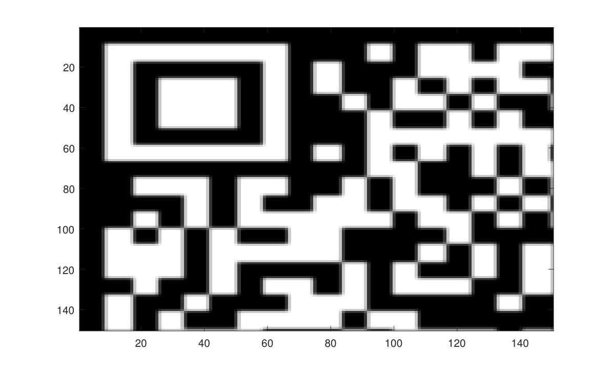 Figure 1
 Figure 2
 Figure 3
 Figure 4
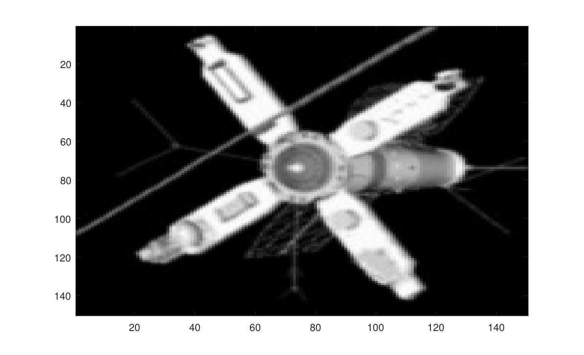 Figure 5
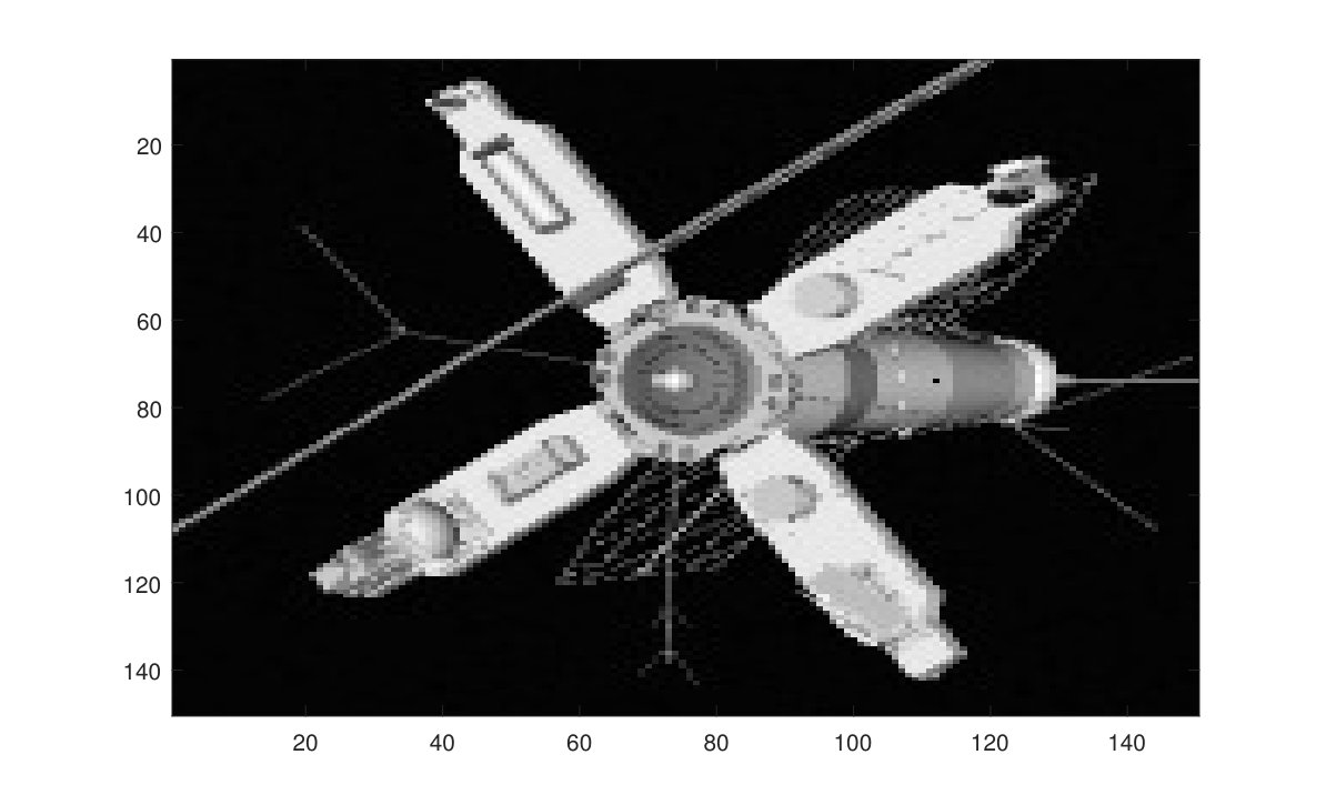 Figure 6
 Figure 7
 Figure 8
| regularization | number of | CPU time | relative |
|---|---|---|---|
| matrix | iterations | in seconds | error |
| noise level | |||
| regularization | number of | CPU time | relative |
|---|---|---|---|
| matrix | iterations | in seconds | error |
| noise level | |||
| noise level | |||
| noise level | |||
| regularization | number of | CPU time | relative |
|---|---|---|---|
| matrix | iterations | in seconds | error |
| noise level | |||
| noise level | |||
Peer Reviews
No public reviews on file for this paper yet. If you reviewed it on a platform where reviews are public (OpenReview, ICLR, NeurIPS, ICML), you can paste yours below so the community can read it here.
Videos
No videos yet. Explain this paper in a talk, walkthrough, or lecture? Add one.
Regularization matrices for discrete ill-posed problems in several
space-dimensions
Laura Dykes University School, Hunting Valley, OH 44022, USA. E-mail: [email protected].
Guangxin Huang Geomathematics Key Laboratory of Sichuan, College of Management Science, Chengdu University of Technology, Chengdu, 610059, P. R. China. E-mail: [email protected].
Silvia Noschese Department of Mathematics, SAPIENZA Università di Roma, P.le A. Moro, 2, I-00185 Roma, Italy. E-mail: [email protected].
Lothar Reichel Department of Mathematical Sciences, Kent State University, Kent, OH 44242, USA. E-mail: [email protected].
Abstract
Many applications in science and engineering require the solution of large linear discrete ill-posed problems that are obtained by the discretization of a Fredholm integral equation of the first kind in several space-dimensions. The matrix that defines these problems is very ill-conditioned and generally numerically singular, and the right-hand side, which represents measured data, typically is contaminated by measurement error. Straightforward solution of these problems generally is not meaningful due to severe error propagation. Tikhonov regularization seeks to alleviate this difficulty by replacing the given linear discrete ill-posed problem by a penalized least-squares problem, whose solution is less sensitive to the error in the right-hand side and to round-off errors introduced during the computations. This paper discusses the construction of penalty terms that are determined by solving a matrix-nearness problem. These penalty terms allow partial transformation to standard form of Tikhonov regularization problems that stem from the discretization of integral equations on a cube in several space-dimensions.
keywords:
Discrete ill-posed problems; Tikhonov regularization; standard form problems; matrix nearness problems; Krylov subspace iterative methods
AMS:
65F10; 65F22; 65R30
1 Introduction
We consider the solution of linear discrete ill-posed problems that arise from the discretization of a Fredholm integral equation of the first kind on a cube in two or more space-dimensions. Discretization of the integral operator yields a matrix , which we assume to be large. A vector \mbox{\boldmath{b}}\in{\mathbb{R}}^{M} that represents measured data, and therefore is error-contaminated, is available and we would like to compute an approximate solution of the least-square problem
[TABLE]
The matrix has many “tiny” singular values of different orders of magnitude. This makes severely ill-conditioned; in fact, may be numerically singular. Least-squares problems (1) with a matrix of this kind are commonly referred to as linear discrete ill-posed problems.
Let \mbox{\boldmath{e}}\in{\mathbb{R}}^{M} denote the (unknown) error in . Thus,
[TABLE]
where \widehat{\mbox{\boldmath{b}}}\in{\mathbb{R}}^{M} stands for the unknown error-free vector associated with . We will assume the unavailable linear system of equations
[TABLE]
to be consistent.
Let denote the Moore–Penrose pseudoinverse of the matrix . We are interested in determining the solution \widehat{\mbox{\boldmath{x}}} of (3) of minimal Euclidean norm; it is given by K^{\dagger}\widehat{\mbox{\boldmath{b}}}. We note that the solution of minimal Euclidean norm of (1),
[TABLE]
generally is not a meaningful approximation of \widehat{\mbox{\boldmath{x}}} due to a large propagated error K^{\dagger}\mbox{\boldmath{e}}. This difficulty stems from the fact that is large. Throughout this paper denotes the Euclidean vector norm or spectral matrix norm. We also will use the Frobenius norm of a matrix, defined by , where the superscript T stands for transposition.
To avoid severe error propagation, one replaces the least-squares problem (1) by a nearby problem, whose solution is less sensitive to the error in . This replacement is known as regularization. Tikhonov regularization, which is one of the most popular regularization methods, replaces (1) by a penalized least-squares problem of the form
[TABLE]
where is referred to as the regularization matrix and the scalar as the regularization parameter; see, e.g., [2, 8, 10]. We assume the matrix to be chosen so that
[TABLE]
where denotes the null space of the matrix . Then the minimization problem (4) has a unique solution
[TABLE]
for any .
Common choices of include the identity matrix and discretizations of differential operators. The Tikhonov minimization problem (4) is said to be in standard form when ; otherwise it is in general form. Numerous computed examples in the literature, see, e.g., [4, 5, 9, 25], illustrate that the choice of can be important for the quality of the computed approximation \mbox{\boldmath{x}}_{\mu} of \widehat{\mbox{\boldmath{x}}}. The regularization matrix should be chosen so that known important features of the desired solution \widehat{\mbox{\boldmath{x}}} of (3) are not damped. This can be achieved by choosing so that contains vectors that represent these features, because vectors in are not damped by .
Several approaches to construct regularization matrices with desirable properties are described in the literature; see, e.g., [1, 4, 5, 6, 12, 16, 19, 22, 23, 25, 27]. Huang et al. [16] propose the construction of square regularization matrices with a user-specified null space by solving a matrix nearness problem in the Frobenius norm. The regularization matrices so obtained are designed for linear discrete ill-posed problems in one space-dimension. This paper extends this approach to problems in higher space-dimensions. The regularization matrices of this paper generalize those applied by Bouhamidi and Jbilou [1] by allowing a user-specified null space.
Consider the special case of space-dimensions and let the matrix be determined by discretizing an integral equation on a square grid (i.e., ). The regularization matrix
[TABLE]
where is the identity matrix,
[TABLE]
and denotes the Kronecker product, has frequently been used for this kind of problem; see e.g., [3, 14, 19, 20, 26]. We note for future reference that .
It also may be attractive to replace the matrix (7) in (6) by
[TABLE]
with null space . This yields the regularization matrix
[TABLE]
Both the regularization matrices (6) and (9) are rectangular with almost twice as many rows as columns when is large.
Bouhamidi and Jbilou [1] proposed the use of the smaller invertible regularization matrix
[TABLE]
where
[TABLE]
is a square nonsingular regularization matrix. Therefore the regularization matrix (10) also is square and nonsingular, which makes it easy to transform the Tikhonov minimization problem (4) so obtained to standard form; see below.
Following Bouhamidi and Jbilou [1], we consider square matrices with a tensor product structure, i.e.,
[TABLE]
We assume for simplicity that with . However, we note that the regularization matrices described in this paper can be applied also when the matrix in (1) does not have a tensor product structure.
Bouhamidi and Jbilou [1] are concerned with applications to image restoration and achieve restorations of high quality. However, for linear discrete ill-posed problems in one space-dimension, analysis presented in [4, 12] indicates that the regularization matrix (8), with a non-trivial null space, can give approximate solutions of higher quality than the matrix (11), which has a trivial null space. This depends on that the latter matrix may introduce artifacts close to the boundary; see also [5, 6, 25] for related discussions and illustrations. It is the aim of the present paper to develop a generalization of the regularization matrix (9) that has a non-trivial null space. Our approach to define such a regularization matrix generalizes the technique proposed in [16] from one to several space-dimensions. Specifically, the regularization matrix is defined by solving a matrix nearness problem in the Frobenius norm. The regularization matrix so obtained allows a partial transformation of the Tikhonov regularization problem (4) to standard form. When the matrix is square, Arnoldi-type iterative solution methods can be used. Arnoldi-type iterative solution methods often require fewer matrix-vector product evaluations than iterative solution methods based on Golub–Kahan bidiagonalization, because they do not require matrix-vector product evaluations with ; see, e.g., [21] for illustrations. A nice recent survey of iterative solution methods for discrete ill-posed problems is provided by Gazzola et al. [9].
This paper is organized as follows. Section 2 describes our construction of new regularization matrices for problems in two space-dimensions. The section also discusses iterative methods for the solution of the Tikhonov minimization problems obtained. We consider both the situation when is a general matrix and when has a tensor product structure. Section 3 generalizes the results of Section 2 to more than two space-dimensions. Computed examples can be found in Section 4, and Section 5 contains concluding remarks.
We conclude this section by noting that while this paper focuses on iterative solution methods for large-scale Tikhonov minimization problems (4), the regularization matrices described also can be applied in direct solution methods for small to medium-sized problems that are based on the generalized singular value decomposition (GSVD); see, e.g., [7, 10] for discussions and references.
2 Regularization matrices for problems in two space-dimensions
Many image restoration problems as well as problems from certain other applications (1) have a matrix that is the Kronecker product of two matrices with , cf. (12). We will consider this situation in most of this section; the case when is a general square matrix without Kronecker product structure is commented on at the end of the section. Extension to rectangular matrices , , and is straightforward.
We will use regularization matrices with a Kronecker product structure,
[TABLE]
and will discuss the choice of square regularization matrices . The following result is an extension of [16, Proposition 2.1] to problems with a Kronecker product structure. Let denote the range of the matrix and define the Frobenius inner product
[TABLE]
between matrices . Throughout this section .
Proposition 1**.**
Let the matrices and have orthonormal columns, and let denote the subspace of matrices of the form , where the null space of contains for . Introduce for the orthogonal projectors with null space . Let . Then the matrix is a closest matrix to with , , in in the Frobenius norm.
Proof.
The matrix satisfies the following conditions:
; 2. 2.
if , then ; 3. 3.
if , then .
In fact,
[TABLE]
which shows the first property. The second property implies that
[TABLE]
from which it follows that
[TABLE]
Finally, for any of the form , one has that
[TABLE]
so that
[TABLE]
where the last equality follows from the cyclic property of the trace. ∎
Example 2.1. Let and be defined by (8) and (11), respectively. Proposition 1 shows that a closest matrix to in the Frobenius norm with null space is
[TABLE]
where is the orthogonal projector onto .
Example 2.2. Define the square nonsingular regularization matrix
[TABLE]
A closest matrix to in the Frobenius norm with null space is given by
[TABLE]
where is the orthogonal projector onto ; see, e.g., [16].
The following result is concerned with the situation when the order of the nonsingular matrices and projectors in Examples 2.1 and 2.2 is reversed. We first consider the situation when is a square matrix without Kronecker product structure, since this situation is of independent interest.
Proposition 2**.**
Let and let be a subspace of . Define the orthogonal projector onto . Then the closest matrix to in the Frobenius norm, such that , is given by .
Proof.
Consider the problem of determining a closest matrix to in the Frobenius norm whose null space contains . It is shown in [16, Proposition 2.3] that is such a matrix. The Frobenius norm is invariant under transposition and orthogonal projectors are symmetric. Therefore,
[TABLE]
Moreover, . It follows that a closest matrix to in the Frobenius norm whose range is a subset of is given by . ∎
The following result extends Proposition 2 to matrices with a tensor product structure. We formulate the result similarly as Proposition 1.
Corollary 3**.**
Let the matrices and have orthonormal columns, and let denote the subspace of matrices of the form , where the range of is orthogonal to for . Introduce for the orthogonal projectors and let . Then the matrix is a closest matrix to with , , in in the Frobenius norm.
Proof.
The result can be shown by applying Propositions 1 or 2. ∎
Example 2.3. Let be defined by (8) and by (11). Corollary 3 shows that a closest matrix to with range in is
[TABLE]
where .
Example 2.4. Let the matrices and be given by (7) and (15). It follows from Corollary 3 that a closest matrix to with range in is given by
[TABLE]
where .
Using (12) and (13), the Tikhonov regularization problem (4) can be expressed as
[TABLE]
It is convenient to introduce the operator , which transforms a matrix to a vector of size by stacking the columns of . Let , , and , be matrices of commensurate sizes. Then
[TABLE]
see, e.g., [15] for operations on matrices with Kronecker product structure. We can apply this identity to express (16) in the form
[TABLE]
where the matrix satisfies \mbox{\boldmath{b}}=\mathrm{vec}(B).
Let the regularization matrices in (17) be of the forms
[TABLE]
where the matrices are nonsingular and the are orthogonal projectors. We easily can transform (17) to a form with an orthogonal projector regularization matrix,
[TABLE]
where
[TABLE]
We will solve (19) by an iterative method. The structure of the minimization problem makes it convenient to apply an iterative method based on the global Arnoldi process, which was introduced and first analyzed by Jbilou et al. [17, 18]. We refer to matrices with many more rows than columns as “block vectors”. The block vectors are said to be -orthogonal if ; they are -orthonormal if in addition .
The application of steps of the global Arnoldi method to the solution of (19) yields an -orthonormal basis of block vectors for the block Krylov subspace
[TABLE]
In particular . The use of the global Arnoldi method to the solution of (19) is mathematically equivalent to applying a standard Arnoldi method to (16). An advantage of the global Arnoldi method is that it can be implemented by using matrix-matrix operations, while the standard Arnoldi method applies matrix-vector and vector-vector operations. This can lead to faster execution of the global Arnoldi method on many modern computers. Algorithm 1 outlines the global Arnoldi method; see [17, 18] for further discussions of this and other block methods.
We determine an approximate solution of (19) in the global Arnoldi subspace (20). This is described by Algorithm 2 for a given . The solution subspace (20) is independent of the orthogonal projectors that determine the regularization term in (19). This approach to generate a solution subspace for the solution of Tikhonov minimization problems in general form was first discussed in [13]; see also [9] for examples.
The discrepancy principle is a popular approach to determine the regularization parameter when a bound for the norm of the error in is known, i.e., \|\mbox{\boldmath{e}}\|\leq\varepsilon. It prescribes that be chosen so that the computed approximate solution of (19) satisfies
[TABLE]
where is a user-chosen constant independent of . The nonlinear equation (21) for can be solved by a variety of methods such as Newton’s method; see [13] for a discussion.
Finally, we note that the regularization matrices of this section also can be applied when the matrix in (4) does not have a Kronecker product structure (12). Let {\mbox{\boldmath{x}}}={\rm vec}(X). Then the matrix expression in the penalty term of (19) can be written as
[TABLE]
The analogue of the minimization problem (19) therefore can be expressed as
[TABLE]
The matrix is invertible; we have . It follows that the problem (22) can be transformed to
[TABLE]
The matrix is an orthogonal projector. It is described in [22] how Tikhonov regularization problems with a regularization term that is determined by an orthogonal projector with a low-dimensional null space easily can be transformed to standard form. However, , which generally is quite large in problems of interest to us. It is therefore impractical to transform the Tikhonov minimization problem (23) to standard form. We can solve (23), e.g., by generating a (standard) Krylov subspace determined by the matrix and vector , similarly as described in [13]. When the matrix is square, the Arnoldi process can be applied to generate a solution subspace; when is rectangular, partial Golub–Kahan bidiagonalization of can be used. The latter approach requires matrix-vector product evaluations with both and ; see [13] for further details.
3 Regularization matrices for problems in higher space-dimensions
Proposition 1 can be extended to higher space-dimensions. In addition to allowing space-dimensions, we remove the requirement that all blocks be square and of equal size.
Proposition 4**.**
Let have orthonormal columns for , and let denote the subspace of matrices of the form
[TABLE]
where the null space of contains for all . Let denote the identity matrix of order and define the orthogonal projectors
[TABLE]
Then the matrix is a closest matrix to in in the Frobenius norm, where , .
Proof.
The proof is a straightforward modification of the proof of Proposition 1. ∎
Let be a sequence of square nonsingular matrices, and let be regularization matrices with desirable null spaces. It follows from Proposition 4 that a closest matrix to
[TABLE]
with null space is
[TABLE]
where the orthogonal projectors are defined by (24) and the matrix has orthonormal columns that span for .
The following result generalizes Corollary 3 to higher space-dimensions and to rectangular blocks of different sizes.
Proposition 5**.**
Let have orthonormal columns for , and let denote the subspace of matrices of the form
[TABLE]
where the range of is orthogonal to for all . Let be defined by (24). Then the matrix is a closest matrix to in in the Frobenius norm, where , .
Proof.
The result can be shown by modifying the proof of Propositions 1 or 2. ∎
Let be a sequence of regularization matrices with desirable ranges, and let be full rank matrices. It follows from Proposition 5 that a closest matrix to
[TABLE]
with range in is
[TABLE]
where the orthogonal projectors are defined by (24) and the matrix has orthonormal columns that span for .
We conclude this section with an extension of (19) to higher space-dimensions and assume that the problem has a nested tensor structure, i.e.,
[TABLE]
where , , , and that
[TABLE]
where for . The minimization problem (1) with
[TABLE]
and \mbox{\boldmath{b}}=\mathrm{vec}(B) reads
[TABLE]
Let the regularization matrices have a nested tensor structure
[TABLE]
Then penalized least-squares problem that has to be solved is of the form
[TABLE]
If, moreover, the solution is separable of the form , where for , then we obtain the minimization problem
[TABLE]
When the regularization matrices are of the form , , where the are orthogonal projectors and the are square and invertible, the minimization problems (25) and (26) can be transformed similarly as equation (17) was transformed into (19).
4 Computed examples
We illustrate the performance of regularization matrices of the form with or for , and compare with the regularization matrices for . The noise level is given by
[TABLE]
Here is the error matrix, where is the available error-contaminated matrix in (17) and is the associated unknown error-free matrix, i.e., \widehat{\mbox{\boldmath{b}}}={\rm vec}(\widehat{B}); cf. (3). In all examples, the entries of the matrix are normally distributed with zero mean and are scaled to correspond to a specified noise level. We let in (21) in all examples. The quality of computed approximate solutions of (17) is measured with the relative error norm
[TABLE]
All computations were carried out in MATLAB R2017a with about significant decimal digits on a laptop computer with an Intel Core i7-6700HQ CPU @ 2.60GHz processor and 16GB RAM.
Example 4.1. Consider the Fredholm integral equation of the first kind in two space-dimensions,
[TABLE]
where . The kernel is given by
[TABLE]
where
[TABLE]
The right-hand side function is of the form
[TABLE]
where is chosen so that the solution is the sum of two Gaussian functions and a constant. We use the MATLAB code shaw from [11] to discretize (27) by a Galerkin method with orthonormal box functions as test and trial functions. This code produces the matrix that approximates the analogue of the integral operator (27) in one space-dimension, and a discrete approximate solution \mbox{\boldmath{x}}_{1} in one space-dimension. Adding the vector {\mbox{\boldmath{n}}}_{1}=[1,1,\ldots,1]^{T} yields the vector \widehat{\mbox{\boldmath{x}}}_{1}\in{{\mathbb{R}}}^{150}, from which we construct the scaled discrete approximation \widehat{X}=\widehat{\mbox{\boldmath{x}}}_{1}\widehat{\mbox{\boldmath{x}}}_{1}^{T} of the solution of (27). The error-free right-hand side is computed by . The error matrix models white Gaussian noise with noise levels and . The data matrix in (17) is computed as . The regularization matrices used are constructed like in Examples 2.1-2.4. We compare the performance of these regularization matrices to the performance of the nonsingular regularization matrices , , and . The number of steps, , of the global Arnoldi method is chosen as small as possible so that the discrepancy principle (21) can be satisfied. The regularization parameter is determined by the discrepancy principle.
Table 1 displays results obtained for the different regularization matrices and noise levels. The table shows the regularization matrices , , as well as to yield the smallest relative errors. Moreover, the computation with these regularization matrices requires the least CPU time. Figure 1 shows the computed approximate solution for the noise level when the regularization matrix is used. The computed approximation cannot be visually distinguished from the desired exact solution . We therefore do not show the latter.
Example 4.2. We consider the restoration of the test image satellite, which is represented by an array of pixels. The available image, represented by the matrix , is corrupted by Gaussian blur and additive zero-mean white Gaussian noise; it is shown in Figure 2(a). Figure 2(b) displays the desired blur- and noise-free image. It is represented by the matrix , and is assumed not to be known. The blurring matrices , , are Toeplitz matrices. We let , where is analogous to the matrix generated by the MATLAB function blur from [11] using the parameter values and . We show results for the noise levels , . The data matrix in (17) is determined similarly as in Example 4.1 and the regularization matrices used are the same as in Example 4.1.
Table 2 displays the number of iterations, CPU time, and the relative errors in the computed approximate solutions determined by the global Arnoldi process with data matrices contaminated by noise of levels , , for several regularization matrices. The iterations are terminated as soon as the discrepancy principle can be satisfied and the regularization parameter then is chosen so that (21) holds. Table 2 shows the global Arnoldi process with the regularization matrices , , and to yield the best approximations of and to require the least CPU time. Figures 2(c) and 2(d) show the computed approximate solutions determined by the global Arnoldi process with and the regularization matrices and , respectively. The quality of the computed restorations is visually indistinguishable.
Example 4.3. This example is similar to the previous one; only the image to be restored differs. Here we consider the restoration of the test image QRcode, which is represented by an array of pixels corrupted by Gaussian blur, and additive zero-mean white Gaussian noise. Figure 3(a) shows the corrupted image that we would like to restore. It is represented by the matrix . The desired blur- and noise-free image is depicted in Figure 3(b). The blurring matrices are Toeplitz matrices. They are generated like in Example 4.2. The regularization matrices are the same as in Example 4.2.
Table 3 is analogous to Table 2. The iterations are terminated as soon as the discrepancy principle (21) can be satisfied. The table shows the regularization matrices , , and to yield the most accurate approximations of . Figures 3(c) and 3(d) show the restorations determined for with the regularization matrices and , respectively. One cannot visually distinguish the quality of these restorations.
5 Concluding remarks
This paper presents a novel method to determine regularization matrices for discrete ill-posed problems in several space-dimensions by solving a matrix nearness problem. Numerical examples illustrate the effectiveness of the regularization matrices determined in this manner. While all examples use the discrepancy principle to determine a suitable value of the regularization parameter, other parameter choice rules also can be applied; see, e.g., [1, 24] for discussions and references.
Acknowledgment
Research by GH was supported in part by the Fund of Application Foundation of Science and Technology Department of the Sichuan Province (2016JY0249) and NNSF (11501392). Research by SN was partially supported by SAPIENZA Università di Roma and INdAM-GNCS.
The reference list from the paper itself. Each links out to its DOI / PubMed record.
- 1[1] A. Bouhamidi and K. Jbilou, Sylvester Tikhonov-regularization methods in image restoration , J. Comput. Appl. Math., 206 (2007), pp. 86–98.
- 2[2] C. Brezinski, M. Redivo–Zaglia, G. Rodriguez, and S. Seatzu, Extrapolation techniques for ill-conditioned linear systems , Numer. Math., 81 (1998), pp. 1–29.
- 3[3] D. Calvetti, B. Lewis, and L. Reichel, A hybrid GMRES and TV-norm based method for image restoration , in Advanced Signal Processing Algorithms, Architectures, and Implementations XII, ed. F. T. Luk, Proceedings of the Society of Photo-Optical Instrumentation Engineers (SPIE), vol. 4791, The International Society for Optical Engineering, Bellingham, WA, 2002, pp. 192–200.
- 4[4] D. Calvetti, L. Reichel, and A. Shuibi, Invertible smoothing preconditioners for linear discrete ill-posed problems , Appl. Numer. Math., 54 (2005), pp. 135–149.
- 5[5] M. Donatelli, A. Neuman, and L. Reichel, Square regularization matrices for large linear discrete ill-posed problems , Numer. Linear Algebra Appl., 19 (2012), pp. 896–913.
- 6[6] M. Donatelli and L. Reichel, Square smoothing regularization matrices with accurate boundary conditions , J. Comput. Appl. Math., 272 (2014), pp. 334–349.
- 7[7] L. Dykes, S. Noschese, and L. Reichel, Rescaling the GSVD with application to ill-posed problems , Numer. Algorithms, 68 (2015), pp. 531–545.
- 8[8] H. W. Engl, M. Hanke, and A. Neubauer, Regularization of Inverse Problems , Kluwer, Dordrecht, 1996.