A temporal Central Limit Theorem for real-valued cocycles over rotations
Michael Bromberg, Corinna Ulcigrai

TL;DR
This paper proves a Temporal Central Limit Theorem for deterministic random walks driven by irrational rotations with specific conditions, extending previous results to more general irrational parameters using renormalization and symbolic coding.
Contribution
It extends the Temporal CLT to irrational parameters using continued fraction and Ostrowski expansions, generalizing prior quadratic irrational cases.
Findings
Occupancy variables converge to Gaussian distribution
Extension of CLT to irrational skewing cocycles
Application of continued fraction renormalization
Abstract
We consider deterministic random walks on the real line driven by irrational rotations, or equivalently, skew product extensions of a rotation by where the skewing cocycle is a piecewise constant mean zero function with a jump by one at a point . When is badly approximable and is badly approximable with respect to , we prove a Temporal Central Limit theorem (in the terminology recently introduced by D.Dolgopyat and O.Sarig), namely we show that for any fixed initial point, the occupancy random variables, suitably rescaled, converge to a Gaussian random variable. This result generalizes and extends a theorem by J. Beck for the special case when is quadratic irrational, is rational and the initial point is the origin, recently reproved and then generalized to cover any initial point using geometric renormalization arguments by…
Click any figure to enlarge with its caption.
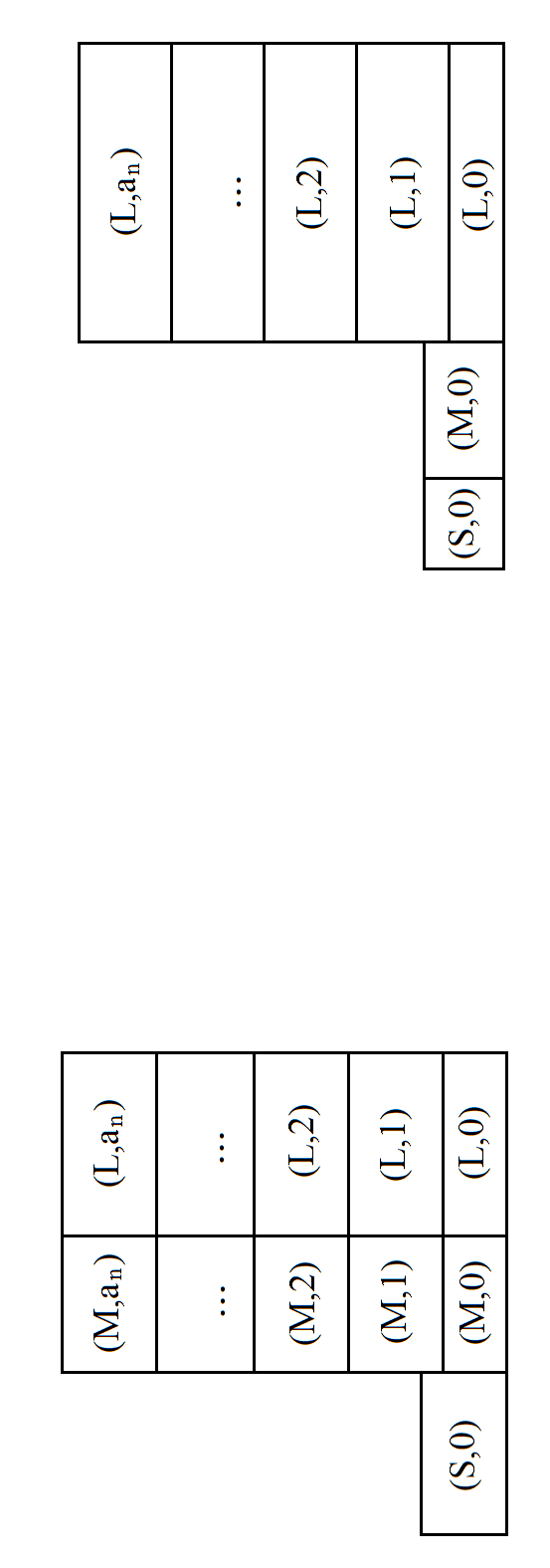 Figure 1
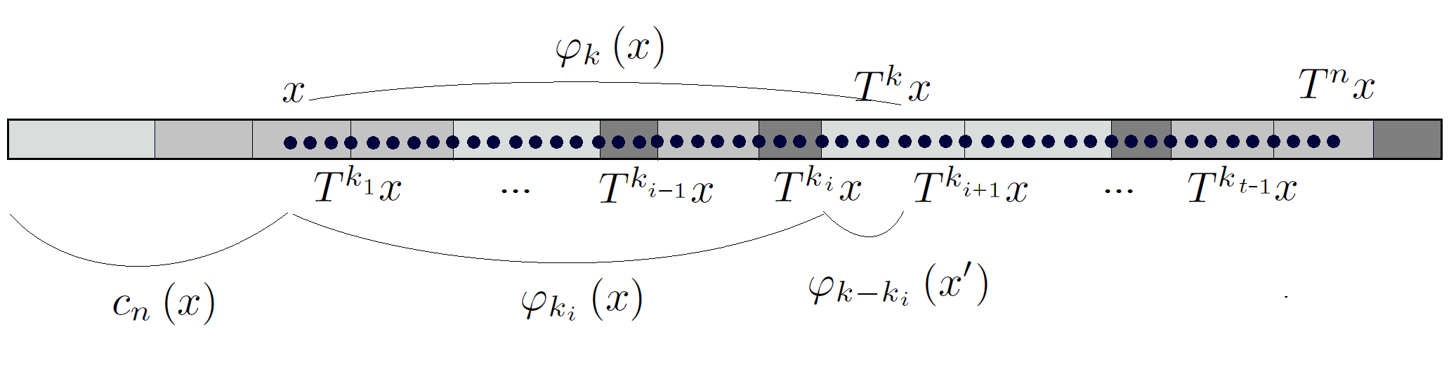 Figure 2
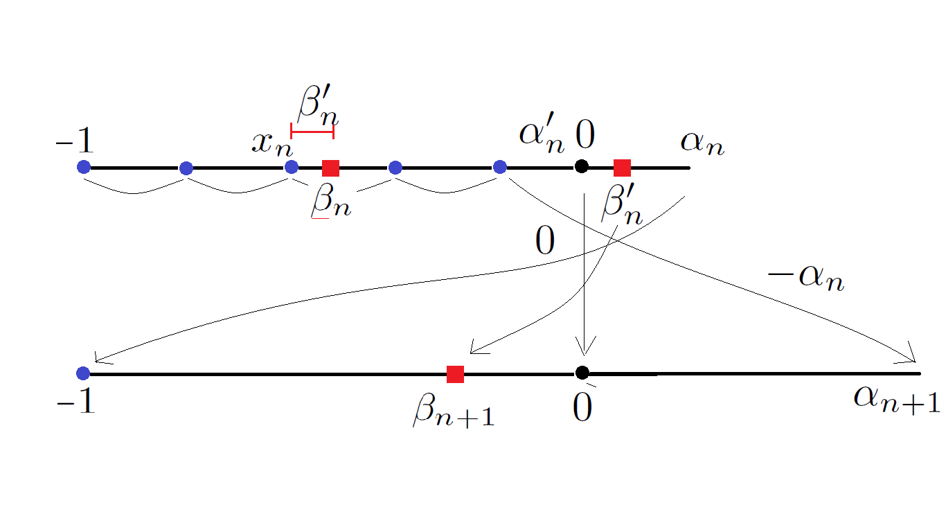 Figure 3
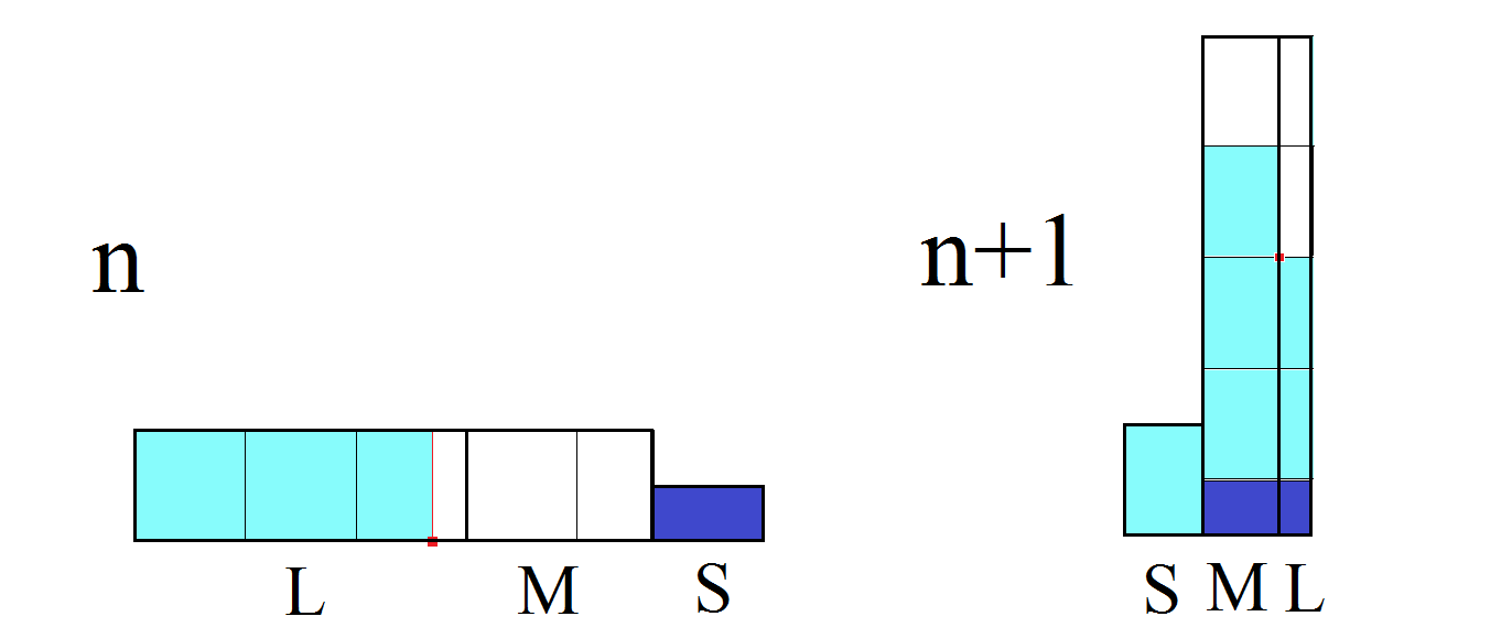 Figure 4
Peer Reviews
No public reviews on file for this paper yet. If you reviewed it on a platform where reviews are public (OpenReview, ICLR, NeurIPS, ICML), you can paste yours below so the community can read it here.
Videos
No videos yet. Explain this paper in a talk, walkthrough, or lecture? Add one.
A temporal Central Limit Theorem for real-valued cocycles over rotations
Michael Bromberg and Corinna Ulcigrai
Abstract.
We consider deterministic random walks on the real line driven by irrational rotations, or equivalently, skew product extensions of a rotation by where the skewing cocycle is a piecewise constant mean zero function with a jump by one at a point . When is badly approximable and** ** is badly approximable with respect to , we prove a *Temporal Central Limit theorem *(in the terminology recently introduced by D.Dolgopyat and O.Sarig), namely we show that for any fixed initial point, the occupancy random variables, suitably rescaled, converge to a Gaussian random variable. This result generalizes and extends a theorem by J. Beck for the special case when is quadratic irrational, is rational and the initial point is the origin, recently reproved and then generalized to cover any initial point using geometric renormalization arguments by Avila-Dolgopyat-Duryev-Sarig (Israel J., 2015) and Dolgopyat-Sarig (J. Stat. Physics, 2016). We also use renormalization, but in order to treat irrational values of , instead of geometric arguments, we use the renormalization associated to the continued fraction algorithm and dynamical Ostrowski expansions. This yields a suitable symbolic coding framework which allows us to reduce the main result to a CLT for non homogeneous Markov chains.
1. introduction and results
The main result of this article is a temporal distributional limit theorem (see Section 1.1 below) for certain functions over an irrational rotation (Theorem 1.1 below). In order to introduce and motivate this result, in the first section, we first define two types of distributional limit theorems in the study of dynamical systems, namely spatial and temporal. Temporal limit theorems in dynamics are the focus of the recent paper [19] by D. Dolgopyat and O. Sarig; we refer the interested reader to [19] and the references therein for a comprehensive introduction to the subject, as well as for a list of examples of dynamical systems known up to date to satisfy temporal distributional limit theorems. In section 1.2 we then focus on irrational rotations, which are one of the most basic examples of low complexity dynamical systems, and recall previous results on temporal limit theorems for rotations, in particular Beck’s temporal CLT. Our main result in stated in section 1.3, followed by a description of the structure of the rest of the paper in section 1.4.
1.1. Temporal and Spatial Limits in dynamics.
Distributional limit theorems appear often in the study of dynamical systems as follows. Let be a complete separable metric space, a Borel probability measure on and denote by is the Borel -algebra on . Let be a Borel measurable map. We call the quadruple a probability preserving dynamical system and assume that is ergodic with respect to . Let be a Borel measurable function and set
[TABLE]
We will also use the notation , or instead of , when it is clear from the context, what is the underlying transformation or function. The function is called (the ) Birkhoff sum (or also ergodic sum) of the function over the transformation . The study of Birkhoff sums, their growth and their behavior is one of the central themes in ergodic theory. When the transformation is ergodic with respect to by the Birkhoff ergodic theorem, for any , for -almost every , converges to as grows; equivalently, one can say that the random variables where is chosen randomly according to the measure , satisfy the strong law of large numbers. We will now introduce some limit theorems which allow to study the error term in the Birkhoff ergodic theorem.
The function is said to satisfy a spatial distributional limit theorem (spatial DLT) if there exists a random variable with no atoms , and sequences of constants , , such that the random variables , where is chosen randomly according to the measure , converge in distribution to . In this case we write
[TABLE]
It is the case that many *hyperbolic *dynamical systems, under some regularity conditions on , satisfy a spatial DLT with the limit being a Gaussian random variable. In the cases that we have in mind, the rate of mixing of the sequence of random variables is sufficiently fast, in order for them to satisfy the Central Limit Theorem (CLT). On the other hand, in many classical examples of dynamical systems with zero entropy, for which the random variables are highly correlated, the spatial DLT fails if is sufficiently regular. For example, this is the case when is an irrational rotation and is of bounded variation.
Perhaps surprisingly, many examples of dynamical systems with zero entropy satisfy a CLT when instead of averaging over the space , one considers the Birkhoff sums over a single orbit of some fixed initial condition . Fix an initial point and consider its orbit under . One can define a sequence of occupation measures on by
[TABLE]
for every Borel measurable . One can interpret the quantity as the fraction of time that the Birkhoff sums spend in the set , up to time . Let be a sequence of random variables distributed according to . We say that the pair satisfies a temporal distributional limit theorem (temporal DLT) along the orbit of , if there exists a random variable with no atoms , and two sequences and such that converges in distribution to . In other words, the pair satisfies a temporal DLT along the orbit of , if
[TABLE]
for every . If the limit is a Gaussian random variable, we call this type of behavior a temporal CLT along the orbit of . Note, that this type of result may be interpreted as convergence in distribution of a sequence of normalized random variables, obtained by considering the Birkhoff sums for and choosing randomly uniformly.
1.2. Beck’s temporal CLT and its generalizations
One example of occurrence of a temporal CLT in dynamical systems with zero entropy is the following result by Beck, generalizations of which are the main topic of this paper. Let us denote by the rotation on the interval by an irrational number , given by
[TABLE]
Let be the indicator of the interval where , rescaled to have mean zero with respect to the Lebesgue measure on , namely
[TABLE]
The sequence of random variables given by the Birkhoff sums , where is taken uniformly with respect to the Lebesgue measure, is sometimes referred to in the literature as the *deterministic random walk *driven by an irrational rotation (see for example [6]).
Beck proved [7, 8] that if is a quadratic irrational, and is rational, then the pair satisfies a temporal DLT along the orbit of . More precisely, he shows that there exist constants and such that for all ,
[TABLE]
Beck’s CLT relates to the theory of discrepancy in number theory as follows. If is irrational, by unique ergodicity of the rotation , the sequence of is equidistributed modulo one, i.e. in particular, for any** ** if we set
[TABLE]
then converges to , or, equivalently, . Discrepancy theory concerns the study of the error term in the expression . Beck’s result hence says that, when is a quadratic irrational and is* rational, *the error term , when is chosen uniformly in , can be normalized so that it converges to the standard Gaussian distribution as grows to infinity.
Let us also remark that the Birkhoff sums in the statement of Beck’s theorem are related to the dynamics of the map , defined by
[TABLE]
since one can see that the form of the iterates of is T_{f}^{n}\left(x,y\right)=\text{\left(R_{\alpha}^{n}\left(x\right),y+S_{n}\text{}\right).} This skew product map has been studied as one basic example in infinite ergodic theory and there is a long history of results on it, starting from ergodicity (see for example [30, 15, 3, 27, 6, 2]).
Recently, in [6], a new proof of Beck’s theorem for the special case where , which uses dynamical and geometrical renormalization tools. It is crucially based on the interpretation of the corresponding skew-product map as the Poincaré map of a flow on the staircase periodic surface, which was noticed and pointed out in [22]. In [19] this method is generalized to show that for any initial point , any quadratic irrational and any* rational* , there exists a sequence and a constant such that
[TABLE]
for all , . Dolgopyat and Sarig showed us how to use the staircase method to prove the temporal CLT also in the case when is badly approximable, for a.e. and (private communication), but their methods do not apply to the more general class of s that we treat in this paper. They also informed us that they can show that the temporal CLT does not hold for a.e. and .
1.3. Main result and comments
The main result of this paper is the following generalization of Beck’s temporal CLT, in which we consider certain irrational values of and badly approximable values of . Let us recall that is* badly approximable* (or equivalently, is of* bounded type*) if there exists a constant such that for any , . Equivalently, is badly approximable if the continued faction entries of are uniformly bounded. For let us say that is badly approximable with respect to if there exists a constant such that
[TABLE]
One can show that given a badly approximable , the set of which are badly approximable with respect to have full Hausdorff dimension.
Theorem 1.1**.**
Let be a badly approximable irrational number. For every badly approximable with respect to and every there exists a sequence of centralizing constants and a sequence of normalizing constants such that for all
[TABLE]
In other words, for every badly approximable, any badly approximable with respect to the pair satisfies the temporal CLT along the orbit of any . Note that the centralizing constants depend on , while the normalizing constants do not. We will see in Section 4.1 that badly approximable numbers with respect to can be explicitly described in terms of their Ostrowski expansion, using an adaptation of the continued fraction algorithm in the context of non homogenous Diophantine Approximation. Let us recall that quadratic irrationals are in particular badly approximable. Moreover, when* * is badly approximable, it follows from definition that any rational number is badly approximable with respect to . Thus, this theorem, already in the special case in which is assumed to be a quadratic irrational, since it includes irrational values of , gives a strict generalization of the results mentioned above. As we already pointed out, the temporal limit theorem, fails to hold for almost every value of . It would be interesting to see whether a temporal CLT holds for a larger class of values of .
While the proof of Theorem 1.1 was inspired and motivated by an insight of Dolgopyat and Sarig and based, as theirs, on renormalization, we stress that our renormalization scheme and the formalism that we develop is different. As remarked in the previous section, the proof of Beck’s theorem in [6, 19] exploits a geometric renormalization which is based on the link with the staircase flow and the existence of affine diffeomorphisms which renormalize certain directions of directional flows on this surface. This geometrical insight, unfortunately, as well as the interpretation of the map as the Poincaré map of a staricase flow, breaks down when is not rational. Our proof does not rely on this geometric picture, but uses only the more classical renormalization given by the continued fraction algorithm for rotations, with the additional information encoded by Ostrowski expansions in the context of non homogeneous Diophantine approximations (see Section 2). This renormalization allows to encode the dynamics symbolically and reduce it to the formalism of adic and Vershik maps [37]).
There is a large literature of results on limiting distributions for entropy zero dynamical systems, see for example [13, 14, 12, 18, 20, 35]. Let us mention two recent results in the context of substitution systems which are related to our work. Bressaud, Bufetov and Hubert proved in [11] a spatial CLT for substitutions with eigenvalues of modulus one along a subsequence of times. In the same context (substitutions with eigenvalues of modulus one), Paquette and Son [28] recently also proved a *temporal *CLT. In [1] a temporal CLT over quadratic irrational rotations and valued, piecewise constant functions with rational discontinuities, is shown to hold along subsequences.
While we wrote this paper specifically for deterministic random walks driven by rotations, there are other entropy zero dynamical systems where this formalism applies and for which one can prove temporal limit theorems using similar techniques. For example, in work in progress, we can prove temporal limit theorems also for certain linear flows on infinite translation surfaces and some cocycles over interval exchange transformation and more in general for certain adic systems (which are non-stationary generalizations of substitution systems, see [9]).
1.4. Proof tools and sketch and outline of the paper
In Section 2 we introduce the renormalization algorithm that we use, as a key tool in the proofs: this is essentially the classical multiplicative continued fraction algorithm, with additional data which records the relative position of the break point of the function under renormalization. This renormalization acts on the underlying parameter space to be defined in what follows, as a (skew-product) extension of the Gauss map, and it produces simultaneously the continued fraction expansion entries of and the Ostrowski expansion entries of . Variations on this skew product have been studied by several authors (see in particular [5, 33]) and it is well known that it is related to a section of the diagonal flow on the space of affine lattices (as explained in detail in [5]). In sections 2.4 and 2.5 we explain how the renormalization algorithm provides a way of encoding dynamics symbolically in terms of a Markov chain. More precisely, the dynamics of the map we are interested in translates in symbolic language to the adic or Vershik dynamics (on a Bratelli diagram given by the Markov chain), as explained in section. The original function defines under renormalization a sequence of induced functions (which correspond to Birkhoff sums of the function at first return times, called special Birkhoff sums in the terminology introduced by [25]). The Birkhoff sums of the function can be then decomposed into sums of special Birkhoff sums. This formalism and the symbolic coding allows to translate the study of the temporal visit distribution random variable to the study of a non-homogeneous Markov chain, see section 2.6. In Section 3 we provide sufficient conditions for a non-homogeneous Markov chain to satisfy the CLT. Finally, in Section 4 we prove that these conditions are satisfied for the Markov chain modeling the temporal distribution random variables.
2. renormalization
2.1. Preliminaries on continued fraction expansions and circle rotations
Let : be the Gauss map, given by , where denotes the fractional part. Recall that a regular continued fraction expansion of is given by
[TABLE]
where and =. In this case we write . Setting , , for , and , , for we have and
[TABLE]
Let , and be the irrational rotation given by. Then the Denjoy-Koksma inequality [21, 24] states that if is a function of bounded variation, then for any ,
[TABLE]
where is the variation of on .
In this section we define the dynamical renormalization algorithm we use in this paper, which is an extension of the classical continued fraction algorithm and hence of the Gauss map. This algorithm gives a dynamical interpretation of the notion of Ostrowski expansion of relative to in non-homogeneous Diophantine approximation. We mostly follow the conventions of the paper [5] by Arnoux and Fisher, in which the connection between this renormalization and homogeneous dynamics (in particular the geodesic flow on the space of lattices with a marked point, which is also known as the scenery flow) is highlighted. As in [5] we use a different convention for rotations on the circle. Let , and let be defined by
[TABLE]
Note that may also be viewed as a rotation on the circle where the equivalence relation on is given by . It is conjugate to the standard rotation on , where , by the map which maps the unit interval to the interval .
Remark 2.1*.*
In what follows, we slightly abuse notation by not distinguishing between the transformation and the transformation defined similarly on the interval by
[TABLE]
when viewed as transformations on the circle, and coincide.
Note that given an irrational rotation , we can assume without loss of generality that (otherwise consider the inverse rotation by ). If we set
[TABLE]
then for any and thus, apart from the first entry, the continued fraction entries of and coincide. If , are correspondingly the first entries in the expansion of and , then . Furthermore, given , let
[TABLE]
Then the mean zero with a discontinuity at , given by
[TABLE]
is the function that corresponds to the function in the introduction under the conjugation between and . Therefore, we are interested in the Birkhoff sums
[TABLE]
Henceforth, unless explicitly stated otherwise, we work with the transformation . The sequences , will correspond to the sequence of entries and the sequence of partial convergents in the continued fraction expansion of .
We denote by the Lebesgue measure on normalized to have total mass .
2.2. Continued fraction
renormalization and Ostrowski expansion
The renormalization procedure is an inductive procedure, where at each stage we induce the original transformation onto a subinterval of the interval we induced upon at the previous stage. We denote by the nested sequence of intervals which we induce upon, and by the first return map of onto . The nested sequence of intervals is chosen in such a way that the induced transformations are all irrational rotations. The next paragraph describes a step of induction given an irrational rotation on the interval defined by (2.2). The procedure is then iterated recursively by rescaling and performing the induction step once again. In general, we keep to the convention that we use as a superscript to denote objects related to the non-rescaled th step of renormalization, and as a subscript for the rescaled version.
One step of renormalization
For an irrational let , defined by the formula in (2.2) and . Then is an exchange of two intervals of lengths and respectively (namely and ). The renormalization step consists of inducing onto an interval , where is obtained by cutting a half-open interval of size from the left endpoint of the interval , i.e. , as many times as possible in order to obtain an interval of the from containing zero. More precisely, let
[TABLE]
so that contains exactly intervals of lengths plus an additional remainder of length (see Figure 2.1). If , let be such that belongs to the copy of the interval which is cut, otherwise set , i.e. define
[TABLE]
For , let us define to be the left endpoint of the copy of the interval which contains , otherwise, if , set ; let also , so that if then is the distance of from the left endpoint of the interval which contains it (Figure 2.1). In formulas
[TABLE]
Notice that and hence in particular it belongs to the segment of the orbit of [math] under .
Let and note that and that the induced transformation obtained as the first return map of on is again an exchange of two intervals, a short one and a long one . Hence, if we renormalize and *flip *the picture by multiplying by , the interval is mapped to , where
[TABLE]
and the transformation as first return on the interval is conjugated to . We then set
[TABLE]
so that Thus we have defined , and and completed the description of the step of induction.
Notice that by definition of and we have that
[TABLE]
and hence, by using equation (2.7), we get
[TABLE]
Repeating the described procedure inductively, one can prove by induction the assertions summarized in the next proposition.
Proposition 2.2**.**
Let where are defined inductively from by and set . Define a sequence of nested intervals , , by , and
[TABLE]
The induced map of on is conjugated to on the interval if is even or to on if is odd, where the conjugacy is given by , .
Let and let and be the sequences inductively111Note that given formulas (2.7) and (2.10) determine first and then, as function of and , also and hence . by the formulas (2.7) and (2.10). Then we have
[TABLE]
and the reminders are given by
[TABLE]
The expansion in (2.11) is an Ostrowski type expansion for in terms of . We call the integers the entries in the Ostrowski expansion of .
Remark 2.3*.*
Partial approximations in the Ostrowski expansions have the following dynamical interpretation. It well known that, for any , the finite segment of the orbit of [math] under (which can be thought of as a rotation on a circle) induce a partition of into intervals of two lengths (see for example [34]; these partitions correspond to the classical Rokhlin-Kakutani representation of a rotation as two towers over an induced rotation given by the Gauss map, see also Section 2.3 and Remark 2.6). The finite Ostrowski approximation gives one of the endpoints of the unique interval of this partition which contains (if it is the left or the right one depends on the parity as well as on whether is zero or not). In particular, we have that
[TABLE]
Remark 2.4*.*
Since the points are all in the orbit of the point [math] by the rotation , it follows from the correspondence between and that the Ostrowski expansion of appearing in the previous proposition is finite, i.e. for some if and only if . This condition is well known to be equivalent to the function (and hence also ) being a coboundary (see [29]) .
It follows from the description of the renormalization algorithm that
[TABLE]
where the function is defined by (2.10). The ergodic properties of a variation on the map
[TABLE]
were studied among others in [33].
Introduce the functions defined by
[TABLE]
The functions are defined so that the sequences and of continued fractions and Ostrowski entries are respectively given by , for any
By Remark 2.4, the restriction of the space to
[TABLE]
is invariant with respect to and we partition this space into three sets , defined by
[TABLE]
Explicitly, in terms of the relative position of , these sets are given by
[TABLE]
The reason for the choice of names , , for the thee parts of parameter space, which stand for Good () and Bad (), where Bad has two subcases, and (according to whether is positive or negative), will be made clear in Section 4.1.
2.3. Description of the Kakutani-Rokhlin
towers obtained from renormalization.
We assume throughout the present Section and Sections 2.4, 2.5 that we are given a fixed pair . The symbols used in this Section refer to the denominators of the convergent in the continued fraction expansion of , where is related to via (2.3).
The renormalization algorithm described above defines a nested sequence of intervals . We describe here below how the original transformation can be represented as a union of* towers* in a Kakutani skyscraper (the definition is given below) with base ; the tower structure of the skyscraper corresponding to the stage of renormalization is obtained from the towers of the previous skyscraper corresponding to the n stage by a cutting and stacking procedure. We will use these towers to describe what we call an* adic* symbolic coding of the interval (see section 2.4). In what follows, we give a detailed description of the tower structure and the coding.
Let us first recall that if a measurable set and a natural integer are such that the union is disjoint, we say that the union is a (dynamical) tower of base and height . The union can indeed be represented as a tower with floors, namely for so that acts by mapping each point in each level except the last one, to the point directly above it. A disjoint union of towers is called a skyscraper (see for example [26]). A subtower of a tower of base and height is a tower with the same height whose base is a subset.
As it was explained in the previous section, the induced map of on is an exchange of two intervals, a* long* and a* short* one. If is even, the long one is given by and the short one by . If is odd the long and short interval are respectively given by and . In both cases, these are the preimages of the intervals and under the conjugacy map given in Proposition 2.2. Notice also that , the non rescaled marked point corresponding to the point , further divides the two mentioned subintervals of into three, by cutting either the long or the short into two subintervals. We denote these three intervals and , where the letters , respectively correspond to middle (M), *long *(L) and short (S), and denotes the middle interval, while and denote (what is left of) the long one and the short one, after removing the middle interval. Explicitly, it is convenient to describe the intervals in terms of the partition , , defined in the end of the previous section. Thus, set
[TABLE]
We claim that the first return time of to the interval is constant on the subintervals , and . Moreover, the first return time over and equals to and respectively, while the first return time over equals either or , depending on whether or and hence on whether the middle interval was cut from the long or the short interval respectively. For , let us denote by the first return time of to under and let us denote by the tower with base and height .
Let us how describe how the tower structure at stage of the renormalization is related to the tower structure at stage . We will describe in detail as an example the particular case where is odd and (i.e. ), or equivalently (see also Figure 2.2). The other cases are summarized in Proposition 2.5 below. In the considered case, the heights of the three towers , at stage are given by for and . By the structure of the first return map , the intervals , partition the interval into intervals of equal length, and it follows that the first return time of is constant on and equals to
[TABLE]
It also follows that the tower over at stage is obtained by stacking the subtowers over the intervals on top of the tower (as shown in Figure 2.2). By construction, the point is obtained by vertically projecting the point from its location in the tower over down to the interval . According to our definitions, divides into and . As we have seen, the height of the towers at stage over the intervals and is the same and equals , but the composition of the towers is different. The tower is obtained by stacking, on top of the bottom tower , first subtowers of and then subtowers of on top of them; has a similar structure, with the tower in the bottom, but with subtowers of on top and then subtowers of stacked over (see Figure 2.2). The tower over remains unchanged, i.e .
It is convenient to describe the tower structure in the language of substitutions. Let us recall that a substitution on a finite alphabet is a map which associates to each letter of a finite word in the alphabet . To each with rational or linearly independent over , we associate a sequence of substitutions over the alphabet , where for ,
[TABLE]
if and only if the tower consists of subtowers of , stacked on top of each other in the specified order, i.e. the subtower of is stacked on top of . More formally,
[TABLE]
For example, in the case discussed above, since the tower is obtained by stacking, on top of each other, in order, , then subtowers of and then subtowers of , we have
[TABLE]
We will use the convention of writing for the block where the symbol is repeated times. With this convention, the above substitution can be written
If is a word where we will denote by the letter indexed by <. Using this notation, we can rewrite (2.16) as
[TABLE]
We summarize the tower structure and the associated sequence of substitutions in the following proposition. The substitution is determined by the location of , or equivalently, by the non-rescaled parameters and one can check that there are three separate cases corresponding to the parameters being in , or . One of the cases was analyzed in the discussion above, while the other cases can be deduced similarly, and the proof of the proposition is a straightforward induction on .
Proposition 2.5**.**
The first return time function of to is constant on each of the three intervals , . Thus, for ,
[TABLE]
where is the value of the first return time function on , which is given by
[TABLE]
The sequence of substitutions associated to the pair is given by the formulas, determined by the following cases
- •
If
[TABLE]
- •
If
[TABLE]
- •
If
[TABLE]
Remark 2.6*.*
It can be shown that due to irrationality of , the levels of the towers , form an increasing sequence of partitions that separates points and hence generates the Borel -algebra on (see for example [34]).
Let , , be the incidence matrix of the substitution with entries indexed by , where the entry indexed by , which we will denote by , gives the number of subtowers contained in among the subtowers of level which are stuck to form of tower . Equivalently, the entry gives the number of occurrences of the letter in the word . If we adopt the convention that the order of rows/columns of corresponds to , it follows from Proposition 2.5 that these matrices are then explicitly given by:
[TABLE]
[TABLE]
[TABLE]
In particular, if we denote by the column vector of heights towers, i.e. the transpose of , it satisfies the recursive relations
[TABLE]
Remark 2.7*.*
We remark briefly for the readers familiar with the Vershik adic map and the -adic formalism (even though it will play no role in the rest of this paper), that the sequence also allows to represent the map as a Vershik adic map. The associated Bratteli diagram is a non-stationary diagram, whose vertex sets are always indexed by with edges from to ; the ordering of the edges which enter the vertex at level is given exactly by the substitution word . We refer the interested reader to the works by Vershik [37] and to the paper by Berthe and Delecroix [9] for further information on Vershik maps, Brattelli diagrams and -adic formalism.
2.3.1. Special Birkhoff sums
Let us consider now the function defined by (2.5) which has a discontinuity at [math] and at . In order to study its Birkhoff sums (defined in (2.6)) , we will use the renormalization algorithm described in the previous section. Under the assumption that , determines a sequence of functions , where is a real valued function defined on obtained by inducing on , i.e. by setting
[TABLE]
The function is what Marmi-Moussa-Yoccoz in [25] started calling special Birkhoff sums: the value gives the Birkhoff sum of the function along the orbit of until its first return to , i.e. it represents the Birkhoff sum of the function along an orbit which goes from the bottom to the top of the tower .
One can see that since has mean zero and a discontinuity with a jump of at , its special Birkhoff sums , , again have mean zero and a discontinuity with a jump of . The points , , are defined in the renormalization procedure exactly so that has a jump of one at . Moreover, the function is constant on each level of the towers , , , and therefore, it is completely determined by a sequence of vectors
[TABLE]
where , for any . It then follows immediately from the towers recursive structure (see equation (2.16)) that the functions also satisfy the following recursive formulas given by the substitutions in Proposition 2.5:
[TABLE]
We finish this section with a few simple observations on the heights of the towers and on special Birkhoff sums along these towers that we will need for the proof of the main result. Let be the parameters associated to a given pair via the relations (2.3) and (2.4). Under the assumption that is badly approximable, since the heights of the towers appearing in the renormalization procedure satisfy ) and are bounded, there exists a constant such that
[TABLE]
It follows that for any , there exists a constant , such that if , then
[TABLE]
Moreover, by (2.1), the special Birkhoff are uniformly bounded, i.e.
[TABLE]
2.4. The (adic) symbolic coding
The renormalization algorithm and the formalism defined above lead to the symbolic coding of the dynamics of described in the present section. This coding is exploited in Section 2.5 to build an array of non-homogeneous Markov chains which models the dynamics.
Definition 2.8**.**
(Markov compactum) Let be a sequence of finite sets with and let be a sequence of matrices, such that is an matrix whose entries for any . The Markov compactum determined by is the space
[TABLE]
To describe the coding, recall that for each , each tower , where , is obtained by stacking at most *subtowers *of the towers (the type and order of the subtowers is completely determined by the word given by the substitution as described in Proposition 2.5). We will label these subtowers by , where the index satisfies and indexes the subtowers from bottom to top: more formally, is the label of the subtower of , with base , which is the subtower from the bottom (see Figure 2.3). Thus, for a fixed , denoting by the length of the word , the labels of the subtowers belong to
[TABLE]
When is the continued badly approximable, let be the largest of its continued fraction entries and consider the alphabet
[TABLE]
Remark 2.9*.*
It is not necessary for to be badly approximable in order for the construction of the present section and the next section to be valid. If is not badly approximable, define . This definition would make all statements of this and the following sections valid, without any further changes.
Definition 2.10**.**
Given , for each , is contained in a unique tower for some , and furthermore in a unique subtower of stage inside it, labeled by where . Let be the coding map defined by
[TABLE]
Let us recall that for word in the alphabet let us denote by the letter in the word which is labeled by 0\leq i<$$\left|\omega\right| .
Proposition 2.11**.**
The image of is contained in the subspace defined by
[TABLE]
The preimage under of any cylinder satisfying the constraints is the set of all points on some level of the tower , i.e. there exists such that
[TABLE]
Moreover, is a Borel isomorphism between and its image, where the Borel structure on the image of is inherited from the natural Borel structure on arising from the product topology on .
Let
[TABLE]
be the set of symbols which appear as coordinate in some admissible word in , and note that the definition of shows that is a Markov compactum with state space , given by a sequence of matrices indexed by such that if and only if . Although we do not need it in what follows, one can explicitly describe the image of the coding map and show that it is obtained from by removing countably many sequences. We remarked in Remark 2.7 that is conjugated to a the Vershik adic map. Let us add that the map provides the measure theoretical conjugacy.
Proof of Proposition 2.11.
First we prove that the image of is contained in . To see this, note that for , means that belongs to (since ) and means that belongs to the subtower of . Hence the subtower of must be contained in . Recalling the definition of the substitutions this implies exactly the relation , which in turn implies that .
To prove the second statement, namely that cylinders correspond to floors of towers, note that according to our labeling of the towers, the set of all such that consists exactly of all points which belong to levels of the tower , where . Proceeding by induction, one sees that for any , the set is the set of all points contained in precisely levels of the tower , where . Thus, since for any , is the set of all points on a single level of the tower . This argument shows that the levels of the towers , are in bijective correspondence under the map with cylinders of length in .
Finally, injectivity and bi-measurability of follow since the sequence of partitions induced by the tower structure generate the Borel sets of the space and separates points (see Remark 2.6). ∎
2.5. The Markov chain modeling towers.
In what follows, we denote by be the push forward by the map of the normalized Lebesgue measure on , i.e. the measure given by
[TABLE]
Moreover, for , let us define also the conditional measures
[TABLE]
We denote by and correspondingly, the restriction of and to the first coordinates and we endow these sets with the -algebras inherited from the Borel -algebra on . Let be the set of states appearing in the coordinate of , defined by (2.25).
We define a sequence of transition probabilities, or equivalently in this discrete case, stochastic matrices , where and , and a sequence of probability distributions on which are used to define a sequence of Markovian measures on that model the dynamical renormalization procedure. We refer to the sequence as the sequence of* transition matrices associated to the pair* .
Definition 2.12**.**
For any and , if
[TABLE]
we define
[TABLE]
[TABLE]
Moreover, for any , we set
[TABLE]
Remark 2.13*.*
The rationale behind the definition of is that is defined to be the - measure of the piece of the tower labeled by ; similarly is non zero exactly when the subtower inside is contained in , in which case it gives the proportion of this subtower which is contained in the subtower of labeled by .
The following Proposition identifies the measures and as Markovian measures on generated by the transition matrices and initial distributions indicated in the previous definition.
Proposition 2.14**.**
For every , and every word we have
[TABLE]
and
[TABLE]
Proof.
By Proposition 2.11, is non empty if and only if the sequence satisfies the conditions for , in which case it consists of the the set of all points on a certain level of the tower , i.e.
[TABLE]
It follows from the definition (2.26) of the measure that
[TABLE]
Moreover, we get that the conditional measures given by (2.27) satisfy
[TABLE]
Equations (2.28) now follow by definition of and which give that
[TABLE]
Hence, by the conditions for and recalling that and for any , we have that
[TABLE]
Equations (2.29) follows in the same way by using the definition of instead than .
Finally, if the sequence does not satisfy the conditions for , (by Proposition 2.11, as recalled above) and by definition of and , , we get that the right hand sides in (2.3) and (2.31) are both zero, so equations (2.3) and (2.31) hold in this case too. This completes the proof. ∎
For , , we define the *coordinate random variables *
[TABLE]
Since, all cylinders of the form , with generate the -algebra of , it immediately follows from Proposition 2.14 that for every , form a Markov chain on with respect to the measures , with transition probabilities , and initial distributions , , respectively.
2.6. The functions over the Markov chain modeling the Birkhoff sums.
Let us now define a sequence of functions that enables us to model the distribution of Birkhoff sums. In section 2.3.1 we introduced the notion of special Birkhoff sums of , i.e. Birkhoff sums of along the orbit of a point in the base of a renormalization tower up to the height of the tower, see (2.21). We will consider in this section intermediate Birkhoff sums along a tower (of for short, intermediate Birkhoff sums), namely Birkhoff sums of a point at the base of a tower up to an intermediate height, i.e. sums of the form
[TABLE]
The crucial Proposition (2.16) shows that intermediate Birkhoff sums can be expressed as sums of the following functions over the Markov chain .
Definition 2.15**.**
For , such that (note that this forces ), if set
[TABLE]
where, by convention, a sum with that runs from [math] to is equal to zero. If , set
[TABLE]
We then have the following proposition.
Proposition 2.16**.**
Let and let ,. Then for any ,
[TABLE]
Proof.
We show by induction on that, for any , any and , we have that
[TABLE]
where is the (unique) cylinder containing . To see this, note first that for , , and , we have and by definition of ,
[TABLE]
which proves the claim for . Now, assume that (2.31) holds for some . Then for , , and , let be the unique cylinder such that . Then and by Proposition 2.11 . It follows from definition of the map , that and
[TABLE]
Thus, setting , and using the definition of , we may write
[TABLE]
The previous equality is obtained by splitting the Birkhoff sum up to of a point at the base of the tower into special Birkhoff sums over towers obtained at the stage of the renormalization procedure and a remainder given by . Now, by definition of the coding map , . Thus, if for , we let denote the set , (2.32) implies,
[TABLE]
and the equality (2.31) now follows from the hypothesis of induction, which gives
[TABLE]
Since by Proposition 2.14, for any , and since by the proof of Proposition 2.11, the levels of the tower are in bijective correspondence with cylinders of length in , the proof is complete. ∎
3. the clt for markov chains
In the previous section we established that the study of intermediate Birkhoff sums can be reduced to the study of (in general) non-homogeneous Markov chains. In this section we establish some (mostly well-known) statements about such Markov chains which we use in the proof of our temporal CLT. The main result which we need is the CLT for non-homogeneous Markov chains. To the best of our knowledge, this was initially established by Dobrushin [16, 17] (see also [32] for a proof using martingale approximations). Dobrushin’s CLT is not directly valid in our case (since it assumes that the contraction coefficient is strictly less than for every transition matrix in the underlying chain, while under our assumptions this is only valid for a product of a constant number of matrices). While the proof of Dobrushin’s theorem can be reworked to apply to our assumptions, we do not do it here, and instead use a general CLT for -mixing triangular arrays of random variables by Utev.
3.1. Contraction coefficients, mixing properties and CLT for Markov chains
In this section we collect some probability theory results for (arrays of) non-homogeneous Markov chains that we will use in the next section.
Let be a probability space and let , be two sub -algebras of . For any -algebra , denote by the space of square integrable, real functions on , which are measurable with respect to . We use two measures of dependence between and , the so called -coefficient and -coefficient, defined by
[TABLE]
and
[TABLE]
It is a well-known fact (see [10]) that
[TABLE]
In what follows, let be a triangular array of mean zero, square integrable random variables such that the random variables in each row are defined on the same probability space . For any set of random variables defined on , let us denote by to be the -algebra generated by all the random variables in
Set and , . For any let
[TABLE]
[TABLE]
The array is said to be -mixing if as tends to infinity.
The following CLT for -mixing arrays of random variables, which follows from a more general CLT for such arrays in [36] is the main result that we use to prove our distributional CLT.
Theorem 3.1**.**
Let be a -mixing array of square integrable random variables and assume that
[TABLE]
for every . Then
[TABLE]
converges in law to the standard normal distribution.
Let be finite sets and a stochastic matrix with entries indexed by . The contraction coefficient of is defined by
[TABLE]
It is not difficult to see that if and only if the entry does not depend on and that
[TABLE]
for any pair of stochastic matrices and such that their product is defined.
For , let be a Markov chain with each taking values in a finite state space , determined by an initial distribution and transition matrices , (thus, each matrix has dimension ).
Proposition 3.2**.**
Assume that there exist and such that for every
[TABLE]
Then is -mixing and tends to [math] as with exponential rate.
Proof.
This is a direct consequence of the inequality
[TABLE]
(see relation (1.1.2) and Proposition 1.2.5 in [23]) and the fact that , which immediately follows from the assumption and (3.4). ∎
Now, let , with for any , be an array of functions and set . Henceforth, we assume that
[TABLE]
An application of Theorem 3.1 yields the following corollary.
Corollary 3.3**.**
Under the conditions of Proposition 3.2, assume further that and . Then converges in law to the standard normal distribution.
Proof.
It is enough to remark that the condition (3.2) in Theorem 3.1 holds trivially for large in virtue of the bound in (3.5) since by assumption the variance ∎
Let now be a sequence of probability distributions on , and let be an array of Markov chains generated by initial distributions and transition matrices . Let and let , .
Proposition 3.4**.**
Under the conditions of Proposition 3.2, there exists a constant , independent of the sequences and , such that and for all .
Proof.
The assumption implies that there exists a constant and a sequence of rank stochastic matrices (i.e stochastic matrices with all rows being identical) such that
[TABLE]
(see [31, Chapter 4, Cor. 2]), where for two matrices , indexed by , . Using (3.5) it follows that there exists a constant which depends only on the array of matrices and functions , such that
[TABLE]
Since the right hand side of the last inequality is a general term of a summable geometric series, we have proved that there exists a constant , such that for all .
To prove the inequality for the variances, we first note that it follows from (3.1) and (3.5) that there exists a constant independent of , such that
[TABLE]
for all . An analogous inequality hence holds also for the array instead of , so that
[TABLE]
Moreover, since , one can also prove that
[TABLE]
Now, write
[TABLE]
The proof of the Lemma hence follows by (3.7) and (3.8). ∎
4. proof of the temporal clt
In this section we give the proof of Theorem 1.1. We need to show that we can apply the results on Markov chains summarized in the previous section (and in particular Corollary 3.3) to the Markov chains that model the dynamics. In order to check that the required assumptions are verified, we first show, in section 4.1 a result on positivity of the product of finitely many transition matrices, which follows from the assumption that is badly approximable and is badly approximable with respect to . Then, in section 4.2 we prove that the variance grows. Finally, the proof of the Theorem is given in section 4.3.
4.1. Positivity of products of incidence
matrices
Let us recall that in Section 2.2 we described a renormalization procedure that, to a pair of parameters (under the assumption that ), in particular associates a sequence of matrices (given by equations (2.17), (2.18) and (2.19) respectively), which are the incidence matrices of the sequence of substitutions which describe the tower structure. In this section, we develop conditions on the pair that ensure that we may split the sequence of incidence matrices associated to into consecutive blocks of uniformly bounded length, so that the product of matrices in each block is strictly positive. This fact is used for showing that the Markov chain associated to satisfies the assumption of the previous section needed to prove the CLT.
Under the assumption that , the orbit of the point under the transformation defined in (2.13) is infinite and one can consider its* itinerary* with respect to the partition defined in Section 2.2: the itinerary is the sequence \left(s_{n}\right)_{n}\in\mathcal{S}^{\mathbb{N}\cup\text{\left{0\right} }}, where defined by
[TABLE]
We will call the set of states and we will say that s\left(\alpha,\beta\right):=\left(s_{n}\right)_{n}\in\mathcal{S}^{\mathbb{N}\cup\text{\left{0\right} }} the infinite sequence of states associated to . From the definitions in Section 2.2, (or respectively) if and only if the incidence matrix is of the form (2.17) (or (2.18), (2.19) respectively). It can be easily deduced from the description of the renormalization procedure that not all sequences in are images of some pair . The sequences s\in\mathcal{S}^{\mathbb{N}\cup\text{\left{0\right} }} such that for some ) form a stationary Markov compactum \tilde{\mathcal{S}}$$\subset\mathcal{S}^{\mathbb{N}\cup\text{\left{0\right} }} with state space determined by the graph,
[TABLE]
namely if and only if for any there is an oriented edge from the state to the state in the graph above.
Since at this point we are interested solely in positivity of the incidence matrices and not in the values themselves, we define a function , where are matrices, by
[TABLE]
Note that is defined in such a way, so that some entry of the matrix is , if and only if the corresponding entry of incidence matrix which corresponds to the state has a non-zero value, independently of and (for example and are always greater than or when ). Note that the other implication is not necessarily true, namely some entries of could be [math] even if the corresponding entry of the incidence matrices are positive (in such cases the positivity depends on the values of and , for example is zero if ). Thus, for any ,
[TABLE]
It immediately follows from the topology of the transition graph that every itinerary can be written in the form
[TABLE]
where , are words in the alphabet which do not contain (i.e. they are words in and , and is not empty for . Note that it may be that the number of appearances of in the above representation is finite. This means that there exists such that for and in this case the above representation reduces to
[TABLE]
where the length of is infinite.
Definition 4.1**.**
Let . We say that * is of Ostrowski bounded type with respect to* if the decomposition of given by (4.3) or (4.4) satisfies , where the supremum is taken over in the first case, and over in the second case. We say in both cases that * is of Ostrowski bounded type of order .*
Proposition 4.2**.**
Let be of Ostrowski bounded type of order with respect to and let bee i the sequence of incidence matrices associated to by the Ostrowski renormalization. Then for any , and any , we have that .
Proof.
Let the decomposition of described above. Direct calculation gives that the product of matrices which corresponds to an admissible word of length (or more) which does not contain is strictly positive. Also, any word of length which starts with gives a transition matrix which is strictly positive. Note that it follows from the transition graph that each , must start with and must be of length strictly greater than . Since any subword of length greater than must contain a block of the form , or a block of length at least where there is no occurrence of , the claim follows. ∎
Lemma 4.3**.**
If is badly approximable and is badly approximable with respect to , then the pair related to via equations (2.3) and (2.4), satisfies and is of Ostrowski bounded type with respect to .
Proof.
Let be the Ostrowski expansion of in terms of given by Proposition 2.2. Then by Remark 2.3 where are the denominators of the convergent in the continued fraction expansion of . Since under the conjugacy between and (where both maps are viewed as rotations on a circle), the (equivalence class of the) points [math] and in the domain of correspond respectively to the (equivalence class of) points and in the domain of , we obtain that . It follows that the Ostrowski expansion of is infinite, since otherwise, if there exists an such that , we would get that for some , which obviously contradicts (1.1). Thus, .
Fix and let be defined by (4.1). We claim that, if for some , for all , then there exist a constant , which does not depend on , and , , such that
[TABLE]
The second assertion of the Lemma follows immediately from this and the fact that as tends to .
To see that the claim holds, suppose that for all . Recalling the description of the renormalization procedure in section 2.2, this is equivalent to for all , so that. Thus, by the estimate of the reminder in an Ostrowski expansion given by Proposition 2.2, we obtain that
[TABLE]
Since is badly approximable, for all , where is a constant which depends only on . Since the conjugacy map is affine, the previous inequality yields that there exists a constant , such that
[TABLE]
Since , we obtain that
[TABLE]
where , and . Thus, combining the last two equations, we proved (4.5). This completes the proof of the Lemma. ∎
Let be badly approximable, let be badly approximable with respect to and let be related to via equations (2.3) and (2.4). Since by the previous proposition , the sequence of transition matrices associated to the pair given by Definition 2.12 is well defined. Recall that , where is a stochastic matrix, denotes the contraction coefficient defined by (3.3).
Corollary 4.4**.**
Let be badly approximable, be badly approximable with respect to and let be related to via equations (2.3) and (2.4). Then if is the sequence of transition matrices associated to (see Definition 2.12), there exist , and , such that
[TABLE]
Proof.
Lemma 4.3 implies that is of Ostrowski bounded type. By definition of the transition matrices (see Definition 2.12), for any ,
[TABLE]
if and only if
[TABLE]
This should be interpreted as the statement that the probability to pass from a state to some state is positive if and only if the intersection of the tower with the subtower of labelled by is non-empty. Thus, Proposition 4.2 implies that there exists such that is strictly positive for any . From being badly approximable (see inequality (2.23)) and by the fact that by definition, every positive entry of is a ratio between the heights of tower at the and stage of the renormalization, it follows that there exists which is independent of , such that every entry of is not less than . Note that it follows from the definition of the coefficient (see (3.3)) that if is a stochastic matrix such that there exists , for which , for all , , then . Thus, the proof is complete. ∎
4.2. Growth of the variance
In this section we consider the random variables , constructed in Section 2.6 (see equation (2.30) therein). Recall that the array is well defined for any given pair of parameters and, by the key Proposition 2.16, models Birkhoff sums over the transformation of the function defined by (2.5), which has a jump at . The goal in the present section is to show that if is not a coboundary, then the variance tends to infinity as tends to infinity, where is the variance of with respect to the measure .
Let us first recall the definition of tightness and a criterion which characterizes coboundaries.
Definition 4.5**.**
Let be a probability space. A sequence of random variables defined on and taking values in a Polish space is tight if for every , there exists a compact set such that , .
Let be a probability preserving system and let be a measurable function. We say that is a coboundary if there exists a measurable function such that the equality holds almost surely. Let us recall the following characterization of coboundaries on (see [4]).
Theorem 4.6**.**
The sequence is tight if and only if is a coboundary.
Set , . We will now prove the following lemma.
Lemma 4.7**.**
Assume that there exists a strictly increasing sequence of positive integers such that
[TABLE]
Then the sequence is tight.
Thus, combining Theorem 4.6 and Lemma 4.7 we have the following.
Corollary 4.8**.**
If does not tend to infinity as , then must be a coboundary.
Proof of Lemma 4.7..
Fix . By Markov’s inequality the assumption that , implies that there exists a constant such that for every ,
[TABLE]
Let and fix such that for any (this is possible since the heights of the towers tend to infinity with ). Let be any point on level of the tower and consider the Birkhoff sums . Then there exists a point in the base of the tower such that . Since the values of for and do not depend on we can choose any point and by triangle inequality we have that implies that or for any point on level of the tower with . Thus,
[TABLE]
where the last inequality follows by using that and recalling that by choice of we have that . Furthermore, by a change of indexes,
[TABLE]
where the last equality follows from Proposition 2.16. Therefore, from the relation between the measures and (see Definition 2.12) it follows that
[TABLE]
It follows from (4.6) that . Since was chosen arbitrarily, this shows that is tight. ∎
4.3. Proof of Theorem 1.1.
We begin this section with a few observations that summarize the results obtained in the preceding sections in the form that is used in order to prove Theorem 4.9 below from which the main theorem follows.
Let be badly approximable and be badly approximable with respect to . By Lemma 4.3 the pair related to via equations (2.3) and (2.4), satisfies . To each such pair, in Section 2.5 we associated a Markov compactum given by a sequence of transition matrices (which are incidence matrices for the substitutions which describe the Rokhlin tower structure) and Markov measures with transition matrices (defined in 2.26 and Definition 2.12 respectively). Let be the coordinate functions on the Markov compactum (see 2.30) and be the functions also defined therein (see Definition 2.15), which can be used to study the behavior of Birkhoff sums of the function defined by (2.5) over in virtue of as proved in Proposition 2.16. We set
[TABLE]
where the subscript in and mean that all integrals are taken with respect to the measure .
Since the function defined by (2.5) is not a coboundary (see Remark 2.4), Corollary 4.8 implies that . By definition of , combining the assumption that is badly approximable with the inequality (2.24), we obtain that
[TABLE]
Finally, for any , set , , for . Let us then define a Markov array , where for every set in the Borel -algebra of the space . The observations above together with Corollary 4.4 show that all assumptions of Corollary 3.3 hold for this array. Thus
[TABLE]
Moreover, by Proposition 3.4 (and the fact the ), (4.7) holds with replaced by , for any (where are the conditional measures defined by (2.27)).
We can now deduce the temporal CLT for Birkhoff sums. Fix . Let us first define the centralizing and normalizing constants for the Birkhoff sums For , let . Let be the tower at stage of the renormalization which contains the point and let be the level of the tower which contains , i.e. satisfies . Set where is any point in , i.e. is the Birkhoff sum over the tower from the bottom of the tower and up to the level that contains .
We will prove the following temporal DLT, from which Theorem 1.1 follows immediately recalling the correspondence between and and the functions and (refer to the beginning of Section (2.2)).
Theorem 4.9**.**
For any ,
[TABLE]
The above formulation, in particular, shows that the centralizing constants depend on the point and have a very clear dynamical meaning. The proof of this Theorem, which will take the rest of the section, is based on a quite standard decomposition of a Birkhoff sums into special Birkhoff sums. For each intermediate Birkhoff sum along a tower, we then exploit the connection with the Markov chain given by Proposition 2.16 and the convergence given by (4.7).
Proof.
Fix , , and let . By definition of , the points are contained in at most two towers obtained at the level of the renormalization. Let be defined by . Evidently, , and by (2.22) there exists which depends on but not on , such that .
Thus, since towers of level are decomposed into towers of level we can decompose the orbit into blocks which are each contained in a tower of level . More precisely, as shown in Figure (4.1), there exist and towers appearing at the stage of renormalization, such that for . Moreover, for , the set contains exactly points, i.e. and the points , belong to the level of the tower . Since the orbit segment is contained in at most two towers of level and each tower of level contains at most towers of level , we have that and hence is uniformly bounded in .
It follows from this decomposition that, for any interval ,
[TABLE]
where the last inequality follows from the fact that and are both not greater than . Evidently, we also have the opposite inequality
[TABLE]
For , and , write
[TABLE]
where is any point in .
By definition of , where belongs to the base (see Figure 4.1), thus is a sum of special Birkhoff sums over subtowers of , . Hence,
[TABLE]
by (2.24), there exists a constant which does not depend on , such that . It follows from Proposition 2.16 that
[TABLE]
Since , we have that and . Moreover, since , it follows from (4.7), that for any
[TABLE]
Let be such that for all and any ,
[TABLE]
Then if , by (4.8) and (4.10), recalling that ,
[TABLE]
Similarly, by (4.9), if , using this time that , we obtain the lower bound
[TABLE]
This completes the proof. ∎
Acknowledgments.
We would like to thank Jon Aaronson, Dima Dolgopyat, Jens Marklof and Omri Sarig for useful discussions and for their interest in our work. Both authors are supported by the ERC Starting Grant ChaParDyn. C. U. is also supported by the Leverhulm Trust through a Leverhulme Prize. The research leading to these results has received funding from the European Research Council under the European Union Seventh Framework Programme (FP/2007-2013) / ERC Grant Agreement n. 335989.
The reference list from the paper itself. Each links out to its DOI / PubMed record.
- 1[1] Jon Aaronson, Michael Bromberg, and Nishant Chandgotia. Rational ergodicity of step function skew products. ar Xiv preprint ar Xiv:1703.09003 , 2017.
- 2[2] Jon Aaronson, Michael Bromberg, and Hitoshi Nakada. Discrepancy skew products and affine random walks. ar Xiv preprint ar Xiv:1603.07233 , 2016.
- 3[3] Jon Aaronson and Michael Keane. The visitors to zero of some deterministic random walks. Proceedings of the London Mathematical Society , 3(3):535–553, 1982.
- 4[4] Jon Aaronson and Benjamin@articlepetersen 1973 series, title=On a series of cosecants related to a problem in ergodic theory, author=Petersen, Karl, journal=Compositio Mathematica, volume=26, number=3, pages=313–317, year=1973 Weiss. Remarks on the tightness of cocycles. In Colloq. Math , volume 84, pages 363–376, 2000.
- 5[5] Pierre Arnoux and Albert M Fisher. The scenery flow for geometric structures on the torus: the linear setting. Chinese Annals of Mathematics , 22(04):427–470, 2001.
- 6[6] Artur Avila, Dmitry Dolgopyat, Eduard Duryev, and Omri Sarig. The visits to zero of a random walk driven by an irrational rotation. Israel Journal of Mathematics , 207(2):653–717, 2015.
- 7[7] József Beck. Randomness of the square root of 2 and the giant leap, part 1. Periodica Mathematica Hungarica , 60(2):137–242, 2010.
- 8[8] József Beck. Randomness of the square root of 2 and the giant leap, part 2. Periodica Mathematica Hungarica , 62(2):127–246, 2011.