Minimally subtracted six loop renormalization of $O(n)$-symmetric $\phi^4$ theory and critical exponents
Mikhail V. Kompaniets, Erik Panzer

TL;DR
This paper computes high-order perturbative renormalization group functions for $O(n)$-symmetric $ ^4$ theory, providing precise estimates of critical exponents in lower dimensions through advanced loop calculations and resummation techniques.
Contribution
It presents the sixth loop order renormalization functions and estimates for critical exponents, extending previous calculations to higher loops and including non-subdivergent diagrams up to 11 loops.
Findings
Sixth loop order renormalization group functions computed.
Critical exponents estimated in three and two dimensions.
Comparison of asymptotic beta function behaviour with diagram estimates.
Abstract
We present the perturbative renormalization group functions of -symmetric theory in dimensions to the sixth loop order in the minimal subtraction scheme. In addition, we estimate diagrams without subdivergences up to 11 loops and compare these results with the asymptotic behaviour of the beta function. Furthermore, we perform a resummation to obtain estimates for critical exponents in three and two dimensions.
Click any figure to enlarge with its caption.
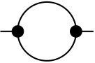 Figure 1
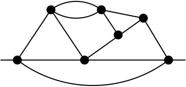 Figure 2
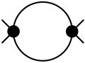 Figure 3
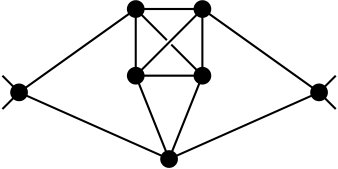 Figure 4
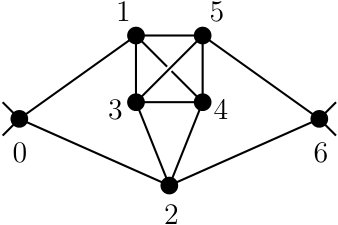 Figure 5
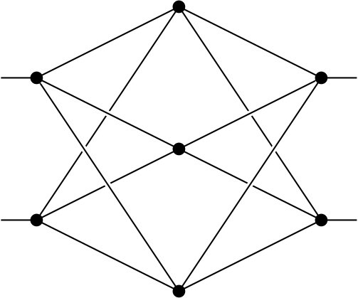 Figure 6
 Figure 7
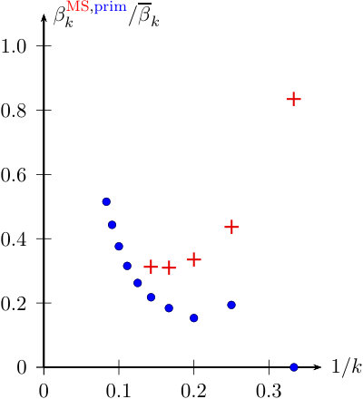 Figure 8
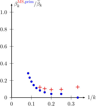 Figure 9
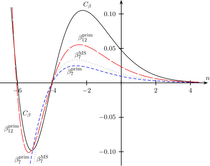 Figure 10
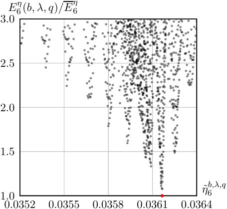 Figure 11
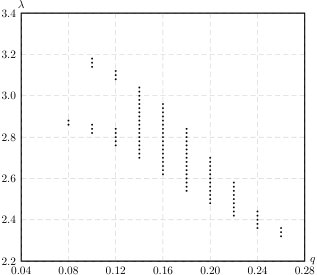 Figure 12
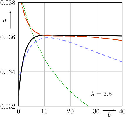 Figure 13
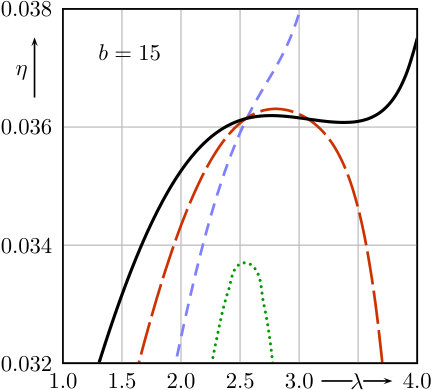 Figure 14
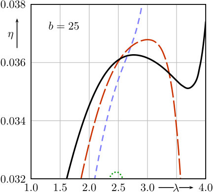 Figure 15
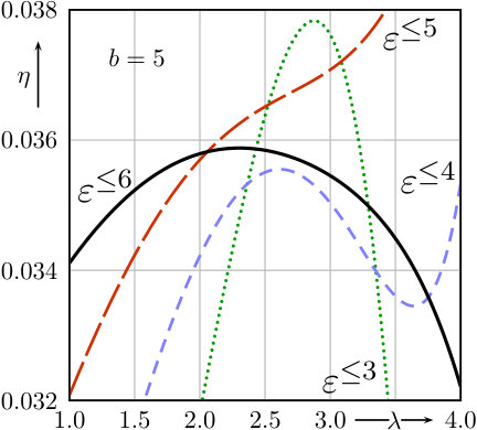 Figure 16
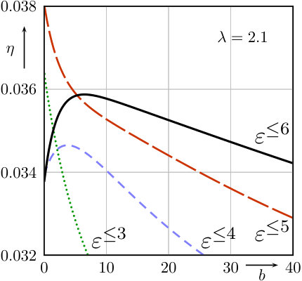 Figure 17
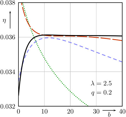 Figure 18
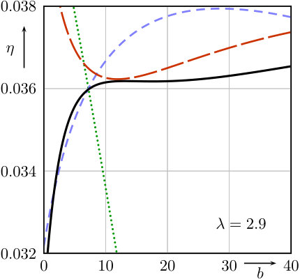 Figure 19
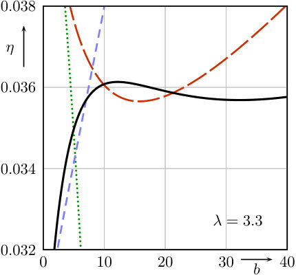 Figure 20
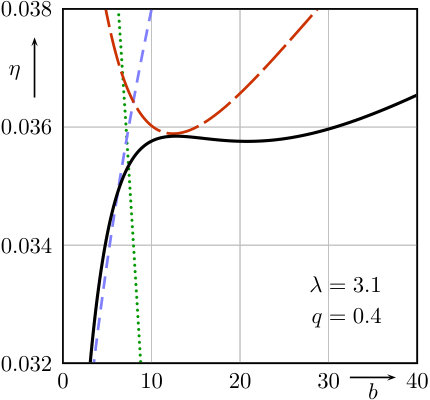 Figure 21
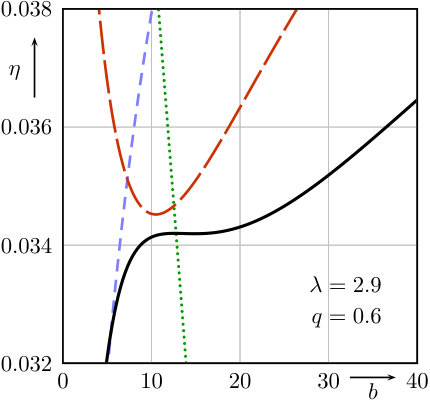 Figure 22
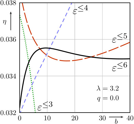 Figure 23
 Figure 24
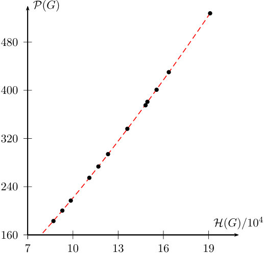 Figure 25
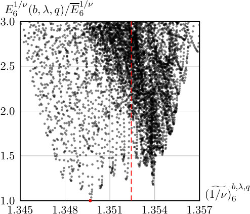 Figure 26
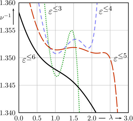 Figure 27
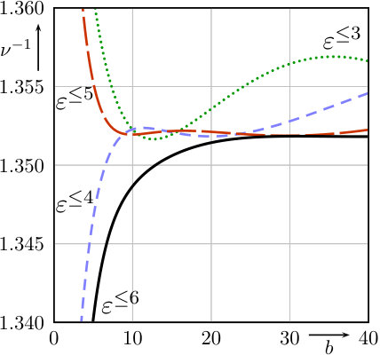 Figure 28
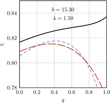 Figure 29
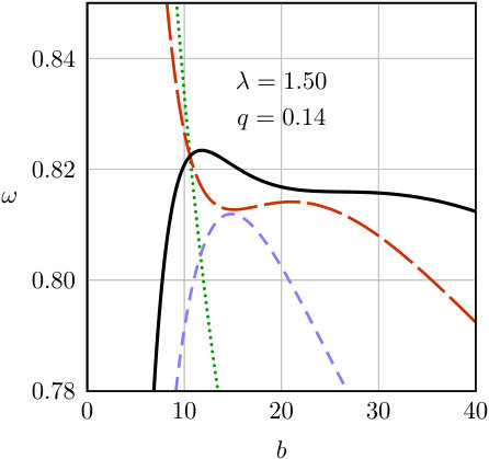 Figure 30
| loops | 1 | 2 | 3 | 4 | 5 | 6 | 7 |
|---|---|---|---|---|---|---|---|
| 2-point graphs () | 0 | 1 | 1 | 4 | 11 | 50 | 209 |
| 4-point graphs () | 1 | 2 | 8 | 26 | 124 | 627 | 3794 |
| primitive 4-point graphs () | 1 | 0 | 1 | 1 | 3 | 10 | 44 |
| 0 | 1 | 2 | 3 | 4 | 5 | |
| 23315 | 34776 | 48999 | 66243 | 86768 | 110840 | |
| APAP EllisKarlinerSamuel:betaQCDprediction | 23656 | 35374 | 49916 | 67604 | 88660 | |
| error | 1.46% | 1.72% | 1.87% | 2.06 % | 2.18% | |
| APAP ChishtieEliasSteele:MassivePhi4 | 35233 | 49381 | 66426 | 86636 | 110292 | |
| error | 1.31% | 0.78% | 0.28% | -0.15% | -0.50% | |
| 1355 | 2434 | 3950 | 5983 | 8618 | ||
| APAP ChishtieEliasSteele:MassivePhi4 | 1478 | 2740 | 4803 | 9476 | -3374 | |
| error | 9% | 13% | 22% | 58% | -139% | |
| 14.4 | 24.7 | 38.4 | 55.9 | 77.5 | ||
| APAP ChishtieEliasSteele:MassivePhi4 | 11.2 | 20.7 | 35.0 | 56.2 | 87.3 | |
| error | -22.0% | -16.3% | -8.9% | 0.5% | 12.6% |
| loop order | 1 | 2 | 3 | 4 | 5 | 6 |
|---|---|---|---|---|---|---|
| in % | 548 | 83.5 | 43.8 | 33.5 | 30.9 | 31.4 |
| in % | 43.1 | 12.5 | 9.58 | 9.41 | 10.4 | 12.1 |
| 3 | 5.67 | 32.5 | 272 | 2849 | 34776 | |
| 3 | 0 | 14.4 | 124 | 1698 | 24130 | |
| in % | 100 | 0 | 44.3 | 45.8 | 59.6 | 69.4 |
| loop order | first zero | second zero | third zero | |
|---|---|---|---|---|
| \ldelim{6*[] | 1 | -8 | ||
| 2 | -4.67 | |||
| 3 | -4.025 | -41.4 | ||
| 4 | -4.020 | -12.1 | 3219 | |
| 5 | -4.0017 | -8.76 | -44.0 | |
| 6 | -4.00044 | -7.52 | -20.0 | |
| \ldelim{6*[] | 6 | -3.99754 | -7.22 | -35.6 |
| 7 | -3.99982 | -6.58 | -15.1 | |
| 8 | -3.99994 | -6.31 | -10.8 | |
| 9 | -3.999997 | -6.18 | -9.24 | |
| 10 | -3.99999991 | -6.10 | -8.55 | |
| 11 | -4.000000095 | -6.05 | -8.21 |
| \ldelim{4*[] | 0.031043(3)191919From Clisby:ScaleFreeSAW and ClisbyDuenweg:Hydrodynamic via in (10). | 0.036298(2)KosPolandDuffinVichi:Islands | 0.0381(2)CampostriniHasenbuschPelissettoVicari:4He | 0.0378(3)HasenbuschVicari:Anisotropic | 0.0360(3)202020Given in HasenbuschVicari:Anisotropic and compatible with Hasenbusch:EliminatingN34 and in Deng:O(4) . | |
|---|---|---|---|---|---|---|
| 0.0310(7) | 0.0362(6) | 0.0380(6) | 0.0378(5) | 0.0366(4) | ||
| 0.0314(11) | 0.0366(11) | 0.0384(10) | 0.0382(10) | 0.0370(9) | ||
| GuidaZinnJustin:CriticalON | 0.0300(50) | 0.0360(50) | 0.0380(50) | 0.0375(45) | 0.036(4) | |
| \ldelim{4*[] | 0.5875970(4)ClisbyDuenweg:Hydrodynamic | 0.629971(4)KosPolandDuffinVichi:Islands | 0.6717(1)CampostriniHasenbuschPelissettoVicari:4He | 0.7112(5)CampostriniHasenbuschPelissettoRossiVicari:Heisenberg | 0.7477(8)212121From in Deng:O(4) , compatible with Hasenbusch:EliminatingN34 and HasenbuschVicari:Anisotropic . | |
| 0.5874(3) | 0.6292(5) | 0.6690(10) | 0.7059(20) | 0.7397(35) | ||
| 0.5873(13) | 0.6290(20) | 0.6687(13) | 0.7056(16) | 0.7389(24) | ||
| GuidaZinnJustin:CriticalON | 0.5875(25) | 0.6290(25) | 0.6680(35) | 0.7045(55) | 0.737(8) | |
| \ldelim{4*[] | 0.904(5)222222Computed from according to Belohorec:PhD and in ClisbyDuenweg:Hydrodynamic . | 0.830(2)3dIsingBootstrapII | 0.811(10)e | 0.791(22)e | 0.817(30)232323These are the results given as in (EcheverriHarlingSerone:EffectiveBootstrap, , Table 2). | |
| 0.841(13) | 0.820(7) | 0.804(3) | 0.795(7) | 0.794(9) | ||
| 0.835(11) | 0.818(8) | 0.803(6) | 0.797(7) | 0.795(6) | ||
| GuidaZinnJustin:CriticalON | 0.828(23) | 0.814(18) | 0.802(18) | 0.794(18) | 0.795(30) |
| \ldelim{4*[] | Nienhuis:ExactO(n) | |||
|---|---|---|---|---|
| 0.130(17) | 0.201(25) | 0.237(27) | ||
| 0.137(23) | 0.215(35) | 0.249(38) | ||
| GuillouZinnJustin:Accurate | 0.21(5) | 0.26(5) | ||
| \ldelim{4*[] | Nienhuis:ExactO(n) | |||
| 0.6036(23) | 0.741(4) | 0.952(14) | ||
| 0.6025(27) | 0.747(20) | 0.944(48) | ||
| GuillouZinnJustin:Accurate | 0.76(3) | 0.99(4) | ||
| \ldelim{4*[] | 2Nienhuis:ExactO(n) ; CGJPRS:Scaling2dSAW | 1.75CalabreseCaselleCeliPelissettoVicari:NonAnalyticity | ||
| 1.95(28) | 1.90(25) | 1.71(9) | ||
| 1.88(30) | 1.83(25) | 1.66(11) | ||
| GuillouZinnJustin:Accurate | 1.7(2) | 1.6(2) |
| loop order | 6 | 7 | 8 | 9 | 10 | 11 |
|---|---|---|---|---|---|---|
| completions | 5 | 14 | 49 | 227 | 1354 | 9722 |
| estimate | ||||||
| 21.8% | 26.2% | 31.6% | 37.6% | 44.3% | 51.5% | |
| 1.419 | 1.395 | 1.389 | 1.382 | 1.382 | 1.378 | |
Peer Reviews
No public reviews on file for this paper yet. If you reviewed it on a platform where reviews are public (OpenReview, ICLR, NeurIPS, ICML), you can paste yours below so the community can read it here.
Videos
No videos yet. Explain this paper in a talk, walkthrough, or lecture? Add one.
Minimally subtracted six loop renormalization of -symmetric theory and critical exponents
Mikhail V. Kompaniets
St. Petersburg State University, 7/9 Universitetskaya nab., St. Petersburg 199034, Russia
Erik Panzer
All Souls College, University of Oxford, OX1 4AL Oxford, UK
Abstract
We present the perturbative renormalization group functions of -symmetric theory in dimensions to the sixth loop order in the minimal subtraction scheme. In addition, we estimate diagrams without subdivergences up to 11 loops and compare these results with the asymptotic behaviour of the beta function. Furthermore we perform a resummation to obtain estimates for critical exponents in three and two dimensions.
I Introduction
The field-theoretic renormalization group approach Vasilev ; ZinnJustin ; KleinertSchulteFrohlinde:CriticalPhi4 has a long and successful history in the study of critical phenomena, going back to the famous -expansion WilsonFisher:3.99 . In particular, it predicts critical exponents of second order phase transitions with high accuracy LeGuillouZinnJustin:n3D when combined with resummation methods LeGuillouZinnJustin:CriticalFromField . More specifically, one can extract approximate exponents for three dimensional universality classes from the renormalization group functions of theory in dimensions.111Another approach renormalizes the theory directly in three dimensions LeGuillouZinnJustin:n3D ; BakerNickelGreenMeiron:Ising3 .
Considerable effort has thus been invested in the calculation of the latter to increasingly high orders in perturbation theory.
After the results BrezinLeGuillouZinnJustinNickel:HigherOrder ; VladimirovKazakovTarasov:Calculation for three and four loops, the computation ChetyrkinKataevTkachov:5loopPhi4 ; ChetyrkinGorishnyLarinTkachov:5loopPhi4 ; Kazakov:MethodOfUniqueness of the fifth order yielded highly accurate critical exponents GuillouZinnJustin:Accurate . The subsequent correction KNFCL:5loopPhi4 of the perturbative result, which only very recently was confirmed by numeric methods AdzhemyanKompaniets:5loopNumerical , affected the resummed exponents only marginally GuidaZinnJustin:CriticalON .
For many years, the renormalization group method in dimensions provided the most accurate theoretical predictions for critical exponents, consistent with the only slightly less precise results from the fifth order -expansion GuidaZinnJustin:CriticalON . However, considerable progress of other techniques has by now produced a multitude of much more refined results. Among those, we like to point out the particularly astonishing performance of the conformal bootstrap program EcheverriHarlingSerone:EffectiveBootstrap ; KosPolandDuffinVichi:Islands and Monte Carlo methods ClisbyDuenweg:Hydrodynamic ; Clisby:ScaleFreeSAW , which reached unprecedented accuracy in some cases.
It was therefore overdue to improve on the -expansion, which had been stuck at five loops for 25 years. Finally, the 6-loop result for the field anomalous dimension was published in BatkovichKompanietsChetyrkin:6loop , and we provided the complete set of renormalization group functions for theory () in KompanietsPanzer:LL2016 . These were obtained in a Feynman diagram computation, that became feasible through the automatization of new techniques Panzer:HyperIntAlgorithms ; Brown:TwoPoint ; BrownKreimer:AnglesScales to calculate Feynman integrals, very briefly summarized in section III.
Here, we present the six loop renormalization group functions for arbitrary values of , in the minimal subtraction scheme. The exact (and slightly unwieldy) expressions are given in section IV, together with tables of numeric values for the most interesting cases . We then discuss numerous checks of our result and like to stress in particular the confirmation of the beta function and the field anomalous dimension, at , by Oliver Schnetz Schnetz:NumbersAndFunctions . Furthermore, we compare the coefficients of the beta function, supplemented by estimates up to 11 loops, with the expected asymptotic behaviour. This analysis confirms the known fact that the convergence is rather slow in absolute terms, but it also shows that the qualitative trend is correct and we observe a striking pattern of zeros in the dependence on , in agreement with the asymptotic prediction.
In section V, we give the -expansions for the critical exponents and recall the Borel resummation method with conformal mapping, which was employed to great effect in VladimirovKazakovTarasov:Calculation ; GuillouZinnJustin:Accurate . Since this basic idea can be implemented in many different ways and incorporates several arbitrary parameters, we include a rather detailed discussion of its characteristics. Our resummation algorithm is accurately defined in section V.3, followed by a discussion of how we estimate the errors.
Finally, our resummed results for the critical exponents in three and two dimensions are summarized and discussed in sections VI and VII. The reader only interested in these results will find them in tables 11 and 12. In short, we find increased accuracy (in comparison to the five loop resummation) and good agreement with results from other methods. While the record precision for and in the cases and from bootstrap and Monte Carlo methods is clearly out of reach, the -expansion seems superior for the correction to scaling exponent and is on par for the Fisher exponent when . Values for tend to be low in comparison with simulations in dimensions and the theoretical predictions in dimensions.
In our conclusion VIII, we anticipate that the upcoming -loop renormalization Schnetz:NumbersAndFunctions is very likely to result in estimates with smaller uncertainties, which will provide even stronger tests of the compatibility of different theoretical approaches.
We hope that our results will be useful for further analyses. In particular, it would be interesting to compare our critical exponents with other resummation methods applied to the six loop series. Another application might be to probe the asymptotic behaviour of the renormalization group functions, as in Shrock:6loopPhi4 ; Shrock:BetaZeroPhi4 . Also, the -expansions and -factor contributions of individual diagrams should suffice to study other universality classes like the model with cubic anisotropy MudrovVarnashev:ModifiedBorel ; KleinertSchulteFrohlinde:CubicEps5 or even more complicated cases like CalabreseParrucciniSolokov:Chiral ; KalagovKompanietsNalimov:U(r) .
Therefore we provide an extensive set of data with this article as described in Appendix A and available under DOI 10.5287/bodleian:pvx4nMyQr. We added the computed Feynman integrals to the Loopedia Loopedia:Release .
II Field theory and renormalization
We consider the theory of scalar fields with an symmetric interaction . In Euclidean dimensions, the corresponding renormalized Lagrangian is
[TABLE]
and contains an arbitrary mass scale , such that stays dimensionless. The -factors relate the renormalized field , mass and coupling to the bare field , bare mass and bare coupling via
[TABLE]
In dimensional regularization tHooftVeltman:RegularizationGaugeFields and minimal subtraction, these -factors depend only on and and admit expansions into formal Laurent series
[TABLE]
where each is a formal power series in the coupling . The renormalization group (RG) functions can be read off from the residues (at ) of the -factors tHooft:DimRegRG ; Collins:CountertermsDimReg . In particular, the beta function can be computed as
[TABLE]
whereas the anomalous dimensions for the field and mass are given by
[TABLE]
These RG functions are formal power series in the coupling . The first terms
[TABLE]
show that, at least for small , the beta function admits a non-trivial zero
[TABLE]
This critical coupling is a formal power series in and determines a fixed point of the renormalization group flow. This fixed point is IR-attractive, meaning that the correction to scaling exponent
[TABLE]
is positive. The anomalous dimensions at the critical point define the critical exponents
[TABLE]
which we compute as formal power series in . According to the leading terms
[TABLE]
the first terms of their -expansions are
[TABLE]
We note that there are more critical exponents, but those are related to and via the following scaling222Relations that explicitly involve the dimension are often distinguished and called hyperscaling relations. For simplicity, we will refer to all of (10) just as scaling relations. relations KleinertSchulteFrohlinde:CriticalPhi4 , which, for the purpose of this paper, we simply take as definitions of , , and :
[TABLE]
The critical exponents and the correction to scaling exponent are independent of the renormalization scheme and they conjecturally describe phase transitions of numerous physical systems in several universality classes. In section V we describe how we resummed the -expansions to arrive at the estimates for these quantities in and dimensions as presented in sections VI and VII.
III Calculational techniques
We compute the -factors (2) as the counterterms for the one-particle irreducible correlation functions of and fields, by expanding them as Feynman diagrams. The ultraviolet (UV) subdivergences are subtracted with the Bogoliubov-Parasiuk -operation BogoliubovParasiuk:Kausalfunktionen ; BogShirk , such that
[TABLE]
In the minimal subtraction () scheme, the form (3) of the -factors is obtained by projecting onto the pole part with respect to the regulator ,
[TABLE]
We use standard techniques Vasilev ; ZinnJustin ; KleinertSchulteFrohlinde:CriticalPhi4 to simplify the computation:
- •
Acting with squares a propagator, which is equivalent to a -point graph with two vanishing external momenta. This way, can be expressed in terms of a subset of the graphs contributing to (KleinertSchulteFrohlinde:CriticalPhi4, , section 11.7).
- •
Using infrared rearrangement (IRR) Vladimirov:ManyLoopPhi4 ; ChetyrkinKataevTkachov:Gegenbauer , we can set all internal masses to zero and nullify some external momenta such that only massless propagators remain to be computed.
These express all -factors in terms of -integrals (massless propagators) without infrared divergences, and our task is thus reduced to the computation of the -expansion of these integrals. The number of Feynman graphs contributing to and is summarized in table 1.333The graphs with loops were already enumerated and tabulated in NickelMeironBaker:Compilation24 . Asymptotically, the number of graphs grows factorially with the number of loops and precise higher order expansions were recently presented in Borinsky:RenormalizedAsymptoticEnumeration .
A few of them are primitive (free of subdivergences) and those were computed, up to loops, already long ago in Broadhurst:5loopsbeyond .444Some of the results in Broadhurst:5loopsbeyond in terms of zeta values were based on numeric techniques, and one value in particular was only later identified in BroadhurstKreimer:KnotsNumbers as the double zeta value (17). Analytic proofs of these -loop periods were later given in Schnetz:K34 ; Panzer:MasslessPropagators ; Schnetz:GraphicalFunctions .
In fact, the partial results BroadhurstKreimer:KnotsNumbers ; Schnetz:Census at higher loop orders have recently been augmented significantly, including in particular the complete set of primitive Feynman integrals with loops PanzerSchnetz:Phi4Coaction .
In order to calculate the missing integrals with (UV) subdivergences, which was the main technical challenge, we construct auxiliary counterterms using the operation of the BPHZ-like one-scale scheme introduced in BrownKreimer:AnglesScales . The resulting linear combinations of integrals are convergent in dimensions and can thus be computed exactly, term-by-term after expanding in , with the program HyperInt Panzer:HyperIntAlgorithms based on the algorithm proposed in Brown:TwoPoint .
We gave a detailed account of this new method in KompanietsPanzer:LL2016 . The entire computation is automated with programs written in Maple™ and Python, using the GraphState/Graphine library to manipulate Feynman graphs BatkovichKirienkoKompanietsNovikov:GraphState ; BatkovichKompaniets:Toolbox , which will be published separately.555Maple is a trademark of Waterloo Maple Inc.
The only addition to be made to the exposition in KompanietsPanzer:LL2016 , is that each Feynman graph is now not only weighted with the usual combinatorial symmetry factor , but also with an additional -group factor which is a polynomial in . It equals the number of ways one can assign a component of the field to each of the edges of the graph, in such a way that at each vertex , the flavours of the four edges meeting at can be grouped into two equal pairs—according to the interaction term . Hence,
[TABLE]
gives the group factor for vacuum (i.e. 4-regular) graphs, with
[TABLE]
For a propagator (2-point) graph , let denote the vacuum graph obtained by gluing the external legs together, and for a vertex (4-point) graph , let denote the graph obtained by attaching all external legs to an additional vertex (this is known as the completed graph Schnetz:Census ). Then it is easy to check that
[TABLE]
IV Results for the RG functions
We now present our results for the -loop renormalization group functions, computed in the minimal subtraction (MS) scheme in dimensions. Among those, the anomalous dimension of the field takes the simplest form, because it only involves Riemann zeta values :
[TABLE]
Note that this result was already obtained in BatkovichKompanietsChetyrkin:6loop with different methods; so our computation provides a non-trivial check. Numeric values for are given in table 2. The following results contain also the double zeta value
[TABLE]
which (conjecturally) cannot be written as a polynomial in Riemann zeta values with rational coefficients Broadhurst:1440 ; Broadhurst:5loopsbeyond . Our new results are the coefficient of in the anomalous dimension of the mass (see table 3 for numeric expansions),
[TABLE]
and the coefficient of in the beta function
[TABLE]
with numeric values given in table 4. The expansions (16), (18) and (19) are available in computer readable form in the attached files (see Appendix A).
IV.1 Checks
Our computation exactly reproduced the full -loop results ChetyrkinKataevTkachov:5loopPhi4 ; ChetyrkinGorishnyLarinTkachov:5loopPhi4 ; Kazakov:MethodOfUniqueness ; KNFCL:5loopPhi4 and the 6-loop field anomalous dimension BatkovichKompanietsChetyrkin:6loop , which in turn is consistent with the first three terms in the large expansion of the critical exponent from VasilevPismakHonkonen:SimpleMethod ; VasilevPismakHonkonen:largeNeta ; VasilevPismakHonkonen:1n3 . The leading and subleading terms in the large expansion of the -loop beta function, computed almost years ago in Gracey:LargeNf ; BroadhurstGraceyKreimer:PositiveKnots , provided a further successful check.
In addition, we confirmed David Broadhurst’s results for the -renormalized 5-loop propagator, obtained in . In fact, in Broadhurst:WithoutSubtractions he obtained the -expansions of all -loop propagator integrals with loops, including the finite parts.666We are very thankful to David Broadhurst for making his notes available to us.
These results agree perfectly with our -expansions for those graphs.
A particularly strong check of our results is due to Oliver Schnetz Schnetz:NumbersAndFunctions , who computed and to loops for the case , using completely different techniques including single-valued integration and graphical functions Schnetz:GraphicalFunctions .
Also, we initially computed all necessary integrals with a combination of:
- •
integration by parts (IBP) ChetyrkinTkachov:IBP ,
- •
-expansions of -loop massless propagators BaikovChetyrkin:FourLoopPropagatorsAlgebraic ; SmirnovTentyukov:FourLoopPropagatorsNumeric ; LeeSmirnov:FourLoopPropagatorsWeightTwelve ,
- •
infrared rearrangement (IRR) extended by the -operation Chetyrkin:RRR ; ChetyrkinGorishnyLarinTkachov:Analytical5loop ; ChetyrkinTkachov:InfraredR ; ChetyrkinSmirnov:Rcorrected ; BatkovichKompaniets:6loop-Rstar and
- •
parametric integration, using hyperlogarithms, of primitive (free of subdivergences) linear combinations of graphs; examples of this technique are given in (Panzer:MasslessPropagators, , graphs , and ) and (Panzer:PhD, , section 5.3.2).
Together with our more recent strategy KompanietsPanzer:LL2016 of parametric integration with the one-scale scheme, we have in fact computed all diagrams with at least two different exact methods ourselves. In addition, the most complicated diagrams were also checked numerically using sector decomposition BinothHeinrich:SectorDecomposition to at least 3 significant digits, using a computer program by the first author. We furthermore cross-checked our generation of the Feynman graphs and their symmetry factors with GraphState by comparison with the output of the program feyngen from Borinsky:feyngen . Our numbers of - and -point graphs in table 1 agree with the lists in NickelMeironBaker:Compilation24 (after discarding the tadpole contributions). The group factors were confirmed independently by evaluating (13) with a simple Form Vermaseren:NewFORM program.
Also, we verified that, after explicitly expanding from (4) and from (5) as series in , all poles in cancel and the results indeed coincide with the final expressions in (4) and (5) in terms of the residues . This shows that all higher order poles of the -factors are consistent with the first order poles as dictated by the renormalization group.
Finally, we find our results for the -loop coefficients of the RG functions to be in good agreement with various past predictions based on the -loop coefficients. For example, ChetyrkinGorishnyLarinTkachov:5loopPhi4 and Kompaniets:ACAT2016 for the case are very close to our value , where . Even more interestingly, asymptotic Padé-approximant predictions (APAPs) were provided for various values of in ChishtieEliasSteele:MassivePhi4 ; EllisKarlinerSamuel:betaQCDprediction , as summarized in table 5. In the case of the beta function, we see indeed only very small deviations () from our exact results. It seems plausible to expect that the APAP method might provide potentially even more accurate predictions for the loop coefficient.
For the anomalous dimensions, the APAP forecasts are still reasonable though significantly less precise, as was already noted and discussed in ChishtieEliasSteele:MassivePhi4 at the five loop level.777The outlyingly large deviations in for and at six loops are caused by a pole of the Padé approximant at ; the agreement becomes much better again for and . We are grateful to the authors of ChishtieEliasSteele:MassivePhi4 for their correspondence and investigation of this matter. In conclusion, the discrepancy at is very likely an artifact of the Padé method than an indicator of an error in our result for .
In this context let us point out that a qualitatively similar situation occurs for predictions based on the conformal Borel technique: the - and -loop predictions Kompaniets:ACAT2016 (at ) for the beta function are good within , whereas the error of the predictions BatkovichKompanietsChetyrkin:6loop for increases from for loops to for loops (according to the -loop result for given in Schnetz:NumbersAndFunctions ).
In the following, we discuss the dependence of the RG function coefficients on the perturbative order and on the internal degrees of freedom. We will see that our results are consistent with the expected behaviour.
IV.2 Asymptotics
It has long been known that the renormalization group functions are asymptotic series in the coupling , with factorially growing coefficients Lipatov:DivergencePT ; BrezinGuillouZinnJustin:phi2N . For the minimal subtraction scheme, the precise leading asymptotic behaviour was first computed in McKaneWallaceBonfim using dimensional instantons McKaneWallace:Instanton . Namely, if we denote the coefficients of the beta function by , then
[TABLE]
where is a constant that only depends on the number of field components:
[TABLE]
In this expression, denotes the Euler-Mascheroni constant and is the Glaisher-Kinkelin constant defined by
[TABLE]
It is well-known that the perturbative coefficients reach their asymptotics rather slowly in the model KazakovTarasovShirkov:AnalyticContinuation ; DittesKubyshinTarasov:4loop , which is illustrated in figure 1 and table 6. We see that, even at loops, the ratio is still far from one. One also should bear in mind that, at such low perturbative orders, this kind of ratio depends significantly on the function used to model the asymptotic behaviour (KazakovTarasovShirkov:AnalyticContinuation, , Fig. 4). For illustration, we include in figure 1 a comparison of to
[TABLE]
which is another reasonable function with the same asymptotics as (20).
In order to probe the asymptotic regime further, we studied the primitive contributions to , that is, the sum of the contributions of all -point graphs that are free of subdivergences. These dominate the leading asymptotics of as , according to (McKaneWallaceBonfim, , page 1865):888See also (BrezinGuillouZinnJustin:phi2N, , page 15): “Finally, the leading diagrams at order give a single power of , they are those which do not involve any divergent subgraph; i.e., they are the completely irreducible diagrams.”
In the context of high-order estimates in the perturbative series, we interpret the extra pole in as the one produced by the totally irreducible diagrams at high orders. These diagrams are known to be the dominant ones at th order for large for and moreover diverge only like .
Indeed, the last row of table 6 shows how the primitive graphs become more and more relevant as the loop number increases.999Such a comparison was already made in evaluation of the four loop calculation, see KazakovTarasovShirkov:AnalyticContinuation .
At loops, the primitive graphs already constitute of the coefficient . The primitive contributions at loops are known exactly PanzerSchnetz:Phi4Coaction and included in figure 1.
Furthermore, we were able to obtain accurate numeric estimates for all primitive graphs with up to loops, using a new method (based on the so-called Hepp bound) recently introduced by the second author. A brief sketch of this technique is provided in Appendix B. We see in figure 1 that even at loops, the primitive contributions (which are expected to be close to the full ) reach merely about half of the value predicted by the asymptotic formula (20). Details are given in table 13.
We conclude that it is not clear how the knowledge of the leading asymptotic behavior of the perturbative coefficients might be used to accurately predict perturbative coefficients at higher orders. It is thus interesting to note that, in principle, corrections to the leading asymptotic behaviour of the form
[TABLE]
can indeed be calculated. In fact, the first correction was computed long ago in Kubyshin:Corrections for the MOM scheme and much more recently in KomarovaNalimov:FirstCorrectionO(N) for the scheme, using a method developed in KomarovaNalimov:HigherOrdersO(N) . Unfortunately, these results need to be adjusted101010In particular, in both of these papers, the value of needs to be corrected to , as was kindly pointed out to us by M. Nalimov. Note that, with this correction, the result for the leading asymptotics computed in KomarovaNalimov:FirstCorrectionO(N) coincides with (20) and (21) from McKaneWallaceBonfim .
and we therefore cannot presently discuss if the term narrows the gap between the exactly known low-order coefficients and the asymptotic predictions. This correction could also inflate the gap, because the expansion (24) is itself only asymptotic Suslov:HigherOrderLipatov ; LobaskinSuslov:HigherLipatov and as such only guarantees an improved fit for very large perturbative orders .
In particular, we like to stress that the idea to truncate (24), fit the coefficients to make this polynomial in match the known low order perturbative terms and then use this polynomial to predict (extrapolate) higher order perturbative coefficients, is not justified.111111Because (24) is asymptotic, it should be expected that longer truncations with the correct values of yield increasingly worse predictions for the low order perturbative coefficients. Hence, forcing these to be matched requires the fitted to deviate from their exact values, so there is no reason why those should result in good predictions for higher orders .
For a detailed discussion and criticism of such a procedure, see KazakovPopov:QMandQFT and KazakovPopov:GellMannLow .
IV.3 Dependence on
The coefficients are functions of the number of fields, because the contribution of each Feynman graph is multiplied with a corresponding group factor (15). More precisely, is a polynomial in for each order , as seen in (19). Once normalized by the asymptotic growth from (20), these coefficients approach in the limit . Since this limit is dominated by the primitive graphs, our estimates for should exhibit the same behaviour.
Figure 2 shows that these expectations are indeed fulfilled. First, we note that the observation (from figure 1 at ), that even the th perturbative order is far from the asymptotic regime, extends to all . However, all curves share a zero at , and the primitive contributions with loops vanish also near to the next zero of at . We note that the asymptotic coefficient is approximated rather well by the primitive contributions in the intermediate region where .
This phenomenon of zeros at certain values of was observed in Pobylitsa:Superfast and follows simply from the factor in the denominator of (21), since it implies that , which governs the asymptotic behaviour of according to (20), vanishes at even values of .
Indeed, the zero of that is closest to the origin converges rapidly towards as increases, which was checked for loops in Pobylitsa:Superfast . In table 7, we see that this trend continues at loops and, with an impressive rate of convergence, the same phenomenon continues in our estimates of the primitive contributions up to loops. Furthermore, at these higher loop orders, we can see the convergence of the next zeros to the expected values and .
Note that the group factors can be negative for such values of , and in fact only because of these opposite signs is the cancellation of possible at all. As a collective phenomenon, sensitive to all Feynman periods at loop order , we thus interpret the convergence of zeros in table 7 towards even values of as a strong consistency check of our exact -loop results and also of our estimates for the primitive contributions up to loops.
V Resummation of critical exponents
From the renormalization group functions , and in section IV, it is straightforward to work out the -expansions of critical exponents. We focus on , and , for which (8) and (7) yield the results shown in tables 8–10.
The -expansion of a critical exponent around dimensions is a formal power series with factorially growing coefficients
[TABLE]
In fact, this leading asymptotic behaviour is completely determined by the asymptotics (20) of the beta function, the leading terms (9) of the perturbation series and the defining equations (6), (7) and (8).121212The equations (6)–(8) furthermore relate corrections to the leading asymptotics, as for example computed in KomarovaNalimov:FirstCorrectionO(N) . If one encodes the full asymptotic expansions as generating functions, these relations can be computed elegantly in an algebraic way Borinsky:GeneratingAsymptotics .
In particular, all the coefficients can be expressed as multiples of from (21) and were all computed in McKaneWallaceBonfim . The values of and the exponents were already obtained in BrezinGuillouZinnJustin:phi2N :
[TABLE]
In order to obtain estimates for the critical exponents in dimensions, we must resum the divergent series at .
This problem of resummation is a huge subject, see for example the review Caliceti:UsefulAlgorithms , and many different approaches have been put forward. Unfortunately, no consensus has so far been reached on the optimal method to resum -expansions. We therefore think that a careful comparison of the various methods, based on the -loop perturbation series presented here, would be very valuable. In particular in view of the potential for further higher order perturbative computations in the near future, like the -loop -expansions in the model Schnetz:NumbersAndFunctions , such further insight into the resummation problem is very desirable.
However, such an extensive analysis would exceed the scope of this article and we decided to discuss only the method of Borel resummation with conformal mapping. It would be very interesting to see how other approaches, including order-dependent mapping ZinnJustin:ODM ; SeznecZinnJustin:OrderDependent , large-coupling expansions Kleinert:ConvertingWeakStrong ; KleinertFrohlinde:5loopStrong ; Kleinert:7loopPhi4strong and self-similar factor approximants YukalovYukalova:CriticalSelfSimilar , fare with the -loop perturbative input.
V.1 Borel resummation with conformal mapping
We will describe the method introduced first in KazakovTarasovShirkov:AnalyticContinuation for the resummation of series in the coupling and then also applied to -expansions VladimirovKazakovTarasov:Calculation . This technique has a successful history in the resummation of critical exponents LeGuillouZinnJustin:CriticalFromField ; GuillouZinnJustin:Accurate ; GuidaZinnJustin:CriticalON ; GorishnyLarinTkachov:O(eps5) and is explained in detail for example in (KleinertSchulteFrohlinde:CriticalPhi4, , chapter 16).
To begin with, we denote the Borel transform of as
[TABLE]
According to (25), it defines an analytic function in the domain with a singularity at of the form . We assume131313While the Borel summability with respect to the coupling has been established in the fixed dimensions EckmannMagnenSeneor:Borel and MagnenSeneor:phi4_3 , it remains an open question for the -expansion.
that is Borel summable, which means that admits an analytic continuation to the positive real axis and also includes that the Borel sum
[TABLE]
converges and gives the correct value of the critical exponent at , which is our case of interest (). By construction, this Borel sum has the perturbative expansion as required. In order to compute the integral (28), we must analytically continue the Borel transform from the circle of convergence to the positive real line. This is achieved with the conformal transformation
[TABLE]
as it maps the integration domain to the interval . Assuming that all singularities of lie on the cut , which is mapped onto the unit circle , the expansion of the Borel transform into a series in converges in the full integration domain and thus provides the sought-after analytic continuation.
Because we only know the first few expansion coefficients with , we can only approximate the Borel transform. Following KazakovTarasovShirkov:AnalyticContinuation ; VladimirovKazakovTarasov:Calculation , we introduce a second parameter and the truncation order to write it as
[TABLE]
The coefficients are functions of and , determined by matching the coefficients of through in the expansion of with the perturbative constraints (27). This ensures that is approximated well for small values of . Crucially, the parameter allows us to also adjust the growth for large to better match the behaviour of the actual Borel transform. Without this degree of freedom, our approximations would always approach a constant value at . This appears to model the Borel transform only very poorly, and a careful choice of is essential to significantly improve the quality of the resummation VladimirovKazakovTarasov:Calculation ; GorishnyLarinTkachov:O(eps5) ; Kompaniets:ACAT2016 .
Our approximate result for the Borel sum (28) is then given by
[TABLE]
Finally, a third parameter was introduced in GuillouZinnJustin:Accurate to improve the results even further. Namely, we consider a homographic transformation
[TABLE]
to re-expand the original -expansions as series in (for , nothing changes). We then proceed as above, taking this new series as input:
[TABLE]
The motivation for (32) is that it allows us to map potential singularities of critical exponents as functions of further away from the point , in order to diminish their possibly detrimental influence on the resummation GuillouZinnJustin:Accurate .
In closing, let us stress that there are several aspects in which this basic scheme might be adjusted. For example, we could choose other conformal mappings than (29), replace (32) by a different transformation and instead of (30) we could use another class of functions to approximate the Borel transform.141414For example, hypergeometric functions were proposed in MeraPedersenNikolic:Nonperturbative and (KleinertSchulteFrohlinde:CriticalPhi4, , chapter 19). Furthermore, Padé approximants have been suggested as a replacement for the Taylor series (30); see JentschuraSoff:ImprovedConformal ; GaddahJwan:ConformalBorel .
V.2 Dependence on resummation parameters
Our resummation procedure is formulated in terms of three parameters: , and . If we knew the full perturbation series of a critical exponent , the resummed value would not depend on these choices. But since we only have the first few terms of the -expansions at hand, we are forced to consider the truncations with . These do depend on the parameters, which therefore have to be chosen carefully.
Let us first comment on . The asymptotic behaviour of the coefficients of our approximations of the Borel transform, from (30), is given by
[TABLE]
It was noted in KazakovTarasovShirkov:AnalyticContinuation that we can therefore match the leading asymptotics (25) of the perturbation series and our model for the Borel transform by setting , according to (27) and . This fixed value was indeed used in KazakovTarasovShirkov:AnalyticContinuation ; VladimirovKazakovTarasov:Calculation ; GorishnyLarinTkachov:O(eps5) ; BatkovichKompanietsChetyrkin:6loop ; Kompaniets:ACAT2016 , with the idea that it incorporates the contributions from very high order perturbation theory. We do not follow this strategy, for the following reasons:
For an exact resummation of the high order contributions, we would actually also have to enforce a precise matching of the constant151515This was pointed out in KazakovTarasovShirkov:AnalyticContinuation . We note that in this reference, the overall sign in equation (14) seems wrong, and in equations (13) and (14), should not appear, according to our (34).
[TABLE] 2. 2.
In section IV.2 we saw that even six loops remain far away from the asymptotic regime (figure 1). The contribution of the resummed asymptotic higher orders is thus likely outweighed by the deviation of the -loop contribution from its asymptotic estimate (25). 3. 3.
Variation of the parameter , as first suggested in LeGuillouZinnJustin:n3D , can improve the resummation and also provides a hint towards the uncertainty of the result.
Instead, let us investigate how the resummation depends on . According to (27), the Taylor coefficients of the Borel transform become smaller with increasing . Since the non-truncated Borel sum does not depend on , this implies that the dominant contribution to the integral (28) must come from larger values of . Hence, with increasing , our model for the large- behaviour of the Borel transform (encoded in the parameter ) should become more relevant.
Figure 3 demonstrates this behaviour, by plotting the resummations of the critical exponent (with various truncation orders of the -expansion) as a function of for several values of . First note that, as expected, in each case the dependence on decreases if we take more terms of the -expansion into account (it will disappear completely only in the limit ). Furthermore, the choice of has a strong influence on the -dependence of the resummation.
In fact, for most ’s, the dependence on is very strong. However, we find that for a rather small range of , the - and -loop resummations become almost insensitive to as illustrated by the plateau in the second plot of figure 3. This stability (with respect to ) deteriorates quickly if we resum fewer terms of the -expansion. As expected from our discussion earlier, we also see that for larger values of , the resummation depends more strongly on the tuning of . Finally note that with (26), the value chosen in VladimirovKazakovTarasov:Calculation ; GorishnyLarinTkachov:O(eps5) seems too small and misses the plateaus.
In conclusion, we take the sensitivity with respect to both as an indicator of the uncertainty of the resummation and as a criterion to choose and . This is a common approach in general, and the existence of wide plateaus in this case was for example pointed out in MudrovVarnashev:ModifiedBorel .161616In MudrovVarnashev:ModifiedBorel ; DelamotteDudkaHolovatchMouhanna:Frustrated , the same approach was used to optimize the value for in (29). It was observed that the dependence on is very weak and that the best choices of lie very close to the value from (26) in the asymptotic growth (25). We therefore keep fixed at this value.
The power of studying the sensitivity with respect to the resummation parameters was also demonstrated in DelamotteDudkaHolovatchMouhanna:Frustrated , and indeed we will also apply this criterion with respect to variations of .
In figure 4 we see the dependence of the resummation on for various . As we expect from figure 3, very small values like give a very unstable picture. For suitable larger values like we find -intervals where the six loop resummation (and to a lesser degree also the -loop resummation ) varies only very little. If we further increase , the curves become more sensitive to again. However, even in the plot for , the value at the near-optimal from figure 3 remains essentially unchanged.
Finally, it is important to stress the role of the homographic transformation, indexed by . The re-expansion in after the substitution (32) adjusts the coefficients in a non-trivial way and thereby has a potential to alter the apparent convergence of the resummation procedure. In figure 5 we show the dependence on for various choices of , where in each case was tuned to minimize the sensitivity to .
The wide plateau existent for (already shown in figure 3) gets shorter for larger and the dependence on becomes much stronger away from a short range of near . Also note that the level of the (shortened) plateaus shifts with (in figure 5, the plateau moves down when is raised above ). Clearly, such a strong correlation of the resummation result with a free parameter is not desirable. But we see that the stability criterion with respect to nevertheless clearly singles out a preferred range of . The same qualitative observation applies to the dependence on , that is, for far from , the dependence on (as in the plots like the ones shown in figure 4) becomes stronger.
In summary, we confirm the observation of GuillouZinnJustin:Accurate that the homographic transformation (32), with a suitable choice of , can significantly improve the apparent stability of the resummation with respect to variations in and . Incidentally, note that the nearly optimal choice (with respect to these stabilities) of setting to yields a result of , which agrees well with earlier resummations and estimates from other methods (see table 11). Without the homographic transformation, that is , the stability and the agreement with other results would be much worse (see the left-most plot in figure 5).
V.3 Resummation algorithm
In order to quantify the sensitivity of a function with respect to a resummation parameter , we pick a scale and define
[TABLE]
as the minimum spread of the values around inside an interval of width that contains (so runs from to ). A smaller value of this quantity corresponds to an increasingly flat plateau (of width ) in the kind of plots we show above. Following our discussion in section V.2, we want to pick the resummation parameters such that these spreads, and in particular , become as small as possible. But this is not the only desirable criterion.
A further indicator for the uncertainty of the resummation is given by the size of the corrections going from one loop order to the next. In fact, in VladimirovKazakovTarasov:Calculation ; GorishnyLarinTkachov:O(eps5) , was determined exclusively by minimizing the relative differences
[TABLE]
of the last few loop orders. Pictorially, this amounts to searching for intersections of the curves labelled , and in the plots as shown in figures 3 and 4.
These two very general approaches are called principle of minimum sensitivity (PMS) Stevenson:ResolutionAmbiguity and principle of fastest apparent convergence (PFAC) Grunberg:RGimprovedQCD . In our context of critical exponents, they are discussed for example in DelamotteDudkaHolovatchMouhanna:Frustrated , and they can be applied in many different ways. In fact, we found that several works on resummations leave out some of the details of the employed procedure, making it difficult to reproduce the results.171717Some notable exceptions are CarmonaPelissettoVicari:GinzburgLandau and (ButtiToldin:N>4, , Appendix A), where the scanned parameter ranges are discussed in detail.
Therefore, let us state our method precisely.
We combine both, the PMS and the PFAC, into the error estimate
[TABLE]
The first term accounts for the uncertainty due to the unknown corrections from higher perturbative orders (estimated by the differences of the largest two loop orders), whereas the spreads in the second line take care of the arbitrariness in the choice of the parameters , and . We pick the scales as follows:
- •
, because we indeed find such strikingly wide plateaus (with only minute variations of the resummation result), as seen in figure 3 and noticed in MudrovVarnashev:ModifiedBorel , for all critical exponents and values of that we considered.
- •
, since the dependence on is stronger and even at six loops the plateaus do not grow much longer (see figure 4).
- •
, as the dependence on is very strong (for fixed ); higher values of would yield unrealistically high error estimates.
Our resummation of a critical exponent at order then proceeds as follows:
Sample as defined in (33) for parameters in the cube
[TABLE]
where runs over half-integers and and are probed in steps of . 2. 2.
For each such point , compute the error estimate (36). 3. 3.
Find the (global) minimum of these values for .
For the example of (in the -dimensional Ising case ), the “apparently best” resummation, according to our error estimate, occurs at and yields . These resummation parameters are very close to the second plots in figures 3 and 4. The actual value of the resummed critical exponent is and agrees (within the error estimate ) with results from completely different theoretical approaches (see table 11).
A comment is due on our choice for the function , which we use as a quantitative measure for the “quality” of a resummation. Obviously, there are many different reasonable definitions of such a measure.181818For example, one could incorporate more low order corrections with , or disregard the stability , or take further stabilities of lower loop orders into account.
And even if we stay with our definition (36), it still depends on the somewhat arbitrary parameters , and . However, we tested numerous such variations and found that their effect on the selection of the “apparently best” resummation parameters only results in very small shifts of the critical exponents. David Broadhurst attributes a fitting quote to Jean Zinn-Justin (paraphrased):
In work on resummation, there is always an undeclared parameter: the number of methods tried and rejected before the paper was written.
We stopped counting.
V.4 Error estimates
The estimation of resummation errors is a notoriously difficult undertaking, for mainly two reasons:
- •
We do not know the perturbative coefficients of the next loop order.
- •
The free parameters (in our case: , and ) can in principle be tuned to reproduce any value for the critical exponents.
Therefore, we can only hope to get a good guess of the error if we assume:
- (A)
The next perturbative correction is not much larger than the last known correction. 2. (B)
The exact critical exponent is close to the resummed critical exponent when the parameters are chosen in order to minimize .
We chose the widths , and as given above such that from (36) should be considered as a lower bound on the error that is inherent to the resummation . To verify that this guess of the error is self-consistent, we consider plots as shown in figure 6, i.e. the critical exponent of the -dimensional Ising model (). Each point represents a set of resummation parameters with an error estimate . We notice that the optimal resummation () is rather sharply localized. The spread of the resummation results around this optimum increases in line with the error estimate—this means that our error estimates are indeed consistent with the actual spread.
But there are also cases, like the critical exponent in the model as illustrated in the right plot of figure 6, where there exist many resummation parameters that yield a close to minimal error estimate, but which produce results that are spread much more widely than the error estimate suggests. In such a situation, we do not pick the “apparently best” resummation (like we do for ), but instead we choose a mean value (e.g. in the example) as a more faithful representation of the distribution of resummations. This is how we compiled our resummation data in table 11 in the next section. Similar plots are provided for all exponents in an ancillary file (see appendix A).
In order to take the actual spreads of the best resummations (like shown in figure 6) into account, all errors reported in the following section consist of the minimum error estimate , plus an additional contribution given by two standard deviations of the set of all resummations with an error . One might argue that this would overestimate the error, since we aimed to account for the spreads due to variations in the parameters already in (36). However, given the arbitrariness in fixing the widths and the unknown uncertainties neglected by assuming (A) and (B) above, we are more confident with stating these enlarged errors (in particular since underestimated errors are not uncommon in the literature (JaschKleinert:Fast3, , last paragraph)).
Let us point out in an explicit example how the error predicted by the principles PMS and PFAC, like (36), can underestimate the corrections from higher order contributions. We consider again the exponent in the 3-dimensional model. The apparently best -loop resummation gives at with an error estimate of . On the scale of figure 7, we see indeed only very small fluctuations of the -loop resummation when and are varied. Furthermore, the -, - and -loop resummations essentially coincide at ; in other words, the - and -loop corrections almost vanish at this point. Nonetheless, we see that the -loop correction is significant and much larger than the fluctuations of the -loop result. This kind of behaviour appears to be linked with large spreads of the best resummations as shown in the right plot of figure 6, and explains why, in some rare cases, our error estimates for the -loop resummations quoted in table 11 actually exceed the error estimates for the resummations of the 5-loop series.
In such a case one could say that the -loop result seemed converged, but towards an erroneous value. This phenomenon is particularly well-known to occur in two dimensions, where it was called “anomalous apparent convergence” in DelamotteDudkaHolovatchMouhanna:Frustrated . Here we also like to stress that the large behaviour of the Borel transform of critical exponents is still unknown. Hence the power law model (30) is only justified because it seems to work very well in practice, but it remains unclear if can actually be interpreted as the exponent of a power law asymptotic behaviour of for large . If the exact large behaviour is of a different form, then the PMS might miss the correct value (Kleinert:ConvertingWeakStrong, , Appendix A).
VI Estimates for critical exponents in dimensions
The critical phenomena of many interesting physical systems are described by the universality classes. We refer to PelissettoVicari:CriticalPhenomena for a comprehensive discussion, and only recall some of the most interesting examples:
(self-avoiding walks): polymers Gennes:ScalingPolymers ,
(Ising universality class): liquid-vapour transitions, uniaxial magnets,
(XY universality class): superfluid -transition of helium LipaNissenStrickerSwansonChui:SpecificHeat ,
(Heisenberg universality class): isotropic ferromagnets,
- :
finite temperature QCD with two light flavours PisarskiWilcez:ChiralChromo .
These are the systems that we consider below; larger values of were discussed for example in ButtiToldin:N>4 ; AntonenkoSokolov:O(n)>3 ; HoltmannSchulze:O(6) .
The critical behaviour of each universality class is governed by the critical exponents , , , , and . However, in our field theoretic approach, only two of them are independent and determine all others through the scaling relations (10). So, while discussing agreement with other theoretical methods, we will only consider the critical exponents , and the correction to scaling exponent .
In table 11, we present the summary of our results for the six loop resummation of these exponents, in dimensions for . For comparison of the resummation methods, we also show the outcome of applying our resummation procedure to the five-loop -expansions, in comparison with the results given in GuidaZinnJustin:CriticalON for the summation of the same series. It should be noted that we do not consider the renormalization in fixed dimension , where the resummation problem is slightly different and has been approached, for example, with the pseudo- expansion NikitinaSokolov:Pseudo2 ; SokolovNikitina:FisherPseudo going back to Nickel (LeGuillouZinnJustin:CriticalFromField, , reference 19).
The table furthermore includes a tiny selection of estimates obtained with other theoretical approaches (in particular Monte Carlo and the conformal bootstrap), which by no means can represent the vast literature on this subject. We merely tried to pick the most recent results of the highest apparent accuracy, in order to compare them against our field theoretic method.
Let us first state the following general observations:
When we apply our resummation algorithm to the five loop -expansions, we obtain values for the critical exponents that are compatible with the resummation of GuidaZinnJustin:CriticalON . This indicates that our resummation procedure is consistent with their method, though it differs from ours.242424Our method from section V is an implementation of the ideas lined out in GuillouZinnJustin:Accurate . In GuidaZinnJustin:CriticalON , however, the authors abandoned the parameter from (30) and in its stead introduced a further parameter via a transformation . 2. 2.
Our error estimates (at 5 loops) are smaller than those given in GuidaZinnJustin:CriticalON . 3. 3.
The -loop resummation results are consistent with the -loop results (within the quoted errors), and in most cases the apparent errors of the -loop results are significantly reduced compared to loops. 4. 4.
Overall the agreement of the -loop resummation with predictions from other theoretical approaches is very good, in particular for .
The largest apparent discrepancies between our -loop resummation and other estimates occur for at and the exponent when . In fact, the trend that renormalization group based predictions for tend to be lower than results from statistical approaches has been observed long ago. Our six loop results narrow this gap only slightly, but due to the large error estimates in those cases we do not attach any significance to these differences yet. Once the loop perturbative results become available, it will be interesting to revisit these cases.
We will now briefly discuss the universality classes one-by-one and, for completeness, show the full set of critical exponents as obtained via the scaling relations (10) from our resummation results for and . However, these derived exponents might be determined more accurately via direct resummations of the individual series, as in GuidaZinnJustin:CriticalON , or other resummation techniques.
Note that we resum the -expansions as explained in section V, without enforcing any boundary values of exactly known critical exponents in two dimensions. The latter technique is often used to improve the resummation results for three dimensions GuidaZinnJustin:CriticalON ; GuillouZinnJustin:Accurate ; Gracey:4loopPhi3 . However, the exact boundary values are not known in all cases, and it seems difficult to quantify the effect of this procedure on the error estimates. We therefore do not enforce any two-dimensional boundary values; instead, we test our method in section VII by comparing our resummation results in two dimensions with exact predictions.
VI.1 Self-avoiding walks ()
Over the last decade, successive improvements of Monte Carlo methods significantly diminished the uncertainty of critical exponents ClisbyLiangSlade:SAWlace ; Clisby:SAWfastpivot ; Clisby:ScaleFreeSAW ; ClisbyDuenweg:Hydrodynamic . The latest and most accurate estimates are Clisby:ScaleFreeSAW and ClisbyDuenweg:Hydrodynamic . In contrast, the value , computed long ago in Belohorec:PhD and confirmed by the very recent result of ClisbyDuenweg:Hydrodynamic , remains the most precise determination of the correction to scaling. In conclusion, we derive
[TABLE]
Applying the resummation procedure described in section V to the six loop -expansions of , and (tables 8–10) yields
[TABLE]
The values of and are in good agreement with (37), but the correction to scaling exponent differs by . Note that our error estimate for increases from to loops, which hints towards a badly convergent situation.
For completeness, we compute the other critical exponents via the scaling relations (10) from (38):
[TABLE]
VI.2 Ising universality class ()
Experimental measurements in Ising systems, as discussed for example in SengersShanks:Fluids ; LytleJacobs:Turbidity ; PelissettoVicari:CriticalPhenomena , have rather larger uncertainties. Theoretical predictions are more accurate, like the Monte Carlo simulations Hasenbusch:ScalingLattice3dIsing with
[TABLE]
The most accurate values were obtained with the conformal bootstrap KosPolandDuffinVichi:Islands ; 3dIsingBootstrapII :
[TABLE]
Our resummations for , and and the other exponents derived via (10) are
[TABLE]
VI.3 XY universality class ()
Famous for the very precise measurement in the microgravity experiment at the -transition of liquid helium LipaNissenStrickerSwansonChui:SpecificHeat , this universality class also describes planar Heisenberg magnets. Theoretical predictions from a combination of Monte Carlo simulations and High-Temperature expansions in CampostriniHasenbuschPelissettoVicari:4He are
[TABLE]
The conformal bootstrap EcheverriHarlingSerone:EffectiveBootstrap provides a correction to scaling exponent . Resumming the six loop -expansions, we obtain
[TABLE]
where the values in the second row are calculated with the scaling relations (10). The accuracy for is so small due to the vicinity of and , and serves another motivation for the seven loop calculation of the -expansion.
VI.4 Heisenberg universality class ()
For experimental results, we refer to GRRNEBDM:Nd . The most precise theoretical predictions stem from Monte Carlo simulations HasenbuschVicari:Anisotropic :
[TABLE]
Monte Carlo combined with High-Temperature expansion CampostriniHasenbuschPelissettoRossiVicari:Heisenberg :
[TABLE]
and the correction to scaling exponent from the conformal bootstrap EcheverriHarlingSerone:EffectiveBootstrap . Our resummations yield
[TABLE]
VI.5 The case
The Monte Carlo results , from HasenbuschVicari:Anisotropic and , given in Hasenbusch:EliminatingN34 are consistent with each other and also with the values , obtained via and from the results in Deng:O(4) . The correction to scaling exponent is according to the conformal bootstrap EcheverriHarlingSerone:EffectiveBootstrap .
Our resummation results and the scaling relations (10) lead to
[TABLE]
VII Critical exponents in two dimensions
In two dimensions, the resummation of critical exponents is known to be much less accurate, most likely due to non-analyticities in the beta function at the critical point CalabreseCaselleCeliPelissettoVicari:NonAnalyticity .252525 It seems, however, that the -expansion yields much more accurate predictions for critical exponents in two dimensions (see table 12) than the fixed dimension approach OrlovSokolov:Critical2dim5loop .
Indeed, our errors (determined automatically by the procedure from section V.4) reflect this expectation.
The results shown in table 12 are again compatible with the -loop resummations from GuillouZinnJustin:Accurate . Furthermore, we can compare them with the following predictions:
The exact critical exponents and of the Ising model were computed by Onsager Onsager:CrystalStatisticsI . The convergence of our perturbative results seems slow, and in particular seems to stabilize at a value slightly lower than expected. This phenomenon of “anomalous apparent convergence” was already discussed in detail in DelamotteDudkaHolovatchMouhanna:Frustrated at the -loop level, and seems to persist at loops.
The correction to scaling, however, is in good agreement with the prediction from (CalabreseCaselleCeliPelissettoVicari:NonAnalyticity, , equation (21)).
Our results are compatible with , and as already conjectured by Nienhuis Nienhuis:ExactO(n) , though again seems slightly too small and the uncertainty of is large. The value of has been subject to extensive debate CGJPRS:Scaling2dSAW , so increased accuracy from the -loop -expansion would be particularly desirable here.
The value of is roughly consistent with Nienhuis’ , but for the prediction of is very far from our result (almost 10 times our error estimate).
VIII Summary and Outlook
After many years of work, new mathematical insights into the structure of Feynman integrals have matured into practically applicable techniques that overcome limitations of traditional approaches so far as to enable progress with the perturbative computation of renormalization group functions. Finally, after 25 years, we were thus able to improve on the five-loop results KNFCL:5loopPhi4 of the -symmetric model. We like to point out that the primitive graphs relevant to this computation have been essentially known for 30 years Broadhurst:5loopsbeyond . So the challenge was not in unknown transcendental numbers beyond zeta values, but the complexity introduced through subdivergences.
Our approach rests on a significantly improved understanding of the parametric representation of Feynman integrals Brown:PeriodsFeynmanIntegrals ; Brown:TwoPoint , symbolic integration algorithms based on hyperlogarithms Panzer:HyperIntAlgorithms and the Hopf algebra CK:RH1 of renormalization underlying the BPHZ scheme BrownKreimer:AnglesScales . But also other techniques, like graphical functions and single-valued integration Schnetz:GraphicalFunctions ; GolzPanzerSchnetz:GfParam , can be used for this kind of calculations, as demonstrated by the impressive, independent work of Oliver Schnetz Schnetz:NumbersAndFunctions . In fact, these methods are so powerful that even the loop computation seems now not only feasible but is already underway Schnetz:NumbersAndFunctions . Note that the contributions from -loop graphs without subdivergences were investigated numerically long ago BroadhurstKreimer:KnotsNumbers ; Schnetz:Census and are by now already known exactly PanzerSchnetz:Phi4Coaction .
We are optimistic that these tools will also have further applications. They should be particularly amenable to theories, whose renormalization only very recently reached the 4-loop level Gracey:4loopPhi3 ; Gracey:F4at4loops . Fermions and gauge fields provide additional technical difficulties, but even in this very challenging domain, significant progress was achieved recently. Let us just mention the Gross-Neveu model GraceyLutheSchroeder:4loopGN and the particularly impressive 5-loop renormalization of QCD BaikovChetyrkinKuehn:5loopQCD ; LutheMaierMarquardSchroeder:CompleteQCD5 ; RuijlUedaVermaserenVogt:4loopQCDvanishing and generalizations BaikovChetyrkinKuehn:5loopFermionGeneral ; LutheMaierMarquardSchroeder:5loopGeneralDims ; HerzogRuijlUedaVermaserenVogt:YMFermions . Those computations drew on yet another set of recently improved methods, e.g. Baikov:BaikovMethod ; LutheSchroeder:5loopTadpoles ; HerzogRuijl:Rstar ; RUV:ForcerLL2016 .
It is our hope that explicit longer perturbation series, like the ones presented here, will lead to an improved understanding of how they approach their asymptotic behaviour, and provide a sufficiently robust and precise testing ground to evaluate and compare the myriad of resummation methods that have been proposed over time, which usually make various unproven assumptions. Such an analysis is an important task in order to turn a finite number of perturbative coefficients reliably into very precise estimates for physical quantities and necessary to harvest the predictive power of increasingly high order perturbation series. Ultimately, we hope that the deep theory of resurgence and trans-series DunneUensal:CPN-1 ; Dorigoni:AlienIntroduction , in combination with the structure of Dyson-Schwinger equations BellonClavier:DSEBorelSingularities , will provide superior tools for this task; but so far, its explicit practical lessons seem to restrict to the well-known insight that the analytic continuation of the Borel transform should be tailored to have the expected branch cuts ChermanKoroteevUnsal:ResurgenceWeakStrong .
As an application, we resummed the -loop -expansions for the critical exponents in dimensions and found that, in many cases, the resulting reduction of their error estimates renders the renormalization group method again competitive in comparison with recently advanced bootstrap and Monte Carlo techniques. We expect that the -loop renormalization will provide critical exponents with even higher accuracies and allow for a more stringent analysis of the compatibility of these very different methods. This is an important task in order to check various assumptions that might be inherent to a particular approach. For example, recent bootstrap results assume that the models are realized at a “kink” on the boundary of the domain of allowed operator dimensions 3dIsingBootstrapII ; EcheverriHarlingSerone:EffectiveBootstrap .
Acknowledgements.
Both authors are indebted to Kostja Chetyrkin for hospitality at KIT in 2014, where this collaboration was started, and for encouraging us to undertake this -loop project. We furthermore thank Oliver Schnetz for early access to the results of his independent computation, which reassured us on the correctness of our own calculations. The second author is also very grateful for an invitation to FAU Erlangen and very kind hospitality during this visit. Dmitrii Batkovich provided valuable checks of many -loop integrals using the IBP/IRR/-method BatkovichKompaniets:6loop-Rstar ; BatkovichKompaniets:Toolbox . Also we thank John Gracey for reminding us of the large -expansion results Gracey:LargeNf ; BroadhurstGraceyKreimer:PositiveKnots for the function and for discussions on the resummation of critical exponents. In particular the second author is grateful for hospitality at the University of Liverpool. David Broadhurst very kindly provided us with a copy of his notes Broadhurst:WithoutSubtractions , where he computed the -renormalized -loop propagator with extreme economy. The finite parts of these integrals form a subset of the -loop counterterms and provided a valuable check of our results. Furthermore, we are grateful for Mikhail Nalimov’s kind and helpful correspondence regarding the work KomarovaNalimov:FirstCorrectionO(N) ; KomarovaNalimov:HigherOrdersO(N) on the asymptotic expansions in dimensional regularization. Farrukh Chishtie and Tom Steele very kindly explained to us their work ChishtieEliasSteele:MassivePhi4 on asymptotic Padé approximants and investigated the origin of the huge deviations of the six-loop predictions for at (see footnote 7). We are also grateful to Andrey Kataev for fruitful discussions. In this manuscript, we incorporated several suggestions by John, David, Kostja, Mikhail, Oliver and an anonymous referee, who kindly read and commented on earlier drafts. We thank Simon Liebing for the precise translation of the title of ChetyrkinGorishnyLarinTkachov:Analytical5loop . Also we are grateful to Marc Bellon for discussions on the application of trans-series and resurgence to perturbative quantum field theory and hospitality at LPTHE Paris. Further thanks go to Christopher Beem for an illuminating explanation of the conformal bootstrap program. The work of the first author was supported by RFBR grant 17-02-00872-a. The second author’s work on this project was supported by the ESI Vienna through the workshop “The interrelation between mathematical physics, number theory and noncommutative geometry” and the Mainz Institute for Theoretical Physics (MITP) program “Amplitudes: Practical and Theoretical Developments”. He thanks both institutions for their hospitality during these inspiring meetings. This project was started while the second author was at the IHÉS with support from the ERC grant 257638 via the CNRS. The first author is grateful to All Souls College and the Mathematical Institute of the University of Oxford for hospitality and support during a visit in 2016. The calculations of the -factors and the resummations of the critical exponents were performed on computers of the mathematical institutes of the Humboldt-Universität zu Berlin, the University of Oxford and the Resource Center “Computer Center of SPbU”. Figures of Feynman graphs in this article were created with JaxoDraw BinosiTheussl:JaxoDraw and Axodraw Vermaseren:Axodraw .
Appendix A Description of ancillary files
This article is accompanied by a comprehensive data set in form of human readable text files. We provide these in two formats that are compatible with popular computer algebra software: Maple Maple (files ending with .mpl) and Mathematica Mathematica:11 (files ending on .m). Concretely, these include:
- •
-expansions of the renormalization group functions and critical exponents,
- •
individual counterterms (-factor contributions), symmetry and factors of all loop graphs and
- •
-expansions of the massless propagators that we computed to obtain those.
Below we explain in detail the content and format of these files (referring only to the Maple files, since the Mathematica versions are built in complete analogy).
In addition, the attached document resummation.pdf provides detailed information on our resummations. Namely, for each exponent , dimension and the corresponding values of considered in tables 11 and 12, it lists the parameters with least apparent error (36) together with plots like in figures 3 and 4, showing the nearby dependence on and , and including the distribution of resummation results as in figure 6.
A.1 RG functions and critical exponents
Our six loop expansions of the renormalization group functions and defined in (4) and (5) are provided in the file expanded.mpl (in the MS scheme). It also contains the expansion of the critical coupling from (6) and the resulting expansions for the universal critical exponents , and defined in (7) and (8), plus the critical exponents , , and computed via the scaling relations (10).
Each expansion is given symbolically with full -dependence, followed by numeric evaluations for like in the tables in sections IV and V.
A.2 counterterms of individual graphs
We computed the -factors defined in (2) via their expansions (11) in counterterms. For each , the file Z.mpl contains a list of graphs contributing to , similar to the table in (BatkovichKompanietsChetyrkin:6loop, , Appendix A) for . Each entry is of the form
[TABLE]
and indexed by the loop number and an integer . A graph is specified by its Nickel index as defined in (NickelMeironBaker:Compilation24, , section II), see also BatkovichKirienkoKompanietsNovikov:GraphState . This is an intuitive notation for an adjacency list with respect to a certain labelling of the vertices, illustrated in figure 8. Note that we consider graphs without fixed external labels (“non-leg-fixed” in the terminology of Borinsky:feyngen ), i.e. the symmetry factor is where denotes the number of external legs and the automorphisms are allowed to permute them. Furthermore, the list contains the group factor from (15) and the actual counterterm contribution , which, according to (11), equals for and for . The counterterm is expressed as a linear combination of a subset of graphs contributing to , as explained in section III.
For example, the entry in Z.mpl corresponds to the graph depicted in figure 8 with . After minimal subtraction of subdivergences in the -scheme (50), its pole part is
[TABLE]
Multiplied with the symmetry and group factors and , this gives a contribution to . The counterterm (49) also contributes to , but with symmetry factor and group factor , as dictated by entry in Z.mpl. Note that this data can also be looked up in NickelMeironBaker:Compilation24 , where the graph is called 603-U7. Figure 1 ibid. also provides drawings of all relevant graphs.
The full -factor is obtained by summing over all entries of the corresponding list. The file rg.mpl demonstrates this computation and furthermore generates the expansions of RG functions and critical exponents from these -factors (it outputs the contents of expanded.mpl mentioned earlier).
A.3 -expansions of massless propagators
We obtained the counterterms from massless propagators, which are also called “-integrals” ChetyrkinTkachov:IBP , via the intermediate use of the BPHZ-like one-scale scheme BrownKreimer:AnglesScales as explained in detail in KompanietsPanzer:LL2016 . Since these -integrals might be valuable for other applications, we include our results for their -expansions in the files p_int_g.mpl, where . In the case , we list all 1PI propagator graphs of theory, whereas the -integrals given for arose from nullifying some external momenta and rerouting external legs of some subdivergences, according to BrownKreimer:AnglesScales ; KompanietsPanzer:LL2016 , in order to make those subdivergences single-scale. In particular, this means that the -integrals listed for are usually not Feynman graphs of theory, due to vertices of valency greater than four.
The -expansions are given for external momentum squared in the -scheme ChetyrkinKataevTkachov:Gegenbauer : each integration over a loop momentum carries the measure
[TABLE]
which in particular normalizes the bubble \mathrm{NI}\left(\vbox{\hbox{\includegraphics[scale={0.3}]{Graphs/e11_e}}}\right)=\texttt{e11|e|}, which is the first entry in p_int_4.mpl, to be exactly . For example, the entry with Nickel index e123|e24|35|66|56|6|| gives the -expansion
[TABLE]
Appendix B Estimates for primitive diagrams up to 11 loops
In the discussion of the asymptotic behaviour in section IV.2, we included the contributions of primitive (subdivergence free) graphs to the function with up to loops in figure 1. These graphs had been enumerated in Schnetz:Census , but exact results are currently complete only up to loops PanzerSchnetz:Phi4Coaction . The Feynman integral of such a primitive -point graph with loops (and vertices) has a simple pole and thus contributes to and . Taking the symmetry factors into account, the resulting contributions to the beta function defined in (4) are
[TABLE]
The residue is known as the Feynman period BEK and can be written in Schwinger parameters (one for each edge of the graph) as
[TABLE]
Here, the Symanzik polynomial is given by a sum over spanning trees of ,
[TABLE]
Beyond loops, not all Feynman periods are currently known PanzerSchnetz:Phi4Coaction . Standard numerical techniques for the evaluation of (53) are based on sector decomposition and Monte Carlo integration BinothHeinrich:SectorDecomposition . Unfortunately, these methods are not applicable in practice to graphs as complicated as the graphs with loops that we are facing here. However, we find that a decent numerical estimate for the integrals (53) can be obtained from a rather simple graph invariant, constructed by approximating the Symanzik polynomial (54) with its dominant (maximal) monomial.262626The integration domain can be subdivided into Hepp sectors , which are indexed by a permutation of the edges . Inside each Hepp sector, a particular monomial of dominates all other monomials.
Definition 1**.**
The Hepp bound of a primitive graph is
[TABLE]
Note that is indeed an upper bound. It is much easier to compute than the actual period (53); in particular, it is just a rational number and the calculation of the Hepp bounds for all primitive graphs with up to loops is possible without much difficulty. The Hepp bound has many more interesting properties and will be explored in detail in a paper by the second author Panzer:HeppBound .
What is relevant for our purposes here is that, surprisingly, these easily obtainable numbers correlate strongly with the complicated Feynman period. For example, figure 9 shows the period as a function of the Hepp bound at loops, where all periods are known exactly due to PanzerSchnetz:Phi4Coaction .
This relationship between and is well approximated by a power law, and even better when we allow for one further parameter as in
[TABLE]
We fit the parameters , and to the known periods at loop order . The resulting coefficients are given in table 13 and the plots of are shown in figure 9 for and loops. In all cases, the approximation by the very simple fit curves (56) reproduces the known periods within accuracy.272727This is a bound on the error for an individual period as approximated by . On average, the error is much smaller.
We note though that, with growing loop number, only very few periods are known exactly, as current integration techniques only apply to graphs with certain special combinatorial structures PanzerSchnetz:Phi4Coaction . Our fits are thus biased—however, for the purpose of our discussion here, we expect this systematic error to be negligible.
To estimate the primitive contributions to at loop order , we substitute for in (52). The calculation can be economized due to the fact that primitive graphs with the same completion (the completion is the 4-regular graph obtained by adding a vertex and connecting it to the external legs, such that ) have equal periods Schnetz:Census and Hepp bounds. Therefore, is independent of the choice of the vertex . Table 13 summarizes the number of (isomorphism classes of) such completions, which were given also in (Schnetz:Census, , Table 1). We used nauty McKayPiperno:II to generate these graphs and to count their automorphisms.
Using the orbit-stabilizer theorem, , we can express the primitive contributions (52) as a sum over the completed graphs as282828The factor accounts for the different labellings of the external legs of a decompletion, and the vertices are partioned into the orbits corresponding to inequivalent uncompletions .
[TABLE]
where we also made the group factor from (13) explicit, using (15). In table 13 we show the results for and see, for example, that at loops, the primitive contributions amount to of the asymptotic prediction from (20). Based on a comparison in the loop case, where we know exactly, we expect our estimates for to be accurate within 1‰.
References
- (1)
L. T. Adzhemyan and M. V. Kompaniets, Five-loop numerical evaluation of critical exponents of the theory, J. Phys. Conf. Ser. 523 (2014), no. 1 p. 012049, arXiv:1309.5621 [cond-mat.stat-mech].
- (2)
S. A. Antonenko and A. I. Sokolov, Critical exponents for a three-dimensional -symmetric model with , Phys. Rev. E 51 (Mar., 1995) pp. 1894–1898, arXiv:hep-th/9803264.
- (3)
P. A. Baikov, Explicit solutions of the multi-loop integral recurrence relations and its application, Nucl. Instrum. Meth. A 389 (1997), no. 1 pp. 347–349, arXiv:hep-ph/9611449.
- (4)
P. A. Baikov and K. G. Chetyrkin, Four loop massless propagators: An algebraic evaluation of all master integrals, Nucl. Phys. B 837 (Oct., 2010) pp. 186–220, arXiv:1004.1153 [hep-ph].
- (5)
P. A. Baikov, K. G. Chetyrkin and J. H. Kühn, Five-loop fermion anomalous dimension for a general gauge group from four-loop massless propagators, JHEP 2017 (Apr., 2017) p. 119, arXiv:1702.01458 [hep-ph].
- (6)
P. A. Baikov, K. G. Chetyrkin and J. H. Kühn, Five-loop running of the QCD coupling constant, Phys. Rev. Lett. 118 (2017), no. 8 p. 082002, arXiv:1606.08659 [hep-ph]. presented at the 13th DESY Workshop on Elementary Particle Physics: Loops and Legs in Quantum Field Theory (LL2016) Leipzig, Germany, April 24–29, 2016, PoS(LL2016)010.
- (7)
G. A. Baker, B. G. Nickel, M. S. Green and D. I. Meiron, Ising-model critical indices in three dimensions from the Callan-Symanzik equation, Phys. Rev. Lett. 36 (June, 1976) pp. 1351–1354.
- (8)
D. Batkovich, Y. Kirienko, M. Kompaniets and S. Novikov, “GraphState - a tool for graph identification and labelling.” preprint, program repository: https://bitbucket.org/mkompan/graph_state/downloads, Sept., 2014, arXiv:1409.8227 [hep-ph].
- (9)
D. V. Batkovich and M. V. Kompaniets in preparation.
- (10)
D. V. Batkovich and M. V. Kompaniets, Toolbox for multiloop Feynman diagrams calculations using operation, J. Phys. Conf. Ser. 608 (2015), no. 1 p. 012068, arXiv:1411.2618 [hep-th].
- (11)
D. V. Batkovich, M. V. Kompaniets and K. G. Chetyrkin, Six loop analytical calculation of the field anomalous dimension and the critical exponent in -symmetric model, Nuclear Physics B 906 (Mar., 2016) pp. 147–167, arXiv:1601.01960 [hep-th].
- (12)
M. P. Bellon and P. J. Clavier, A Schwinger-Dyson equation in the Borel plane: Singularities of the solution, Letters in Mathematical Physics 105 (June, 2015) pp. 795–825, arXiv:1411.7190 [math-ph].
- (13)
P. Belohorec, Renormalization group calculation of the universal critical exponents of a polymer molecule.
PhD thesis, University of Guelph, Ontario, Canada, May, 1997.
Advisor: Nickel, B. G.; available at http://www.collectionscanada.gc.ca/obj/s4/f2/dsk3/ftp04/nq24397.pdf.
- (14)
D. Binosi and L. Theußl, JaxoDraw: A graphical user interface for drawing Feynman diagrams, Comput. Phys. Commun. 161 (Aug., 2004) pp. 76–86, arXiv:hep-ph/0309015.
- (15)
T. Binoth and G. Heinrich, An automatized algorithm to compute infrared divergent multiloop integrals, Nucl. Phys. B 585 (Oct., 2000) pp. 741–759, arXiv:hep-ph/0004013.
- (16)
S. Bloch, H. Esnault and D. Kreimer, On motives associated to graph polynomials, Commun. Math. Phys. 267 (2006), no. 1 pp. 181–225, arXiv:math/0510011.
- (17)
C. Bogner, S. Borowka, T. Hahn, G. Heinrich, S. P. Jones, M. Kerner, A. von Manteuffel, M. Michel, E. Panzer and V. Papara, “Loopedia, a database for loop integrals.” preprint, website: http://www.loopedia.net/, Sept., 2017, arXiv:1709.01266 [hep-ph].
- (18)
N. N. Bogoliubov and O. S. Parasiuk, Über die Multiplikation der Kausalfunktionen in der Quantentheorie der Felder, Acta Math. 97 (Mar., 1957) pp. 227–266. English title: On the multiplication of the causal function in the quantum theory of fields.
- (19)
N. N. Bogoliubov and D. V. Shirkov, Introduction to the theory of quantized fields, vol. 3 of Interscience monographs in physics and astronomy.
Interscience Publishers, New York, 1959.
translated from the Russian by G. M. Volkoff.
- (20)
M. Borinsky, Feynman graph generation and calculations in the Hopf algebra of Feynman graphs, Comput. Phys. Commun. 185 (Dec., 2014) pp. 3317–3330, arXiv:1402.2613 [hep-th]. Programs also available on https://github.com/michibo/feyncop.
- (21)
M. Borinsky, “Generating asymptotics for factorially divergent sequences.” preprint, Mar., 2016, arXiv:1603.01236 [math.CO].
- (22)
M. Borinsky, “Renormalized asymptotic enumeration of Feynman diagrams.” preprint, Mar., 2017, arXiv:1703.00840 [hep-th].
- (23)
E. Brézin, J. C. Le Guillou and J. Zinn-Justin, Perturbation theory at large order. I. The interaction, Phys. Rev. D 15 (Mar., 1977) pp. 1544–1557.
- (24)
E. Brézin, J. C. Le Guillou, J. Zinn-Justin and B. G. Nickel, Higher order contributions to critical exponents, Physics Letters A 44 (1973), no. 3 pp. 227–228.
- (25)
D. J. Broadhurst, Massless scalar Feynman diagrams: five loops and beyond, Tech. Rep. OUT-4102-18, Open University, Milton Keynes, Dec., 1985, arXiv:1604.08027 [hep-th].
- (26)
D. J. Broadhurst, Exploiting the 1, 440-fold symmetry of the master two-loop diagram, Zeitschrift für Physik C – Particles and Fields 32 (1986), no. 2 pp. 249–253.
- (27)
D. J. Broadhurst, “Multi-loop calculations without subtractions: 5-loop propagator in theory.” unpublished preprint, Sept., 1993.
- (28)
D. J. Broadhurst, J. A. Gracey and D. Kreimer, Beyond the triangle and uniqueness relations: non-zeta counterterms at large from positive knots, Zeitschrift für Physik C Particles and Fields 75 (1997), no. 3 pp. 559–574, arXiv:hep-th/9607174.
- (29)
D. J. Broadhurst and D. Kreimer, Knots and numbers in theory to 7 loops and beyond, Int. J. Mod. Phys. C 6 (Aug., 1995) pp. 519–524, arXiv:hep-ph/9504352.
- (30)
F. C. S. Brown, The massless higher-loop two-point function, Commun. Math. Phys. 287 (May, 2009) pp. 925–958, arXiv:0804.1660 [math.AG].
- (31)
F. C. S. Brown, “On the periods of some Feynman integrals.” preprint, Oct., 2009, arXiv:0910.0114 [math.AG].
- (32)
F. C. S. Brown and D. Kreimer, Angles, scales and parametric renormalization, Lett. Math. Phys. 103 (2013), no. 9 pp. 933–1007, arXiv:1112.1180 [hep-th].
- (33)
A. Butti and F. Parisen Toldin, The critical equation of state of the three-dimensional universality class: , Nuclear Physics B 704 (Jan., 2005) pp. 527–551, arXiv:hep-lat/0406023.
- (34)
P. Calabrese, M. Caselle, A. Celi, A. Pelissetto and E. Vicari, Non-analyticity of the Callan-Symanzik -function of two-dimensional models, Journal of Physics A: Mathematical and General 33 (Nov., 2000) pp. 8155–8170, arXiv:hep-th/0005254.
- (35)
P. Calabrese, P. Parruccini and A. I. Sokolov, Chiral phase transitions: Focus driven critical behavior in systems with planar and vector ordering, Phys. Rev. B 66 (Nov., 2002) p. 180403, arXiv:cond-mat/0205046.
- (36)
E. Caliceti, M. Meyer-Hermann, P. Ribeca, A. Surzhykov and U. D. Jentschura, From useful algorithms for slowly convergent series to physical predictions based on divergent perturbative expansions, Physics Reports 446 (July, 2007) pp. 1–96, arXiv:0707.1596 [physics.comp-ph].
- (37)
M. Campostrini, M. Hasenbusch, A. Pelissetto, P. Rossi and E. Vicari, Critical exponents and equation of state of the three-dimensional Heisenberg universality class, Phys. Rev. B 65 (Apr., 2002) p. 144520, arXiv:cond-mat/0110336.
- (38)
M. Campostrini, M. Hasenbusch, A. Pelissetto and E. Vicari, Theoretical estimates of the critical exponents of the superfluid transition in by lattice methods, Phys. Rev. B 74 (Oct., 2006) p. 144506, arXiv:cond-mat/0605083.
- (39)
S. Caracciolo, A. J. Guttmann, I. Jensen, A. Pelissetto, A. N. Rogers and A. D. Sokal, Correction-to-scaling exponents for two-dimensional self-avoiding walks, J. Statist. Phys. 120 (Sept., 2005) pp. 1037–1100, arXiv:cond-mat/0409355.
- (40)
A. Castedo Echeverri, B. von Harling and M. Serone, The effective bootstrap, JHEP 2016 (2016), no. 9 p. 097, arXiv:1606.02771 [hep-th].
- (41)
A. Cherman, P. Koroteev and M. Ünsal, Resurgence and holomorphy: From weak to strong coupling, J. Math. Phys. 56 (May, 2015) p. 053505, arXiv:1410.0388 [hep-th].
- (42)
K. G. Chetyrkin, Combinatorics of -, -, and -operations and asymptotic expansions of Feynman integrals in the limit of large momenta and masses, tech. rep., Max-Planck-Institut für Physik, Werner-Heisenberg-Institut, Munich, Germany, Mar., 1991, arXiv:1701.08627 [hep-th].
- (43)
K. G. Chetyrkin, S. G. Gorishny, S. A. Larin and F. V. Tkachov, Five-loop renormalization group calculations in the theory, Physics Letters B 132 (Dec., 1983) pp. 351–354.
- (44)
K. G. Chetyrkin, S. G. Gorishny, S. A. Larin and F. V. Tkachov, “Analiticheskoe vychislenie pyatipetlevykh priblizheniĭ renormgruppovykh funktsiĭ modeli v -skheme: podiagrammnyĭ analiz.” preprint INR P-0453, Moscow, in Russian, translated title: Analytic calculation of the five-loop approximations of the renormalization group functions of the model in the MS-scheme: a diagrammatic analysis, 1986.
- (45)
K. G. Chetyrkin, A. L. Kataev and F. V. Tkachov, New approach to evaluation of multiloop Feynman integrals: The Gegenbauer polynomial -space technique, Nuclear Physics B 174 (Nov., 1980) pp. 345–377.
- (46)
K. G. Chetyrkin, A. L. Kataev and F. V. Tkachov, Errata, Physics Letters B 101 (1981), no. 6 pp. 457–458.
- (47)
K. G. Chetyrkin, A. L. Kataev and F. V. Tkachov, Five-loop calculations in the model and the critical index , Physics Letters B 99 (Feb., 1981) pp. 147–150. Erratum: ChetyrkinKataevTkachov:5loopPhi4Erratum .
- (48)
K. G. Chetyrkin and V. A. Smirnov, -operation corrected, Physics Letters B 144 (Sept., 1984) pp. 419–424.
- (49)
K. G. Chetyrkin and F. V. Tkachov, Integration by parts: The algorithm to calculate -functions in 4 loops, Nucl. Phys. B 192 (Nov., 1981) pp. 159–204.
- (50)
K. G. Chetyrkin and F. V. Tkachov, Infrared -operation and ultraviolet counterterms in the MS-scheme, Physics Letters B 114 (Aug., 1982) pp. 340–344.
- (51)
F. Chishtie, V. Elias and T. G. Steele, Asymptotic Padé-approximant predictions for renormalization-group functions of massive scalar field theory, Physics Letters B 446 (Jan., 1999) pp. 267–271, arXiv:hep-ph/9809538.
- (52)
N. Clisby, Accurate estimate of the critical exponent for self-avoiding walks via a fast implementation of the pivot algorithm, Phys. Rev. Lett. 104 (Feb., 2010) p. 055702, arXiv:1002.0494 [cond-mat.stat-mech].
- (53)
N. Clisby, Scale-free Monte Carlo method for calculating the critical exponent of self-avoiding walks, Journal of Physics A: Mathematical General 50 (June, 2017) p. 264003, arXiv:1701.08415 [cond-mat.stat-mech].
- (54)
N. Clisby and B. Dünweg, High-precision estimate of the hydrodynamic radius for self-avoiding walks, Phys. Rev. E 94 (Nov., 2016) p. 052102.
- (55)
N. Clisby, R. Liang and G. Slade, Self-avoiding walk enumeration via the lace expansion, Journal of Physics A: Mathematical and Theoretical 40 (Sept., 2007) p. 10973.
- (56)
J. C. Collins, Structure of counterterms in dimensional regularization, Nuclear Physics B 80 (Oct., 1974) pp. 341–348.
- (57)
A. Connes and D. Kreimer, Renormalization in Quantum Field Theory and the Riemann-Hilbert Problem I: The Hopf Algebra Structure of Graphs and the Main Theorem, Commun. Math. Phys. 210 (2000), no. 1 pp. 249–273, arXiv:hep-th/9912092.
- (58)
P.-G. de Gennes, Scaling concepts in polymer physics.
Cornell University Press, London, 1979.
- (59)
B. Delamotte, M. Dudka, Y. Holovatch and D. Mouhanna, Relevance of the fixed dimension perturbative approach to frustrated magnets in two and three dimensions, Phys. Rev. B 82 (Sept., 2010) p. 104432, arXiv:1009.1492 [cond-mat.stat-mech].
- (60)
Y. Deng, Bulk and surface phase transitions in the three-dimensional spin model, Phys. Rev. E 73 (May, 2006) p. 056116.
- (61)
F. M. Dittes, Y. A. Kubyshin and O. V. Tarasov, Four-loop approximation in the model, Theoretical and Mathematical Physics 37 (1978), no. 1 pp. 879–884.
- (62)
D. Dorigoni, “An introduction to resurgence, trans-series and alien calculus.” preprint, Nov., 2014, arXiv:1411.3585 [hep-th].
- (63)
G. V. Dunne and M. Ünsal, Resurgence and trans-series in quantum field theory: the model, JHEP 2012 (Nov., 2012) p. 170, arXiv:1210.2423 [hep-th].
- (64)
J.-P. Eckmann, J. Magnen and R. Sénéor, Decay properties and Borel summability for the Schwinger functions in theories, Communications in Mathematical Physics 39 (1975), no. 4 pp. 251–271.
- (65)
S. El-Showk, M. F. Paulos, D. Poland, S. Rychkov, D. Simmons-Duffin and A. Vichi, Solving the 3d Ising model with the conformal bootstrap ii. -minimization and precise critical exponents, Journal of Statistical Physics 157 (2014), no. 4 pp. 869–914, arXiv:1403.4545 [hep-th].
- (66)
J. Ellis, M. Karliner and M. A. Samuel, A prediction for the 4-loop function in QCD, Physics Letters B 400 (May, 1997) pp. 176–181, arXiv:hep-ph/9612202.
- (67)
W. A. A. Gaddah and I. S. Jwan, Borel resummation method with conformal mapping and the ground state energy of the quartic anharmonic oscillator, in The 3rd National Conference of Basic Science 25–27/4/2009 Aljabal Algharbi University, Gharian - Libya, pp. 175–182, 2009.
- (68)
N. Ghosh, S. Rößler, U. K. Rößler, K. Nenkov, S. Elizabeth, H. L. Bhat, K. Dörr and K.-H. Müller, Heisenberg-like critical properties in ferromagnetic single crystals, Journal of Physics: Condensed Matter 18 (2006), no. 2 pp. 557–567.
- (69)
M. Golz, E. Panzer and O. Schnetz, Graphical functions in parametric space, Letters in Mathematical Physics 107 (2017), no. 6 pp. 1177–1192, arXiv:1509.07296 [hep-th].
- (70)
S. G. Gorishny, S. A. Larin and F. V. Tkachov, -expansion for critical exponents: The approximation, Physics Letters A 101 (1984), no. 3 pp. 120–123.
- (71)
J. A. Gracey, Progress with large -functions, in New computing techniques in physics research V. Proceedings, 5th International Workshop, AIHENP ’96, Lausanne, Switzerland, September 2–6, 1996, vol. 389 of Nucl. Instrum. Meth. A, pp. 361–364, 1997.
- (72)
J. A. Gracey, Four loop renormalization of theory in six dimensions, Phys. Rev. D 92 (Jul, 2015) p. 025012, arXiv:1506.03357 [hep-th].
- (73)
J. A. Gracey, * symmetric theory at four loops*, Phys. Rev. D 95 (Mar., 2017) p. 065030, arXiv:1703.03782 [hep-th].
- (74)
J. A. Gracey, T. Luthe and Y. Schröder, Four loop renormalization of the Gross-Neveu model, Phys. Rev. D 94 (Dec., 2016) p. 125028, arXiv:1609.05071 [hep-th].
- (75)
G. Grunberg, Renormalization group improved perturbative QCD, Physics Letters B 95 (Sept., 1980) pp. 70–74. [Erratum: Phys. Lett.110B,501(1982)].
- (76)
R. Guida and J. Zinn-Justin, Critical exponents of the -vector model, Journal of Physics A Mathematical General 31 (Oct., 1998) pp. 8103–8121, arXiv:cond-mat/9803240.
- (77)
M. Hasenbusch, Eliminating leading corrections to scaling in the three-dimensional symmetric model: and , Journal of Physics A: Mathematical and General 34 (Oct., 2001) pp. 8221–8236, arXiv:cond-mat/0010463.
- (78)
M. Hasenbusch, Finite size scaling study of lattice models in the three-dimensional Ising universality class, Phys. Rev. B 82 (Nov., 2010) p. 174433, arXiv:1004.4486 [cond-mat.stat-mech].
- (79)
M. Hasenbusch and E. Vicari, Anisotropic perturbations in three-dimensional -symmetric vector models, Phys. Rev. B 84 (Sept., 2011) p. 125136, arXiv:1108.0491 [cond-mat.stat-mech].
- (80)
F. Herzog and B. Ruijl, The -operation for Feynman graphs with generic numerators, Journal of High Energy Physics 5 (May, 2017) p. 37, arXiv:1703.03776 [hep-th].
- (81)
F. Herzog, B. Ruijl, T. Ueda, J. A. M. Vermaseren and A. Vogt, The five-loop beta function of Yang-Mills theory with fermions, JHEP 2017 (Feb., 2017) p. 090, arXiv:1701.01404 [hep-ph].
- (82)
S. Holtmann and T. Schulze, Critical behavior and scaling functions of the three-dimensional model, Phys. Rev. E 68 (Sept., 2003) p. 036111, arXiv:hep-lat/0305019.
- (83)
F. Jasch and H. Kleinert, Fast-convergent resummation algorithm and critical exponents of -theory in three dimensions, Journal of Mathematical Physics 42 (Jan., 2001) pp. 52–73, arXiv:cond-mat/9906246.
- (84)
U. D. Jentschura and G. Soff, Improved conformal mapping of the Borel plane, J. Phys. A 34 (2001), no. 7 pp. 1451–1457, arXiv:hep-ph/0006089.
- (85)
G. A. Kalagov, M. V. Kompaniets and M. Y. Nalimov, Renormalization-group investigation of a superconducting -phase transition using five loops calculations, Nuclear Physics B 905 (Apr., 2016) pp. 16–44, arXiv:1505.07360 [cond-mat.stat-mech].
- (86)
D. I. Kazakov, The method of uniqueness, a new powerful technique for multiloop calculations, Physics Letters B 133 (Dec., 1983) pp. 406–410.
- (87)
D. I. Kazakov and V. S. Popov, On the summation of divergent perturbation series in quantum mechanics and field theory, Journal of Experimental and Theoretical Physics 95 (2002), no. 4 pp. 581–600.
- (88)
D. I. Kazakov and V. S. Popov, Asymptotic behavior of the Gell-Mann-Low function in quantum field theory, JETP Letters 77 (May, 2003) pp. 453–457.
- (89)
D. I. Kazakov, O. V. Tarasov and D. V. Širkov, Analytic continuation of the results of perturbation theory for the model to the region , Theoretical and Mathematical Physics 38 (1979), no. 1 pp. 9–16.
- (90)
H. Kleinert, Critical exponents from seven-loop strong-coupling theory in three dimensions, Phys. Rev. D 60 (Sept., 1999) p. 085001, arXiv:hep-th/9812197.
- (91)
H. Kleinert, Converting divergent weak-coupling into exponentially fast convergent strong-coupling expansions, Electron. J. Theor. Phys. 8 (2011), no. 25 pp. 15–56, arXiv:1006.2910 [math-ph].
- (92)
H. Kleinert, J. Neu, V. Schulte-Frohlinde, K. G. Chetyrkin and S. A. Larin, Five-loop renormalization group functions of -symmetric -theory and -expansions of critical exponents up to , Physics Letters B 272 (Nov., 1991) pp. 39–44, arXiv:hep-th/9503230. Erratum: KNFCL:5loopPhi4Erratum .
- (93)
H. Kleinert, J. Neu, V. Schulte-Frohlinde, K. G. Chetyrkin and S. A. Larin, Five-loop renormalization group functions of -symmetric -theory and -expansions of critical exponents up to , Physics Letters B 319 (Dec., 1993) p. 545. Erratum to KNFCL:5loopPhi4 .
- (94)
H. Kleinert and V. Schulte-Frohlinde, Exact five-loop renormalization group functions of -theory with -symmetric and cubic interactions. critical exponents up to , Physics Letters B 342 (1995), no. 1–4 pp. 284–296, arXiv:cond-mat/9503038.
- (95)
H. Kleinert and V. Schulte-Frohlinde, Critical exponents from five-loop strong-coupling -theory in dimensions, Journal of Physics A: Mathematical and General 34 (2001), no. 5 pp. 1037–1049, arXiv:cond-mat/9907214.
- (96)
H. Kleinert and V. Schulte-Frohlinde, Critical Properties of -theories.
World Scientific, 2001.
- (97)
M. V. Komarova and M. Y. Nalimov, Large-order asymptotic terms in perturbation theory: The first -expansion correction to renormalization constants in the -symmetric theory, Theoretical and Mathematical Physics 143 (May, 2005) pp. 664–680.
- (98)
M. V. Komarova and M. Y. Nalimov, Asymptotic behavior of renormalization constants in higher orders of the perturbation expansion for the -dimensionally regularized -symmetric theory, Theoretical and Mathematical Physics 126 (2001), no. 3 pp. 339–353.
- (99)
M. V. Kompaniets, Prediction of the higher-order terms based on Borel resummation with conformal mapping, in Proceedings, 17th International Workshop on Advanced Computing and Analysis Techniques in Physics Research (ACAT 2016): Valparaiso, Chile, January 18–22, 2016, vol. 762 of Journal of Physics: Conference Series, p. 012075, 2016.
- (100)
M. V. Kompaniets and E. Panzer, Renormalization group functions of theory in the MS-scheme to six loops, in Loops and Legs in Quantum Field Theory Leipzig, Germany, April 24–29, Proceedings of Science, 2016.
arXiv:1606.09210 [hep-th], PoS(LL2016)038.
- (101)
F. Kos, D. Poland, D. Simmons-Duffin and A. Vichi, Precision islands in the Ising and models, JHEP 2016 (Aug., 2016) p. 36, arXiv:1603.04436 [hep-th].
- (102)
Y. A. Kubyshin, Corrections to the asymptotic expressions for the higher orders of perturbation theory, Theor. Math. Phys. 57 (1983), no. 3 pp. 1196–1202.
- (103)
J. C. Le Guillou and J. Zinn-Justin, Critical exponents for the -vector model in three dimensions from field theory, Phys. Rev. Lett. 39 (July, 1977) pp. 95–98.
- (104)
J. C. Le Guillou and J. Zinn-Justin, Critical exponents from field theory, Phys. Rev. B 21 (May, 1980) pp. 3976–3998.
- (105)
J. C. Le Guillou and J. Zinn-Justin, Accurate critical exponents from the -expansion, J. Physique Lett. 46 (1985), no. 4 pp. 137–141.
- (106)
R. N. Lee, A. V. Smirnov and V. A. Smirnov, Master integrals for four-loop massless propagators up to weight twelve, Nucl. Phys. B 856 (Mar., 2012) pp. 95–110, arXiv:1108.0732 [hep-th].
- (107)
J. A. Lipa, J. A. Nissen, D. A. Stricker, D. R. Swanson and T. C. P. Chui, Specific heat of liquid helium in zero gravity very near the lambda point, Phys. Rev. B 68 (Nov., 2003) p. 174518.
- (108)
L. N. Lipatov, Divergence of the perturbation-theory series and the quasi-classical theory, Sov. Phys. JETP 45 (Feb., 1977) pp. 216–223. translation of Zh. Eksp. Teor. Fiz. 72, 411–427 (1977).
- (109)
D. A. Lobaskin and I. M. Suslov, Higher order corrections to the Lipatov asymptotics in the theory, Journal of Experimental and Theoretical Physics 99 (Aug., 2004) pp. 234–253, arXiv:hep-ph/0509274. Russian version: Zh. Eksp. Teor. Fiz. 268, no.2, 268(2004).
- (110)
T. Luthe, A. Maier, P. Marquard and Y. Schröder, Complete renormalization of QCD at five loops, JHEP 2017 (Mar., 2017) p. 020, arXiv:1701.07068 [hep-ph].
- (111)
T. Luthe, A. Maier, P. Marquard and Y. Schröder, Five-loop quark mass and field anomalous dimensions for a general gauge group, JHEP 2017 (Jan., 2017) p. 81, arXiv:1612.05512 [hep-ph].
- (112)
T. Luthe and Y. Schröder, Five-loop massive tadpoles, in Proceedings, 13th DESY Workshop on Elementary Particle Physics: Loops and Legs in Quantum Field Theory (LL2016): Leipzig, Germany, April 24–29, 2016, vol. LL2016, p. 074, 2016.
arXiv:1609.06786 [hep-ph], PoS(LL2016)074.
- (113)
A. Lytle and D. T. Jacobs, Turbidity determination of the critical exponent in the liquid-liquid mixture methanol and cyclohexane, Journal of Chemical Physics 120 (Mar., 2004) pp. 5709–5716.
- (114)
J. Magnen and R. Sénéor, Phase space cell expansion and Borel summability for the Euclidean theory, Comm. Math. Phys. 56 (1977), no. 3 pp. 237–276.
- (115)
J. Manuel Carmona, A. Pelissetto and E. Vicari, -component Ginzburg-Landau Hamiltonian with cubic anisotropy: A six-loop study, Phys. Rev. B 61 (June, 2000) pp. 15136–15151, arXiv:cond-mat/9912115.
- (116)
Maplesoft, a division of Waterloo Maple Inc., “Maple 16.”
- (117)
A. J. McKane and D. J. Wallace, Instanton calculations using dimensional regularisation, Journal of Physics A Mathematical General 11 (Nov., 1978) pp. 2285–2304.
- (118)
A. J. McKane, D. J. Wallace and O. F. de Alcantara Bonfim, Non-perturbative renormalisation using dimensional regularisation: applications to the expansion, Journal of Physics A: Mathematical and General 17 (1984), no. 9 pp. 1861–1876.
- (119)
B. D. McKay and A. Piperno, Practical graph isomorphism, II, J. Symb. Comput. 60 (Jan., 2014) pp. 94–112, arXiv:1301.1493 [cs.DM]. Program website: http://pallini.di.uniroma1.it/.
- (120)
H. Mera, T. G. Pedersen and B. K. Nikolić, Nonperturbative quantum physics from low-order perturbation theory, Phys. Rev. Lett. 115 (Sept., 2015) p. 143001, arXiv:1405.7956 [cond-mat.stat-mech].
- (121)
A. I. Mudrov and K. B. Varnashev, Modified Borel summation of divergent series and critical-exponent estimates for an -vector cubic model in three dimensions from five-loop expansions, Phys. Rev. E 58 (Nov., 1998) pp. 5371–5375, arXiv:cond-mat/9805081.
- (122)
B. G. Nickel, D. I. Meiron and G. A. Baker, “Compilation of 2-pt. and 4-pt. graphs for continuous spin.” unpublished University of Guelph report, available on http://users.physik.fu-berlin.de/~kleinert/nickel/, 1977.
- (123)
B. Nienhuis, Exact critical point and critical exponents of models in two dimensions, Phys. Rev. Lett. 49 (Oct, 1982) pp. 1062–1065.
- (124)
M. A. Nikitina and A. I. Sokolov, Critical exponents in two dimensions and pseudo- expansion, Phys. Rev. E 89 (Apr., 2014) p. 042146, arXiv:1312.1062 [cond-mat.stat-mech].
- (125)
L. Onsager, Crystal statistics. I. A two-dimensional model with an order-disorder transition, Phys. Rev. 65 (Feb., 1944) pp. 117–149.
- (126)
E. V. Orlov and A. I. Sokolov, Critical thermodynamics of two-dimensional systems in the five-loop renormalization-group approximation, Physics of the Solid State 42 (2000), no. 11 pp. 2151–2158, arXiv:hep-th/0003140.
- (127)
E. Panzer, “The Hepp bound for Feynman integrals.” in preparation.
- (128)
E. Panzer, On the analytic computation of massless propagators in dimensional regularization, Nucl. Phys. B 874 (Sept., 2013) pp. 567–593, arXiv:1305.2161 [hep-th].
- (129)
E. Panzer, Feynman integrals and hyperlogarithms.
PhD thesis, Humboldt-Universität zu Berlin, 2014.
- (130)
E. Panzer, Algorithms for the symbolic integration of hyperlogarithms with applications to Feynman integrals, Computer Physics Communications 188 (Mar., 2015) pp. 148–166, arXiv:1403.3385 [hep-th].
- (131)
E. Panzer and O. Schnetz, “The Galois coaction on periods.” to appear in Communications in Number Theory and Physics, arXiv:1603.04289 [hep-th].
- (132)
A. Pelissetto and E. Vicari, Critical phenomena and renormalization-group theory, Physics Reports 368 (Oct., 2002) pp. 549–727, arXiv:cond-mat/0012164.
- (133)
R. D. Pisarski and F. Wilczek, Remarks on the chiral phase transition in chromodynamics, Phys. Rev. D 29 (Jan., 1984) pp. 338–341.
- (134)
P. V. Pobylitsa, “Superfast convergence effect in large orders of the perturbative and expansions for the symmetric model.” preprint, July, 2008, arXiv:0807.5136 [hep-th].
- (135)
B. Ruijl, T. Ueda and J. A. M. Vermaseren, Forcer: a FORM program for 4-loop massless progagators, in 13th DESY Workshop on Elementary Particle Physics: Loops and Legs in Quantum Field Theory (LL2016) Leipzig, Germany, April 24–29, 2016, Proceedings of Science, May, 2016.
arXiv:1607.07318 [hep-ph], PoS(LL2016)070.
- (136)
B. Ruijl, T. Ueda, J. A. M. Vermaseren and A. Vogt, Four-loop QCD propagators and vertices with one vanishing external momentum, Journal of High Energy Physics 6 (June, 2017) p. 40, arXiv:1703.08532 [hep-ph].
- (137)
O. Schnetz, “Calculation of the 6-loop non-zeta transcendental.” preprint, Dec., 1999, arXiv:hep-th/9912149.
- (138)
O. Schnetz, Quantum periods: A Census of -transcendentals, Commun. Number Theory Phys. 4 (2010), no. 1 pp. 1–47, arXiv:0801.2856 [hep-th].
- (139)
O. Schnetz, Graphical functions and single-valued multiple polylogarithms, Communications in Number Theory and Physics 8 (2014), no. 4 pp. 589–675, arXiv:1302.6445 [math.NT].
- (140)
O. Schnetz, “Numbers and functions in quantum field theory.” preprint, June, 2016, arXiv:1606.08598 [hep-th].
- (141)
J. V. Sengers and J. G. Shanks, Experimental critical-exponent values for fluids, Journal of Statistical Physics 137 (2009), no. 5 pp. 857–877.
- (142)
R. Seznec and J. Zinn-Justin, Summation of divergent series by order dependent mappings: Application to the anharmonic oscillator and critical exponents in field theory, J. Math. Phys. 20 (1979), no. 7 pp. 1398–1408.
- (143)
R. Shrock, Question of an ultraviolet zero of the beta function of the theory, Phys. Rev. D 90 (Sept., 2014) p. 065023, arXiv:1408.3141 [hep-th].
- (144)
R. Shrock, Study of the six-loop beta function of the theory, Phys. Rev. D 94 (Dec., 2016) p. 125026, arXiv:1610.03733 [hep-th].
- (145)
A. V. Smirnov and M. Tentyukov, Four-loop massless propagators: A numerical evaluation of all master integrals, Nucl. Phys. B 837 (Sept., 2010) pp. 40–49, arXiv:1004.1149 [hep-ph].
- (146)
A. I. Sokolov and M. A. Nikitina, Fisher exponent from pseudo- expansion, Phys. Rev. E 90 (July, 2014) p. 012102, arXiv:1402.3894 [cond-mat.stat-mech].
- (147)
P. M. Stevenson, Resolution of the renormalisation-scheme ambiguity in perturbative QCD, Physics Letters B 100 (Mar., 1981) pp. 61–64.
- (148)
I. M. Suslov, Structure of higher order corrections to the Lipatov asymptotic form, J. Exp. Theor. Phys. 90 (2000), no. 4 pp. 571–578, arXiv:hep-ph/0006074.
- (149)
G. ’t Hooft, Dimensional regularization and the renormalization group, Nuclear Physics B 61 (1973) pp. 455–468.
- (150)
G. ’t Hooft and M. Veltman, Regularization and renormalization of gauge fields, Nuclear Physics B 44 (July, 1972) pp. 189–213.
- (151)
A. N. Vasil’ev, Quantum field renormalization group in critical behavior theory and stochastic dynamics.
Chapman & Hall/CRC, Apr., 2004.
originally published in Russian in 1998 by St. Petersburg Institute of Nuclear Physics Press; translated by Patricia A. de Forcrand-Millard.
- (152)
A. N. Vasil’ev, Y. M. Pis’mak and Y. R. Honkonen, * expansion: Calculation of the exponents and in the order for arbitrary number of dimensions*, Theoretical and Mathematical Physics 47 (1981), no. 3 pp. 465–475.
- (153)
A. N. Vasil’ev, Y. M. Pis’mak and Y. R. Honkonen, Simple method of calculating the critical indices in the expansion, Theoretical and Mathematical Physics 46 (1981), no. 2 pp. 104–113.
- (154)
A. N. Vasil’ev, Y. M. Pis’mak and Y. R. Honkonen, * expansion: Calculation of the exponent in the order by the conformal bootstrap method*, Theoretical and Mathematical Physics 50 (1982), no. 2 pp. 127–134.
- (155)
J. A. M. Vermaseren, Axodraw, Computer Physics Communications 83 (Mar., 1994) pp. 45–58.
- (156)
J. A. M. Vermaseren, “New features of FORM.” Website: https://www.nikhef.nl/~form/, Oct., 2000, arXiv:math-ph/0010025.
- (157)
A. A. Vladimirov, Methods of calculating many-loop diagrams and renormalization-group analysis of the theory, Theoretical and Mathematical Physics 36 (Aug., 1978) pp. 732–737.
- (158)
A. A. Vladimirov, D. I. Kazakov and O. V. Tarasov, Calculation of critical exponents by quantum field theory methods, Sov. Phys. JETP 50 (Sept., 1979) pp. 521–526. Russian original: Zh. Eksp. Teor. Fiz. 77, 1035–1045 (September 1979).
- (159)
K. G. Wilson and M. E. Fisher, Critical exponents in 3.99 dimensions, Phys. Rev. Lett. 28 (Jan., 1972) pp. 240–243.
- (160)
Wolfram Research, Inc., Mathematica 11.0, 2016.
- (161)
V. I. Yukalov and E. P. Yukalova, Calculation of critical exponents by self-similar factor approximants, The European Physical Journal B 55 (Feb., 2007) pp. 93–99, arXiv:0704.2125 [cond-mat.stat-mech].
- (162)
J. Zinn-Justin, Quantum Field Theory and Critical Phenomena, vol. 113 of International Series of Monographs on Physics.
Clarendon Press, Oxford, 4 ed., 2002.
- (163)
J. Zinn-Justin, Summation of divergent series: Order-dependent mapping, Applied Numerical Mathematics 60 (2010), no. 12 pp. 1454–1464, arXiv:1001.0675 [math-ph].
The reference list from the paper itself. Each links out to its DOI / PubMed record.
- 1(1) L. T. Adzhemyan and M. V. Kompaniets, Five-loop numerical evaluation of critical exponents of the ϕ 4 superscript ϕ 4 \phi^{4} theory , J. Phys. Conf. Ser. 523 (2014), no. 1 p. 012049, ar Xiv:1309.5621 [cond-mat.stat-mech] . · doi ↗
- 2(2) S. A. Antonenko and A. I. Sokolov, Critical exponents for a three-dimensional O ( n ) O n O(n) -symmetric model with n > 3 n 3 n>3 , Phys. Rev. E 51 (Mar., 1995) pp. 1894–1898, ar Xiv:hep-th/9803264 . · doi ↗
- 3(3) P. A. Baikov, Explicit solutions of the multi-loop integral recurrence relations and its application , Nucl. Instrum. Meth. A 389 (1997), no. 1 pp. 347–349, ar Xiv:hep-ph/9611449 . · doi ↗
- 4(4) P. A. Baikov and K. G. Chetyrkin, Four loop massless propagators: An algebraic evaluation of all master integrals , Nucl. Phys. B 837 (Oct., 2010) pp. 186–220, ar Xiv:1004.1153 [hep-ph] . · doi ↗
- 5(5) P. A. Baikov, K. G. Chetyrkin and J. H. Kühn, Five-loop fermion anomalous dimension for a general gauge group from four-loop massless propagators , JHEP 2017 (Apr., 2017) p. 119, ar Xiv:1702.01458 [hep-ph] . · doi ↗
- 6(6) P. A. Baikov, K. G. Chetyrkin and J. H. Kühn, Five-loop running of the QCD coupling constant , Phys. Rev. Lett. 118 (2017), no. 8 p. 082002, ar Xiv:1606.08659 [hep-ph] . presented at the 13th DESY Workshop on Elementary Particle Physics: Loops and Legs in Quantum Field Theory (LL 2016) Leipzig , Germany, April 24–29, 2016, Po S(LL 2016)010 . · doi ↗
- 7(7) G. A. Baker, B. G. Nickel, M. S. Green and D. I. Meiron, Ising-model critical indices in three dimensions from the Callan-Symanzik equation , Phys. Rev. Lett. 36 (June, 1976) pp. 1351–1354. · doi ↗
- 8(8) D. Batkovich, Y. Kirienko, M. Kompaniets and S. Novikov, “Graph State - a tool for graph identification and labelling.” preprint, program repository: https://bitbucket.org/mkompan/graph_state/downloads , Sept., 2014, ar Xiv:1409.8227 [hep-ph] .