Genetic control of plasticity of oil yield for combined abiotic stresses using a joint approach of crop modeling and genome-wide association
Brigitte Mangin, Pierre Casadebaig, El\'ena Cadic, Nicolas Blanchet,, Marie-Claude Boniface, S\'ebastien Carr\`ere, J\'er\^ome Gouzy, Ludovic, Legrand, Baptiste Mayjonade, Nicolas Pouilly, Thierry Andr\'e, Marie Coque,, Jo\"el Piquemal, Marion Laporte, Patrick Vincourt

TL;DR
This study integrates crop modeling and genome-wide association to uncover genetic factors controlling oil yield plasticity in sunflower under multiple abiotic stresses, aiding climate resilience breeding.
Contribution
It introduces a joint crop modeling and GWAS approach to identify genetic loci associated with yield plasticity across multiple stresses in realistic conditions.
Findings
Identified nine QTL linked to cold stress plasticity in sunflower.
Stress indicators better explained yield variation than climatic descriptors.
Genes near QTL are involved in cold stress response mechanisms.
Abstract
Understanding the genetic basis of phenotypic plasticity is crucial for predicting and managing climate change effects on wild plants and crops. Here, we combined crop modeling and quantitative genetics to study the genetic control of oil yield plasticity for multiple abiotic stresses in sunflower. First we developed stress indicators to characterize 14 environments for three abiotic stresses (cold, drought and nitrogen) using the SUNFLO crop model and phenotypic variations of three commercial varieties. The computed plant stress indicators better explain yield variation than descriptors at the climatic or crop levels. In those environments, we observed oil yield of 317 sunflower hybrids and regressed it with three selected stress indicators. The slopes of cold stress norm reaction were used as plasticity phenotypes in the following genome-wide association study. Among the 65,534…
Click any figure to enlarge with its caption.
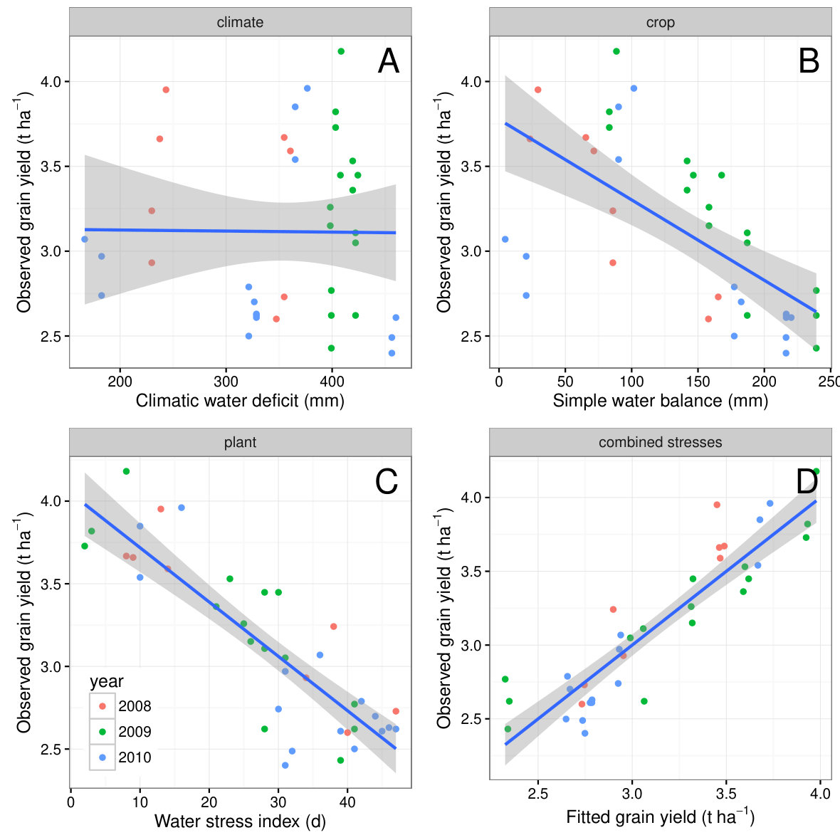 Figure 1
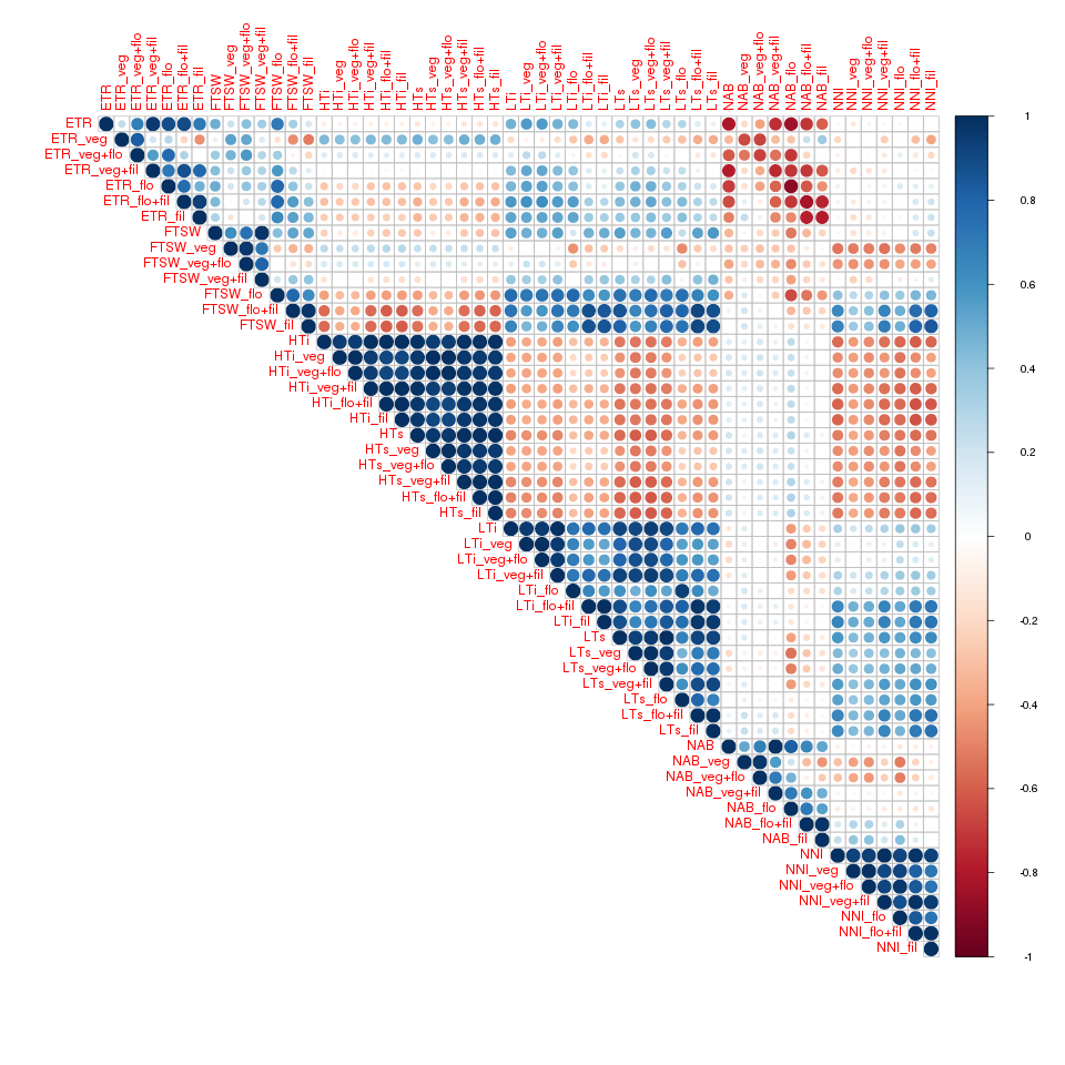 Figure 2
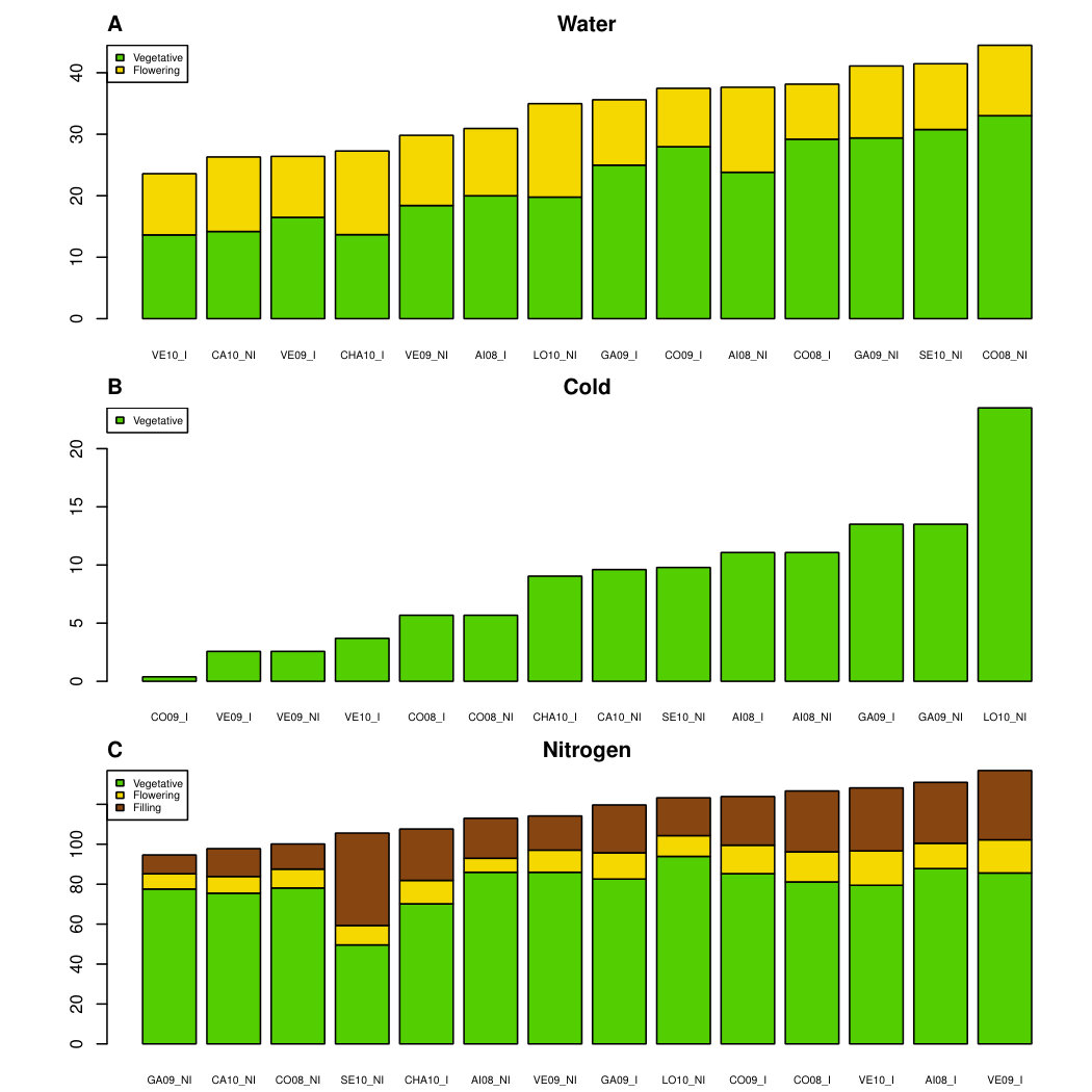 Figure 3
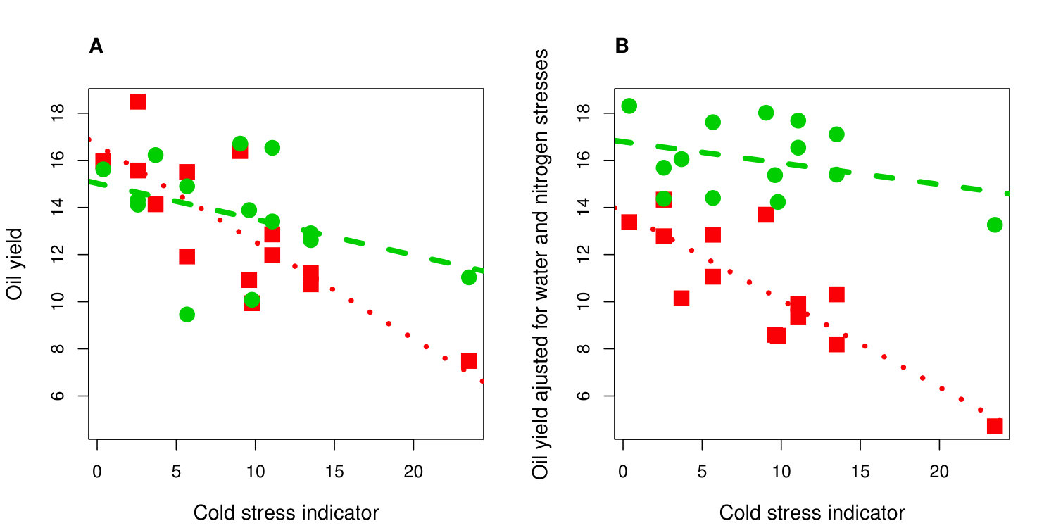 Figure 4
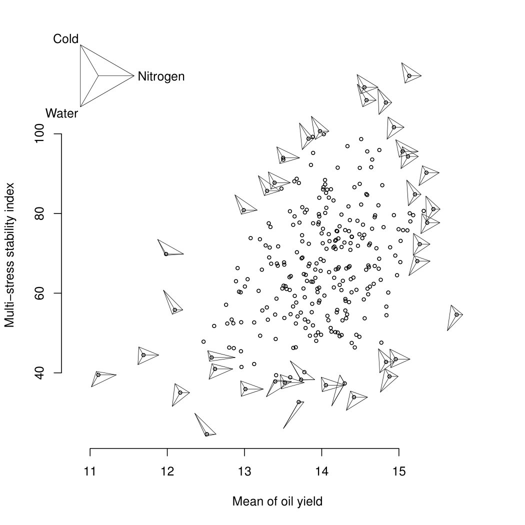 Figure 5
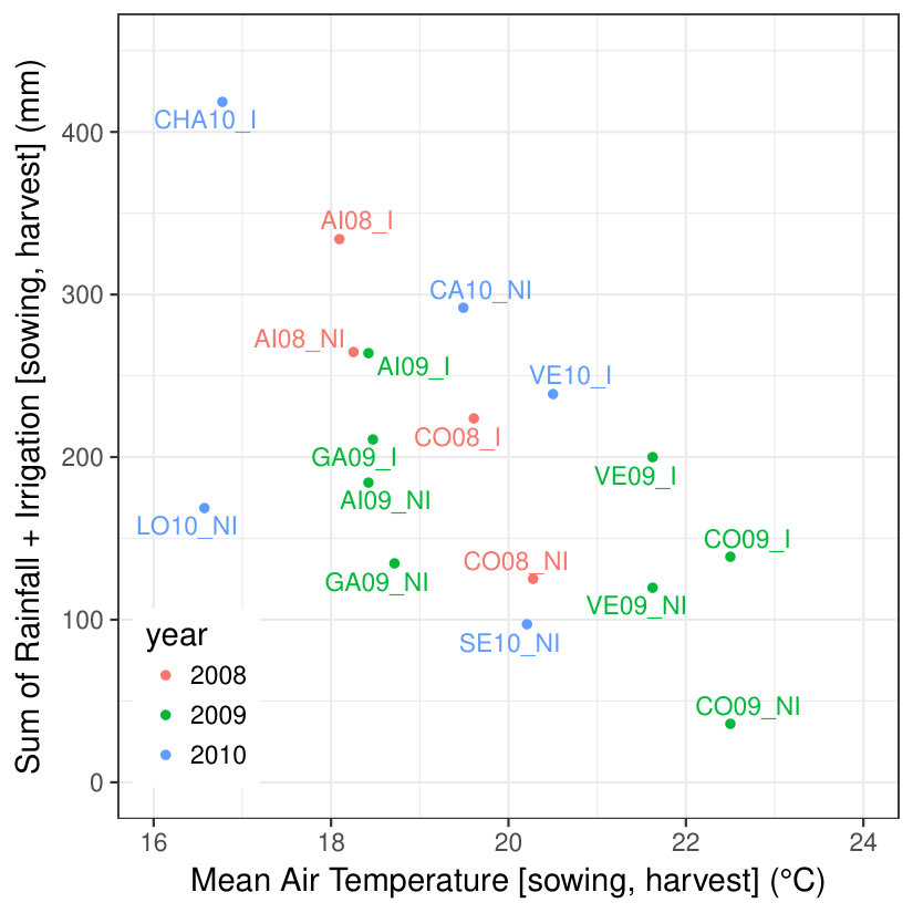 Figure 6
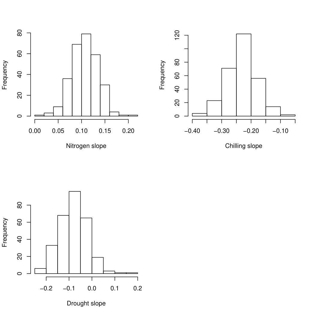 Figure 7
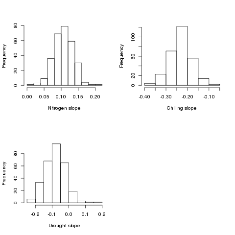 Figure 8
| Environment | Locationa | Treatmentb | Year | Tester for B-line | Tester for R-line | Number of lines |
|---|---|---|---|---|---|---|
| AI08_I | AI | I | 2008 | 83HR4gms | T1 | 192 |
| AI08_NI | AI | NI | 2008 | 83HR4gms | T1 | 193 |
| CO09_I | CO | I | 2009 | 83HR4gms | T1 | 278 |
| CO09_NI | CO | NI | 2009 | 83HR4gms | T1 | 278 |
| GA09_I | GA | I | 2009 | 83HR4gms | T1 | 275 |
| GA09_NI | GA | NI | 2009 | 83HR4gms | T1 | 274 |
| LO10_NI | LO | NI | 2010 | 83HR4gms | T1 | 284 |
| VE10_I | VE | I | 2010 | 83HR4gms | T1 | 289 |
| AI09_I | AI | I | 2009 | T2 | T3 | 280 |
| AI09_NI | AI | NI | 2009 | T2 | T3 | 280 |
| VE09_I | VE | I | 2009 | T2 | T3 | 273 |
| VE09_NI | VE | NI | 2009 | T2 | T3 | 273 |
| CA10_NI | C1 | NI | 2010 | T2 | T3 | 306 |
| CO08_I | CO | I | 2008 | T2 | T3 | 249 |
| CO08_NI | CO | NI | 2008 | T2 | T3 | 249 |
| SE10_NI | SE | NI | 2010 | T2 | T3 | 285 |
| CHA10_I | CHA | NI | 2010 | T2 | T3 | 306 |
| Stress | Symbol | Description | Unit | Formula |
|---|---|---|---|---|
| temperature | HTi | high temperature (continuous) | - | |
| temperature | HTs | high temperature (discrete) | d | |
| temperature | LTi | low temperature (continuous) | - | |
| temperature | LTs | low temperature (discrete) | d | |
| water | FTSW | Edaphic water deficit (continuous) | - | |
| water | ETR | Edaphic water deficit (discrete) | d | |
| nitrogen | NAB | Absorbed nitrogen | kg ha-1 | |
| nitrogen | NNI | Nitrogen deficit (continuous) | - |
| location | year | CWD | AWC | density | sowing | harvest | irrigation |
|---|---|---|---|---|---|---|---|
| AI08_I | 2008 | -239.3 | 144.0 | 6.9 | May-06 | Sep-23 | 70.0 |
| AI08_NI | 2008 | -229.8 | 144.0 | 6.9 | May-06 | Sep-16 | 0.0 |
| AI09_I | 2009 | -408.5 | 240.0 | 6.9 | Apr-24 | Sep-07 | 80.0 |
| AI09_NI | 2009 | -408.5 | 240.0 | 6.9 | Apr-24 | Sep-07 | 0.0 |
| CA10_NI | 2010 | -323.1 | 144.0 | 6.6 | Apr-24 | Sep-11 | 0.0 |
| CHA10_I | 2010 | -177.2 | 112.0 | 6.6 | Apr-30 | Oct-02 | 50.0 |
| CO08_I | 2008 | -356.7 | 190.7 | 6.5 | May-22 | Oct-08 | 98.5 |
| CO08_NI | 2008 | -349.8 | 189.4 | 6.5 | May-22 | Sep-19 | 0.0 |
| CO09_I | 2009 | -421.0 | 174.7 | 6.5 | May-19 | Sep-29 | 103.0 |
| CO09_NI | 2009 | -416.4 | 159.7 | 6.5 | May-19 | Sep-29 | 0.0 |
| GA09_I | 2009 | -422.1 | 160.0 | 6.6 | May-06 | Sep-09 | 75.0 |
| GA09_NI | 2009 | -399.2 | 160.0 | 6.6 | May-06 | Sep-02 | 0.0 |
| LO10_NI | 2010 | -328.5 | 112.0 | 6.9 | Apr-15 | Sep-11 | 0.0 |
| SE10_NI | 2010 | -457.6 | 240.0 | 6.5 | Apr-29 | Sep-30 | 0.0 |
| VE09_I | 2009 | -405.0 | 240.0 | 6.9 | May-07 | Sep-10 | 80.0 |
| VE09_NI | 2009 | -401.4 | 240.0 | 6.9 | May-07 | Sep-10 | 0.0 |
| VE10_I | 2010 | -369.0 | 240.0 | 6.9 | May-07 | Sep-10 | 35.0 |
| Parameter | Unit | Melody | Pacific | Pegasol |
|---|---|---|---|---|
| Temperature sum to floral initiation | °C d | 542 | 531 | 522 |
| Temperature sum from emergence to the beginning of flowering | °C d | 941 | 922 | 906 |
| Temperature sum from emergence to the beginning of grain filling | °C d | 1,188 | 1,169 | 1,153 |
| Temperature sum from emergence to seed physiological maturity | °C d | 1,751 | 1,722 | 1,721 |
| Potential number of leaves at flowering | leaf | 28.7 | 23.5 | 25.3 |
| Potential rank of the plant largest leaf at flowering | leaf | 17.4 | 17.5 | 25.3 |
| Potential area of the plant largest leaf at flowering | cm2 | 537 | 420 | 17.4 |
| Light extinction coefficient during vegetative growth | - | 0.838 | 0.847 | 0.856 |
| Threshold for leaf expansion response to water stress | - | -3.896 | -3.359 | -3.687 |
| Threshold for stomatal conductance response to water stress | - | -10.7 | -10.12 | -9.998 |
| Potential harvest index | - | 0.42 | 0.39 | 0.44 |
| Potential seed oil content | % dry mass | 45.6 | 46.5 | 47.3 |
Peer Reviews
No public reviews on file for this paper yet. If you reviewed it on a platform where reviews are public (OpenReview, ICLR, NeurIPS, ICML), you can paste yours below so the community can read it here.
Videos
No videos yet. Explain this paper in a talk, walkthrough, or lecture? Add one.
Genetic control of plasticity of oil yield for combined abiotic
stresses using a joint approach of crop modeling and genome-wide association
Brigitte Mangin1a, Pierre Casadebaig2a, Eléna Cadic1, Nicolas Blanchet1, Marie-Claude Boniface1, Sébastien Carrère1, Jérôme Gouzy1, Ludovic Legrand1, Baptiste Mayjonade1, Nicolas Pouilly1, Thierry André3, Marie Coque4, Joël Piquemal5, Marion Laporte6, Patrick Vincourt1, Stéphane Muños1, Nicolas B. Langlade1
1 LIPM, Université de Toulouse, INRA, CNRS, Castanet-Tolosan, France
2 AGIR, Université de Toulouse, INRA, INPT, INP-EI PURPAN, Castanet-Tolosan, France
3 Soltis, Domaine de Sandreau, Mondonville F-31700 Blagnac, France
4 BIOGEMMA SAS, Domaine de Sandreau, Mondonville F-31700 Blagnac, France
5 SYNGENTA SEEDS, 12 chemin Hobit, F-31790 Saint Sauveur, France
6 RAGT 2n, Site de Bourran, F-12000 Rodez, France
aThese authors contributed equally to this work
Abstract111This is the
post-print version of the manuscript published in Plant, Cell, and Environment (10.1111/pce.12961)
Understanding the genetic basis of phenotypic plasticity is crucial for predicting and managing climate change effects on wild plants and crops. Here, we combined crop modeling and quantitative genetics to study the genetic control of oil yield plasticity for multiple abiotic stresses in sunflower.
First we developed stress indicators to characterize 14 environments for three abiotic stresses (cold, drought and nitrogen) using the SUNFLO crop model and phenotypic variations of three commercial varieties. The computed plant stress indicators better explain yield variation than descriptors at the climatic or crop levels. In those environments, we observed oil yield of 317 sunflower hybrids and regressed it with three selected stress indicators. The slopes of cold stress norm reaction were used as plasticity phenotypes in the following genome-wide association study.
Among the 65,534 tested SNP, we identified nine QTL controlling oil yield plasticity to cold stress. Associated SNP are localized in genes previously shown to be involved in cold stress responses: oligopeptide transporters, LTP, cystatin, alternative oxidase, or root development. This novel approach opens new perspectives to identify genomic regions involved in genotype-by-environment interaction of a complex traits to multiple stresses in realistic natural or agronomical conditions.
Introduction
Adaptation to climate change requires new crop varieties adapted to new management options. Adaptation of agriculture is a key factor to lessen the impact of climate change (Lobell et al., 2008). The crop exposition to unfavorable growing periods can be partially controlled by adapting crop management, i.e by shifting planting dates or choosing a cultivar with an adequate phenology (Acosta-Gallegos and White, 1995). But such adaptations also have side-effects and while flowering can be successfully desynchronized from the period of occurrence of water deficit, crop emergence would be more exposed to cold stress. In this case, adaptation to climate change should also include the development of new crop varieties (Rosenzweig et al., 1994), with new or improved properties such as tolerance to cold or other abiotic stresses. Moreover, because the multiplicity of cultivation conditions (soils, climatic uncertainty), a single genotype can be exposed to random unfavorable growing conditions within its cultivation area, ultimately impacting the expected crop performance. To ensure a stable performance under uncertain conditions, newly developed genotypes not only need to be tolerant, i.e. adapted to a single type of environment (specialisation) but also plastic, i.e. to be able to adapt in most of growing conditions encountered in the targeted cultivation area (Sambatti and Caylor, 2007).
Phenotypic plasticity is a key process for crop productivity under climate change. One way plants will respond to these changes is through environmentally induced shifts in phenotype (phenotypic plasticity) (Nicotra et al., 2010). While the process of phenotypic plasticity is mostly studied on natural systems, its implications on crop productivity under climate change are interesting for plant breeding (DeWitt and Langerhans, 2004; Sadras et al., 2009). Empirically relationships between plant traits and environmental variables (norms of reaction) are known to vary within species in nature as well as in crop species, are considered heritable traits themselves subject to natural or artificial selection (Sambatti and Caylor, 2007; Via and Lande, 1985). However, crop growth in a fluctuating environment generates complex and dynamic interactions between plant and environment, under the control of cultural practices.
It is necessary to unravel and measure abiotic stress levels before assessing plasticity in plant traits. In these conditions, assessing plasticity in plant traits is limited by our capacity to unravel those interactions and estimate abiotic stress levels at the plant scale. Actually, each growth condition creates a unique combination of those stress levels, with possible identical combinations in different growth conditions. For example, crops growing in continental climates might be exposed to both cold (during emergence) and heat (during flowering) stresses; with high temperatures driving a strong evaporative demand and water deficit, which also limits plant nitrogen uptake from the transpired water stream (Kiani et al., 2016). Accordingly, in a given cultivation area, stresses are not independent (Vile et al., 2012) and need to be characterized and modelled prior studying their impact on plant traits.
Crop simulation and modeling can help to characterize environment from the crop point of view. Because the environment is the largest component of the phenotypic variability of most plant traits and of course crop yield, its quantitative characterization is of major importance (Lake et al., 2016). Crop simulation models are based on mathematical equations representing the crop growth and development as a function of environment (climate, soil and management). Such tools can give access to plant-level state variables, such as time-series of several abiotic stresses, in large range of growing conditions otherwise difficult to characterize with sensors. This methodology was recently implemented and allowed to identify major types of water deficit patterns for rainfed wheat in the Australian target population of environments (Chenu et al., 2013) or for coupled thermal and water stress patterns for chickpea in Australian National Variety Trials (Lake et al., 2016). In sunflower, a crop model was developed by Casadebaig et al. (2011) and takes into account water, cold, heat, and nitrogen stresses to estimate their impact on grain yield and oil content.
Genetic studies of genotype-by-environment interaction (GxE) Although plasticity has long been recognized as an interesting trait in ecological and crop science since the pioneering work of Bradshaw in the 1950s, the identification of genetic variation involved in plasticity is scarce and recent. An approach to deal with phenotypic variation due to environmental effects is to develop multi-environmental QTL analysis to identify QTLxE interactions as reviewed in Van Eeuwijk et al. (2010). Although this approach was widely used for single or multiple traits, this can provide a greater sensitivity for environment-dependent QTL, inform on the stability of the QTL effect, but not on the environmental factor(s) the QTL is responding to. To overcome this issue, several studies compared two conditions, varying a single environmental factor and were able to study the genetic control of the plasticity to a specific stress for a particular trait (El-Soda et al., 2015; McKay et al., 2008). Several genes involved in GxE have been cloned in plants (reviewed by Des Marais et al., 2013) by using a combination of fine QTL mapping and candidate gene approaches. Most genes are involved in flowering time control (FT, PPD1, FLC, FRI, PHYC, CO). Examples concerning abiotic stress responses are still rare: CBF2 for cold stress (Alonso-Blanco et al., 2005), P5CS1 for osmotic stress (Kesari et al., 2012), SUB1A for submersion in rice (Fukao et al., 2011) and RAS1 for saline stress tolerance (Ren et al., 2010). No gene showing a GxE interaction for drought stress nor for any yield-related trait were cloned or fine-mapped yet. This certainly lies respectively in the difficulty to characterize drought stress in natural conditions and in the complex genetic architecture of yield-related traits, which implies small effect mutations. Indeed successful examples were obtained with easy-to-phenotype traits (flowering time) and easy-to-setup environmental factors controlled one at a time.
This reductionist vision of the environment prove to be efficient for gene cloning. However, more complex and realistic approaches are needed to understand plant and crop responses to environmental factors and therefore breed for trait plasticity ultimately providing stable crops. In the context of the phenomics era (Großkinsky et al., 2015), with a greater description of the environment, and with the genomic tools accessible on many species, these approaches should flourish. However, to our knowledge, no study tackled yet the identification of the genetic control of plant plasticity to combined environmental factors in nature or field trials (Mahalingam, 2015). Thanks to prior crop modeling, this approach is now amenable, and shall take advantage of a precise description of the plant stress factors, of the statistical power of multi-environment trials and of the realistic nature of the measured traits.
In this study, we developed a novel approach that combined crop modeling and quantitative genetics to identify the genetic basis of oil yield plasticity in sunflower. Our methodology consisted in estimating four abiotic stress indicators in a range of environments using a crop model and in selecting the indicators explaining the best the grain yield plasticity of commercial varieties. The plant-level stress estimations on these varieties were used to characterize each experimental sites for the three selected abiotic stresses. We could then estimate the plasticity of oil yield for each stress and for every hybrid of a sunflower diversity panel cultivated in every site. Therefore, as a demonstration on cold stress, we could successfully perform a genome-wide association study to identify genomic regions putatively involved in oil yield plasticity to cold.
Material and methods
Plant material
Association mapping was carried out on a panel of 317 inbred lines from INRA and sunflower breeding companies. This panel was a subset of the core collection of 384 inbred lines of Cadic et al. (2013) chosen for its diversity from an initial set of 752 inbred lines (Coque et al., 2008). It was comprised of both elite lines, parents of commercial hybrids, and lines with introgressions from several wild Helianthus accessions, including H. annuus, H. argophyllus and H. petiolaris.
Oil yield was observed on testcross progeny obtained by crossing panel lines with testers according to their status (maintainers of cytoplasmic male sterility [B-lines] or fertility restorers [R-lines]), as described in Cadic et al. (2013). R-lines were crossed with the two CMS PEFS71501 counterparts of B-line proprietary testers (FS71501 or AT0521) while the B-lines were crossed with two R-line testers: 83HR4gms and SOLR001M. 83HR4gms is derived from the 83HR4 line and was converted to female by the introduction of a genetic male sterility, SOLR001M is a proprietary line carrying PEF1 cytoplasmic male sterility (Crouzillat et al., 1991; Serieys, 1984) which it maintains, although it is a restorer for classical PEFS71501 cytoplasm (Table 1).
Description of the multi-environment trial
(MET)
From 2008 to 2010, eight locations located in the center and Southwest of France were planted with the testcross progeny. In six location, trials were conducted with and without irrigation, providing a total of 17 location x treatment x year combinations, (designated as environments). The panel lines were evaluated on the same tester in each environment (Table 1). Each experiment was an Augmented-Design (Federer, 1961) formed of blocks, with 24 or 30 entries replicated in two sub-blocks. Each sub-block was randomized separately and contained two to four control hybrids.
Table 1. Details on location, treatment, year, testers and observed hybrids for the 17 environments.
The climatic variability on experimental locations was summarized by computing the mean air temperature, the sum of water inputs (rainfall and irrigation) and the climatic water deficit (difference between precipitations, P and potential evapotranspiration, PET) on the cropping period (see supplementary Figure S1 and Table S1). No environment had a climatic water deficit (ranging from -177 to -458 mm), meaning that the climatic evaporative demand was always above the water supply (even accounting for irrigation). Rainfall on the cropping period ranged from a low 36 mm to 368.5 mm and the average amount of irrigation was 74 mm. Trials were performed on various soils depth leading to a soil water capacity (SWC) from 112 mm to 240 mm. Mean nitrogen fertilization was 60 kg/ha (eq. mineral nitrogen).
Among the 17 environments, we discarded 3 environments (AI09_I, AI09_NI, CO09_NI). The first two were outliers for the observed yield and the SUNFLO model failed at simulating yield phenotypes close to the observed one for the controls. The last one did not exhibit genotypic effect for the panel phenotypes, the estimated genotypic variance was judged non-significantly different from zero by a Z-ratio test in the naïve linear mixed model used to correct for micro-environment effects and to predict the BLUP genotypic value of the yield panel lines.
Intra environment phenotypic data
analysis
Within each environment, the oil yield was adjusted for micro-environment effects using ASReml-R (Butler et al., 2009), as described in Cadic et al. (2013). A linear mixed model (named naïve in Cadic et al., 2012) with a random effect for the genotypic value of the panel lines, including blocks and sub-blocks as fixed effects was compared to two spatial models. The spatial models included (a) random effects of row and column or (b) a first-order autoregressive process in the residuals to take into account autocorrelation between neighbour plots. The three models were compared using the Akaike criterion (AIC) and the best linear unbiased predictors (BLUP) of the genotypic values were extracted from the best model according to AIC, for the next step of analysis.
Estimation and choice of abiotic stresses in each
environment using simulation
SUNFLO is a process-based model for the sunflower crop which was developed to simulate the grain yield and oil concentration as a function of time, environment (soil and climate), management practice and genetic diversity (Casadebaig et al., 2011; Debaeke et al., 2010; Lecoeur et al., 2011). The model simulates the main soil and plant processes: root growth, soil water and nitrogen content, plant transpiration and nitrogen uptake, leaf expansion and senescence and biomass accumulation, as a function of main environmental constraints (temperature, radiation, water and nitrogen deficit).
This model is based on a conceptual framework initially proposed by Monteith (1977) and now shared by a large family of crop models (Brisson et al., 2003; e.g. Jones et al., 2003; Keating et al., 2003). In this framework, the daily crop dry biomass (DMt) is calculated as an ordinary difference equation (Equation 1) function of incident photosynthetically active radiation (PAR, MJ m-2), light interception efficiency () and radiation use efficiency (RUEt, g MJ-1, Monteith (1994)). The light interception efficiency is based on Beer-Lambert’s law as a function of leaf area index (LAIt) and light extinction coefficient ().
[TABLE]
Broad scale processes of this framework, the dynamics of LAI, photosynthesis (RUE) and biomass allocation to grains were split into finer processes (e.g plant phenologic development, leaf expansion and senescence, response functions to environmental stresses) to reveal genotypic specificity and to allow the emergence of GxE interactions. Globally, the SUNFLO crop model has about 50 equations and 64 parameters (43 plant-related traits and 21 environment-related). When evaluated on the presented MET dataset, the SUNFLO model predicted accurately the performance of control hybrids across environments: the root of mean square error (RMSE) was 0.3 t ha -1, relative RMSE was 9.6 %, bias was -0.14 t ha-1.
Using the SUNFLO model, we computed two indicators (continuous and discrete) per type of considered abiotic stresses to characterize the different environments (Table 2). Each indicator was integrated over three key periods: vegetative stage (veg), flowering period (flo) and grain filling period (fil). We also considered the sum over two periods and during the whole cropping period, for a total of seven time periods per indicator. All these indicators corresponded to the mean stress felt by the control hybrids during the above periods.
For water stress, the fraction of transpirable soil water (FTSW) represents yield limitation through water deficit (integration of 1 minus FTSW); ETR is the conditional sum of days, if the ratio of the real evapotranspiration (ET) to potential evapotranspiration (PET) was less than 0.6 (threshold for photosynthesis limitation). For cold stress, LTs is the conditional sum of days if mean air temperature was below 20°C and LTi represent low temperatures impact on photosynthesis (integration of 1 minus equation 2). Heat stress indicators were computed following the same logic, albeit representing high temperatures impact on photosynthesis. Equations (2) and (3) are used in the crop model to define the radiation use efficiency (RUE) response to temperature (Villalobos et al., 1996). For nitrogen deficit, NAB is the amount of absorbed nitrogen in the considered cropping period and NNI is the sum of 1 minus nitrogen nutrition index, which indicates crop nitrogen deficit (Debaeke et al., 2012; Lemaire and Meynard, 1997).
[TABLE]
[TABLE]
where denotes the mean daily air temperature (°C), is the base temperature (°C), is the optimal lower temperature (°C), is the optimal upper temperature (°C) and is the critical temperature (°C).
Table 2. Description of abiotic stress indicators simulated by the crop model.
Three sunflower varieties (Melody, Pacific, Pegasol) which were used as controls within the environments had their phenotypic characteristics previously included in the SUNFLO model (Supplementary Table S2). The soil characteristics, the crop management and climate data were collected to allow simulation for each environment. One soil characteristic, the soil depth, is difficult to observe and has a strong impact on the simulated yield. Instead of using the approximated value given by the breeders and the farmers, we adjusted this parameter by minimizing the empirical mean square error between the observed and the simulated yields.
Model choice to select the stress indicators was made with the AIC using the native R function lm. AIC of each model was computed for all three control varieties and model choice was made on the mean over the three controls. Compared linear models, which fitted the grain yield with the indicators, were limited to combinations of only one indicator per type of stresses. All models integrating one, two, three or four stresses were compared; in total 50,624 models were computed and compared.
The R function lm was also used to compute the p-value of the Fisher test for each indicator including in the best model.
Genetic study
Estimation of plasticities of oil yield to water, nitrogen
and cold stresses in the diversity panel
In order to get plasticity phenotypes that reflect the responses of the panel lines to the different abiotic factors, we adjusted the BLUP phenotype of each panel line with the following linear model:
[TABLE]
where is the BLUP of the phenotype for the th genotype, the potential phenotype in an environment with average stresses, the water stress indicator in the th environment calculated as the mean over the 3 controls, the slope linked to the water stress, the cold stress indicator in the th environment calculated as the mean over the 3 controls, the slope linked to the cold stress, the nitrogen stress indicator in the th environment calculated as the mean over the 3 controls, the slope linked to the nitrogen stress and the residual variance. The covariates , , and were centered before computing the regression model. The three estimated covariate coefficients , , and of this model are the plasticity phenotypes of interest, i.e. the genotype slopes in response to water, cold and nitrogen stresses respectively. To compare model (4) to a more simple regression model, we also fitted the BLUP phenotype of each panel line using the cold stress indicator as a single regressor.
Before computing the above linear model, the oil yield missing data were imputed using the missMDA R package (Josse et al., 2012; Josse and Husson, 2016). All recorded traits (24 traits for a total of 198 traits x environments) were used to impute missing oil yield values. However, panel lines with less than six observations per oil yield trait over the environments were discarded.
Combined stresses in a single multi-stress index of
plasticity
In order to compare the panel lines for the stability against multiple stresses together, we defined a multi-stress plasticity index accounting for the variance-covariance of the stress slopes, equals to:
[TABLE]
where denotes the (3 by 3) variance-covariance matrix.
To visualize the strategy of the panel lines versus the three stresses, we drew a star representation using the star function of the R package graphics. The three plasticity phenotypes were first taken in absolute value and scaled to 0-1 in order to have three comparable values with values close to 0 noted the stability and values close to 1 noted the instability. Then they were normalized by panel line to sum to 1 in order to get comparable values for all panel lines. The star representation was applied on these scaled and normalized values that can be interpreted as the percentage of stability dedicated to each stress.
Genotyping and map
building.
A set of 197,914 SNP were used to produce an AXIOM® genotyping 96-array (Affymetrix, Santa Clara, CA, USA). These SNP were selected from either genomic re-sequencing or transcriptomic experiments. An additional set of 6,800 non-polymorphic sequences were added as controls. Combined with internal technical controls, the AXIOM® genotyping 96-array was designed with a total of 445,876 probesets.
Genomic DNA from the 317 panel lines and two recombinant inbred lines (RIL) populations INEDI and FUxPAZ2 obtained from the cross between XRQ and PSC8 lines (180 RIL) and from the cross between FU and PAZ2 lines (87 RIL) respectively, were genotyped with the AXIOM® array. All hybridization experiments were performed by Affymetrix and the genotypic data were obtained with the GTC software (Affymetrix). From the 197,914 SNP, 35,562 were polymorphic between XRQ and PSC8 and 28,529 between FU and PAZ2.
We used CarthaGène v1.3 (Givry et al., 2005) to build the genetic maps of the INEDI population and the FUxPAZ2 population separately. For the INEDI population, we added to the set of AXIOM® SNP the markers previously mapped by Cadic et al. (2013) which allowed completing this map and assigning AXIOM® markers to appropriate linkage group (LG). We built a consensus map with common markers of both previous maps using Biomercator v4.0 (Sosnowski et al., 2012) and we projected the specific markers of the two previous maps on this consensus map. Unmapped AXIOM® SNP were placed by BLAST analysis on the RHA280xRHA801 genetic map based on 454 sequencing (Kane et al., 2011) and finally projected on the INEDI and FUxPAZ2 consensus map. The remaining AXIOM® SNP were located by computing the linkage disequilibrium (LD) measurements proposed by Mangin et al. (2012). They were mapped to the same position of the mapped SNP in maximum LD. For this, we used as LD statistics the maximum of the and measurements that correct for relatedness and for both structure and relatedness, respectively.
Association tests
Association mapping was based on a set of 65,534 SNP with MAF
0.05. Similarly to our previous work (Cadic et al., 2013), two association models were performed using EMMA (Kang et al.,
- based on the Yu et al. (2006) model. Both models included a correction for the genomic relatedness using the alike-in-state (AIS) kinship estimated with EMMA version v1.1.2 R package (Villanova et al.,
- using all the above SNP. The population structure modelled as the restorer or maintainer status of the panel lines was added in the second model leading to the following model:
[TABLE]
is the slope for ith line, is the line status, is the effect of the line status , is the genotype of the ith line at locus l, is the effect of locus l. and are considered to be fixed effects. is the random polygenic effect modeling genetic relatedness with where is an AIS matrix and where denotes the identity matrix. Multiple testing correction was achieved using an approximate effective number of tests () based on the eigen-values of the SNP correlation matrix as proposed by Li and Ji (2005). We computed by using blocks of 250 markers and assuming that the blocks were independent.
In order to conduct a multi-loci analysis, the genotypic data was imputed using Beagle v4.0 (Browning and Browning, 2007) and MLMM (Segura et al., 2012) was used for this purpose. We stopped the forward approach of MLMM when the variance of the polygenic term was non significant, which is a little different compared to the initial forward procedure of MLMM that stops when the estimator of this polygenic variance is equal to 0. The significance of the polygenic variance component was judged with a log-likelihood ratio test and a risk of 1%. This log-likelihood ratio test compared the model with and without the polygenic effect. Two times the difference between the log-likelihood of the models is known to follow asymptotically a mixture between a Dirac at 0 and a Chi-square distribution with 1 degree of freedom (Self and Liang, 1987). When the forward approach stopped, a SNP was judged associated if its Bonferonni corrected p-value, using as the number of independent tests, was inferior to the chosen type I error. The associated SNP were put all together with the polygenic term to create the final multi-loci linear model. The associated SNP effect, their reevaluated p-values were computed with the base R function lm in this final model (R Core Team, 2014).
Functional annotation of associated
SNP
Context sequences of associated SNP were compared to the sunflower genome (line XRQ) sequenced using the PacBio (Pacific Biosciences, Menlo Park, CA, USA) technology (https://www.heliagene.org/HanXRQ-SUNRISE/) by blast analysis. In case of ambiguous positioning on the genome, we retained the chromosomal position in accordance to genetic map location of the marker. Similarly, we positioned associated SNP on the reference transcriptome (https://www.heliagene.org/HaT13l/) All SNP were situated in gene coding regions, the sunflower genes, the best Arabidopsis hit with its description in TAIR10 are indicated in Table 5.
Results
Estimation of abiotic stresses in field
environment.
The characterization of abiotic stresses at the plant level through modeling and simulation explained observed yield varibility better than climate-based indicators (Figure 1). For example, the correlation between yield observed in field experiments and water deficit computed from (1) climate data only (P - PET), (2) climate, soil, and management data (P - PET + SWC + irrigation) and (3) simulated plant data (ETR, defined in Table 2) was gradually stronger (respectively -0.01, -0.65 and -0.86). The correlation between yield and water deficit index increased in strength with the “proximity” of the regressor to the plant, revealing the expected negative impact of water deficit on crop yield.
Figure 1. Relation between observed grain yield and several abiotic stress indicators
The correlation between different type of abiotic stresses (Figure S2), indicated that cold (LT) and heat stresses (HT) were naturally the most highly negatively correlated combination. The nitrogen indicator NAB was not correlated to other indicators except the negative correlation with the water stress indicator (ETR, particularly during grain filling). The other nitrogen indicator NNI, which was not correlated to NAB showed both a positive correlation with heat stress indicators and a negative correlation with cold indicators. The water stress indicator FTSW during grain filling was also positively correlated to heat stress indicators (HT), nitrogen stress (NNI), and negatively correlated to cold stress indicators. Within a single type of stress, correlations between indicators computed during different cropping periods were generally positive and high (Figure S2), ranging 0.40 for water deficit (FTSW) to 0.98 for heat stress (HTi), with nitrogen and cold indicators in-between.
Figure 2. Heat map of the correlations between stress indicators.
Model selection to estimate the best combination of
abiotic stresses.
The model selected as having the best AIC on average over the control genotypes was a three indicator model, including a cold stress indicator during the vegetative stage (LTi), a water stress indicator during the vegetative and the flowering period (FTSW), and a nitrogen indicator during the whole growth period (NAB). Table 3 presents the p-value of the Fisher test for each control in this best model and the proportion of variance explained by this best model for each control.
Table 3. Results of the regression between grain yield and abiotic environmental indicators: water, cold and nitrogen stresses.
Each stress indicator had a significant effect on the grain yield for each control genotype. The highest impact was due to cold stress for Melody (p-value = 2.39 10-4) and the smallest was due to water stress for Pacific (p-value = 2.91 10-2) as indicated in Table 3. All together these indicators explained very well the grain yield variability of each control since the percentages of explained variance were 90%, 93% and 94% for Pegasol, Pacific and Melody respectively.
Although cold stress has a strong impact on yield (-0.35 q h-1 d-1), the relatively low number of day of cold stress in the MET (8.7 on average, variation in the MET shown on Figure 3) reduces its impact, whereas water stress impacts the most yield due to the high number of days of stress (33.9 on average) even if sunflower is relatively tolerant (-0.14 q h-1 d-1).
Figure 3. Ranges of variation of abiotic stresses in the multi-environment trial.
Plasticity in the diversity
panel.
As we described the actual cold, nitrogen and water stresses felt by sunflower in 14 environments, we also measured oil yield in a diversity panel in those environments. This allowed us to compute plasticities of oil yield to abiotic stresses for each line in the panel as the slopes of regression of oil yield to individual stress indicators. These three slopes represented how plastic was the response of a line faced to a given stress and are therefore referred as plasticity phenotypes later. Minimum, mean, maximum, and variance of these plasticities as well as their correlation are presented in Table 4 and their distribution histograms are in supplementary Figure S2. Cold stress plasticity appears genetically independent to water and nitrogen stress plasticities. On the contrary, nitrogen and water stress plasticity are highly correlated (Pearson correlation of 0.62) suggesting common genetic control of these traits in our panel.
Table 4. Variation and correlation of the plasticities of oil yield for different abiotic stresses in the diversity panel.
To illustrate the importance of multi-stress indicator modelling, we compared regression of oil yield in a single stress indicator model (including only cold stress indicator) and in the multi-stress indicator model in Figure 4. Oil yields of the most sensitive and tolerant lines were plotted against the cold stress indicator. Point clouds are closer to the regression lines in the multi-stress indicator model indicating a better characterization of cold stress impact in this modelling approach.
Figure 4. Regression of oil yield against the cold stress indicator for the most tolerant (green triangles) and sensitive (red squares) panel lines showing the ability of multi-stress modelling to better characterize the environment.
A multi-stress plasticity
index.
Following the estimation of the three single stress plasticities, we were interested in calculating a multi-stress plasticity index to describe the general abiotic tolerance of every line. This index is a weighted sum of the three abiotic stress plasticities taking into account the correlation between them, specifically the one between drought and nitrogen. This index allowed allowed us to rank the panel lines and to describe the different strategies observed in the panel to tolerate combined stresses. This is illustrated on Figure 5 that shows the multi-stress plasticity index of every panel lines against its mean oil yield in the MET. Stable panel lines, with a small multi-stress plasticity index, as well as panel lines belonging to the border of the point cloud were highlighted by a star representation (a triangle in our case) illustrating their abiotic stress tolerance strategy. First, we observed that unstable panel lines were generally more sensitive to cold stress compared to stable lines. This was confirmed by a significant correlation between the multi-stress plasticity index and the percentage of plasticity due to the cold stress (p-value of 6 10-4) although this was not observed for nitrogen or water stress (p-value of 0.28 and 0.10 respectively). Second, we could not identify a consensus strategy for stable panel lines. As examples: (i) the three similarly stable panel lines (multi-stress index around 45) having high oil yield (around 15) developed tolerance to all stresses but showed different plasticity patterns, (ii) the two most stable panel lines had opposite profile of stability with the most stable being sensitive to cold and the second to water.
Figure 5 Relation between the multi-stress plasticity index and the average oil yield showing differences in stress tolerance strategies in the diversity panel of sunflower lines.
Genetic map.
In order to position the genomic regions controlling the abiotic stress plasticity, we constructed a genetic map with the markers genotyped on the diversity panel using three RIL populations. The final genetic map was composed of 89,979 markers positioned in 4,782 genetic positions for a total distance of 1,398.5 cM. On this map, 4,094 markers were used to build the consensus map between the INEDI (XRQxPSC8) and FUxPAZ2 RIL populations. Among the other markers, 27,663 were mapped using the INEDI population alone, 13,807 were mapped using the FUxPAZ2 population alone, 29,586 were located thanks to a genotyping by sequencing map on the RIL population RHA801xRHA280 (Kane et al., 2011) and the remaining 14,829 markers were placed by linkage disequilibrium. Details of these maps can be found in the supplementary Table S3.
Association study of oil yield plasticity to cold
stress.
For the genetic analysis, we focused, as a proof of principle of the approach, on the plasticity to cold stress as it is the most impacting stress and appeared genetically independent from the others. Among the 65,534 association tests, the effective number of tests (Li and Ji, 2005) was estimated around 14,000. Using this effective number of tests, we kept SNP associated with a Bonferroni corrected p-value of 7.1 10-6 for a family wise type I error of 10%. Only 2 SNP were detected by a marker by marker association analysis using EMMA. The most significant SNP was located at the end of LG 5 in a QTL named LG05.64, and was detected with a model including the maintainer or restorer status as a fixed structure effect. The second is located at the center of LG 17 and was detected without the line status effect.
We completed this study by a forward approach of the multi-loci association analysis (MLMM) for both models (with or without the maintainer/restorer status). Both models stopped with 6 SNP among which four were judged associated. None of them was common between both models but one SNP corresponded to the previously found SNP in LG05.64. The most associated SNP was located at the end of the LG13. In total 9 QTL could be identified: two located on chromosomes 5 and 10 and one on chromosomes 9, 13, 14, 16 and 17. Their phenotypic effects on cold stress plasticity varies from 10 to 21% of the average plasticity in the panel (Table 5).
Table 5. Positions and estimated effects of SNP and genes associated with oil yield plasticity to cold stress.
Genes located in QTL controlling oil yield plasticity to
cold stress.
We were interested in genes containing associated SNP to link the genetic identification to molecular and physiological processes putatively involved in cold tolerance. All associated SNP were located within coding sequences as expected from the AXIOM® genotyping array design. Functional annotation of the corresponding genes pointed out homologues of: NPF3.1, LTP, CYS6, NPF5.3, GMII, RPD1, PPX1, HAOX2 and IAR4 (from the most to the least significantly associated, as shown in Table 5). Strikingly, two close homologues of oligopeptide transporters (NPF3.1 and NPF5.3) are present in associated QTL on LG 5 and 14 and two homologues of genes involved in root development (RPD1 and IAR4) on LG 9 and 17. In addition, homologues of a lipid transfer protein, a cystatin, an alpha-mannosidase, a protein phosphatase and an aldolase are also in QTL controlling oil yield plasticity to cold stress.
Discussion
In this work, we developed a novel method to characterize the abiotic stress levels on different environments by using crop modeling and simulation and subsequently exploited it to identify genetic control of stress plasticity. We implemented this environment characterisation method on 17 locations from a multi-environment trial for sunflower and four abiotic stresses (water, nitrogen, cold and heat). The SUNFLO model (Casadebaig et al., 2011) was used to simulate stress patterns dynamics for three varieties used as controls in each location and integrated indicators were computed from these data considering different crop phenological stages and physiological processes (eight stress indicators over seven periods). We used a model selection approach to select the best linear model among combinations of stress indicators used as regressors for yield. Water, nitrogen and cold stresses were retained as the most explicative abiotic stresses for yield variability in this MET. Using reaction norms as conceptual reference, we computed abiotic stress plasticities as the slopes of the linear regression of oil yield on selected stress indicators. We then conducted an association study with a panel of 317 lines genotyped for nearly 65,000 markers on oil yield plasticity for cold stress as its was the most impacting stress (per time unit) and was not correlated to other abiotic stress plasticities.
Crop modelling helped to analyze abiotic stress patterns
and to explain their impact on yield.
In a location, stress indicators can be climate-based (precipitations minus evapotranspiration), crop-based (simple water balance including soil water capacity and irrigation) or plant-based (simulated dynamic water balance). We observed that the observed grain yield was best explained by plant-based stress indicators because the interactions between climate, leaf area dynamics, plant stomatal conductance (isohydric vs anisohydric behaviours, e.g. Casadebaig et al. (2008) for sunflower) and management practices can be partly reproduced by the crop model algorithm. This is for example illustrated by environment rankings, where some irrigated locations (CO08_I, CO09_I) can still display a high level of water stress while a rainfed one (CA10_NI, VE09_NI) show reduced water deficit.
Abiotic stresses also do not have the same impact on crop physiology according to their timing of occurrence during the crop cycle (Table 3). Among the seven possible combinations between main crop phases (i.e. vegetative, flowering, grain filling), we indeed observed that the relevance of these timings was specific to the type of abiotic stress. For cold stress, the detection of early crop growth (vegetative period) was expected because this stress occurrence is strongly determined by the climate (low temperature during crop installation). However, in continental climates, where sunflower is mainly grown, we can also observe cold temperatures at the end of the crop cycle. For water stress, where interactions between crop growth and climate variability are more important, vegetative and flowering periods were identified, which is consistent with numerous previous reports on sunflower (Blanchet et al., 1990; Cabelguenne et al., 1999). Regarding nitrogen stress, the importance of this process over the whole crop cycle was highlighted. Indeed, recent reports indicated that post-flowering nitrogen absorption could also be significant (Andrianasolo et al., 2016). Remarkably, heat stress was not identified as a major contribution to yield variability in the MET. Actually, depreciative effect of high temperatures on photosynthesis were caused by temperatures that were almost never reached in our experimental conditions. According to the current parameterization of the simulation model, heat stress indicator (3) was only significant in one location (CO09) and null (9/17 locations) or weak in the others (Figures 2 and S1).
Genetic control of plasticity of oil yield to cold
stress
The most and fourth most associated SNP pointed to two genes highly homologous to NPF3.1 and NPF5.3 that are both oligopeptide transporters. These two independent association signals on chromosomes 5 and 14 strongly suggest a role of oligopeptide transport in tolerance to cold stress observed in our experimental conditions i.e. when young plants are exposed to chilling. In plants, these transporters are key players in nitrogen nutrition and therefore plantlet growth. The importance of oligopeptide transport to tolerate cold is corroborated by the demonstrated molecular adaptation of this transporter family in antarctic icefish (Chionodraco hamatus) adapted to sub-zero temperatures (Maffia et al., 2003; Rizzello et al., 2013). The role in N nutrition of these transporters in animal and plants indicates that nutrient transport can be a limiting factor at low temperature that likely limits remobilization of seed stocks and/or absorption and transport of N from roots to aerial organs.
The second most associated SNP is located in a putative lipid transfer protein (LTP) (QTL LG16.48). Many LTP have been reported to be transcriptionally induced by freezing (reviewed in Liu et al., 2015) and over-expression of LTP3 provided freezing tolerance in A. thaliana (Guo et al., 2013). This action could be due to membrane stabilization as demonstrated by Hincha et al. (2001) in preventing chloroplastic damages induced by freezing, or through its role in seed lipid mobilization during germination and seedling growth (Pagnussat et al., 2015) as shown in sunflower for another LTP (Pagnussat et al., 2009). Another candidate genes is the cystatin CYS6 homologue located in QTL LG13.72. Several homologues of cystatin were shown to be induced during cold exposure in barley (Gaddour et al., 2001), maize (Massonneau et al., 2005), wheat (Talanova et al., 2012), and increase, when over-expressed, cold tolerance in Arabidopsis (Zhang et al., 2008). Based on Prins et al. (2008), the sunflower cystatin could provide a better regulation of Rubisco turnover in chloroplasts in cold conditions. The alternative oxidase HAOX2 homologue found in QTL LG10.34 constitutes another good candidate gene for cold tolerance. The Alternative Oxidase Pathway (AOP) has been described in many plants to be involved in cold stress response as a biochemical protection against overproduction of Reactive Oxygen Species due to the cold inhibition of the electron transport chain in mitochondria (Feng et al., 2008). Furthermore, the AOP was shown to participate in differential cold-sensitivity between two maize genotypes (Ribas-Carbo et al., 2000).
Interestingly, Interestingly, two genes (homologues to RPD1, IAR4) were found (QTL LG09.27, LG17.49) and their Arabidopsis counterparts share similar features: both are involved in root development and both mutants show temperature-sensitive phenotypes (at 20°C and 28°C) (Konishi and Sugiyama, 2006; Quint et al., 2009). This suggests that root setting could also be temperature- and genotype-dependent in sunflower. All together, the functional annotation of QTL associated to cold stress plasticity of oil yield identified several candidate genes and physiological processes. Most of them were already described to be involved in cold stress tolerance in other plants which supports our study and indicates a probably short genetic distance between associated SNP and causal mutations.
To complete our understanding of how these processes that act during the early growth phase of sunflower, impact the final seed yield, further studies putting in relation dynamic measurements of plant growth rate and cell physiology would be enlightening.
Phenotypic plasticity and tradeoff for potential
yield
In the studied multi-environment network, mean oil yield was positively correlated with a high sensitivity to environmental stresses, indicating that a global gain in performance was generally associated to a higher yield instability (Figure 5). This is globally in accordance with previous claims that an increase in phenotypic plasticity allowed to achieve better yield stability across environments but at the expense of greater performance in low stress conditions (Sadras et al., 2009). However the presence of both high-yielding and stress-tolerant genotypes suggests this general observation can be genetically by-passed and leaves room for more efficient sunflower varieties.
Stability of complex traits such as yield or fitness depends on plasticity of numerous intermediate traits (likely physiological and developmental processes) that are yet unknown. In our approach, we studied directly the plasticity of the complex trait with the idea of stabilizing it. The molecular and physiological processes pointed out by the genetic analysis allow us to identify some candidate processes: oligopeptide transport, root development, ROS scavenging, chloroplast and mitochondrial physiology (i.e. intermediate traits). In this kind of approach, we can wonder whether we could detect key regulators such as transcription factors (none in our case). Indeed, genetic variation in those would likely have trade-off effects on various physiological processes. Then, they would impact intermediate traits significantly but with possibly opposite effects and at the end, no significant impact on the resulting complex trait.
On the breeding strategy point of view, the considered environmental stresses (temperature, nitrogen and water) do not necessarily coexist in the French target population of environments: e.g. south-western production regions are exposed to drought and heat stress while the temperatures in northern regions are low enough and necessitate short crop cycle cultivars. This lack of spatial superposition of environmental constraints allow to exploit the differential sensitivities in the studied genetic material and adapt cultivar choice or breeding according to local growing environment. On the other hand, breeding for phenotypic plasticity of intermediate traits would potentially result in resilience to increasingly unpredictable environments (Nicotra et al., 2010).
Conclusions
Improving crop performance in low-input cropping systems requires a coordinated improvement of genotypes and agronomical practices (Sadras and Denison, 2016). In these growth-limiting conditions, abiotic stresses occur in combined and dynamic patterns. Therefore, disentangling those using models allows to understand their specific impacts on complex traits (such as yield) and the genetic factors potentially reducing those.
In our study, precise characterization of water, cold, heat and nitrogen stresses allowed accurate identification of nine QTL and underlying genes controlling stress plasticity. This joint approach between crop modeling and quantitative genetics also permitted estimations of allelic variation in natural conditions.
Such inter-disciplinary approach should be useful to conduct different breeding strategies and adapt crop to climate variability through local adaptation: maximizing performance in a given environment type, or through global adaptation: maximizing yield stability over different environment types.
Acknowledgment
This work benefited from the GENOPLANTE program HP1 (2001–2004), the SUNYFUEL project, financially supported by the French National Research Agency (ANR-07-GPLA-0022, 2008–2011), the OLEOSOL project (2009–2012) with the financial support from the Midi Pyrénées Region, the European Fund for Regional Development (EFRD), and the French Fund for Competitiveness Clusters (FUI), and the SUNRISE project of the French National Research Agency (ANR-11-BTBR-0005, 2012-2019).
Table 1 Details on location, treatment, year, testers and observed hybrids for the 17 environments. a The locations were designated as follows: AI: Aigrefeuille (Center West), CA: Castelnaudary (South West), CO : Cornebarrieu (South West), GA: Gaillac (South West), VE: Verdun (South West), LO: Loudun (Center West), SE: Segoufielle (South West), CHA: Chateauroux (Center). b I for irrigation, NI for non irrigation
Table 2: Description of abiotic stress indicators simulated by the crop model. The SUNFLO crop model was used to simulate the interactions between plant growth and available environmental resources. The evolution of resources level and abiotic constraints during the crop cycle was summarized by computing 8 stress indicators during 7 cropping periods: vegetative, flowering, grain filling phase and their combination. equals 1 if is true and 0 else.
Table 3. Results of the regression between grain yield and abiotic environmental indicators: cold, nitrogen and water stresses. Plasticities of the three control genotypes (i.e. commercial varieties) are presented as their slopes and p-values of the type III Fisher test in the best model with the proportion of explained variance for each control genotype. a LTi_veg: integration of low temperatures during the vegetative stage, b NAB: absorbed nitrogen during the whole growth period c FTSW_veg+flo: fraction of the transpirable soil water during the vegetative and the flowering periods. The best explanatory linear model was found by AIC criterion among all the regression models having one to four linear regressors and at most one indicator per stress.
[TABLE]
Table 4. Variation and correlation of the plasticities of oil yield for different abiotic stresses in the diversity panel. Minimum, mean, maximum, and variance of the plasticity phenotypes and their correlations. The plasticity phenotypes are calculated as the slopes in a linear model including the three stress indicators that best characterized the environments. a cold stress plasticity (q h-1 d-1), b nitrogen stress plasticity (q h-1 kg-1), c water stress plasticity (q h-1 d-1)
[TABLE]
Table 5: Positions and estimated effects of SNP and genes associated with oil yield plasticity to cold stress. Genetic distance determined on a consensus map built from three RIL populations (see details in Materials and Methods). Physical position was determined via BLASTing against the genome of line XRQ (early access to version HanXRQv1.1). Association tests were performed using the MLMM procedure unless otherwise stated and either with or without the maintainer/restorer status structure (noted as B/R status). Effects of SNP were estimated using a linear model including all associated SNP. Their relative effect compared with the average plasticity of the diversity panel is indicated. Sunflower gene names correspond to the genome HannXRQ v1.1 (early access). The closest Arabidopsis thaliana homologue is indicated with its TAIR code, name, and a brief functional description.
[TABLE]
(Table continued…)
[TABLE]
Figure 1. Relation between observed grain yield and several abiotic stress indicators. Panels A, B, and C display the regression line between grain yield and water stress indicators, computed at different levels: using climatic data only (panel A, precipitation - potential evapotranspiration, Pearson correlation () of -0.01), using both climatic and crop data (panel B, precipitation - potential evapotranspiration + irrigation + soil water capacity, ) = -0.65, p-value = 9.6 10-6) and using simulated plant data (panel C, evapotranspiration ratio, = -0.86, p-value = 3.3 10-12). Panel D displays grain yield predicted as a function of combined abiotic stresses (linear model of water, nitrogen, and cold stress indicators, = 0.91, root mean square error of 0.21 t ha-1).
Figure 2. Heat map of the correlations between stress indicators. The three selected stress indicators are indicated in blue, yellow and green for water, cold and nitrogen respectively. For water stress, the fraction of transpirable soil water (FTSW) represent yield limitation through water deficit (integration of 1 minus FTSW); ETR is the conditional sum of days, if the ratio of the real evapotranspiration (ET) to potential evapotranspiration (PET) was less than 0.6 (threshold for photosynthesis limitation). For cold stress, LTs is the conditional sum of days if mean air temperature was below 20°C and LTi represent low temperatures impact on photosynthesis (integration of 1 minus equation 2). Heat stress indicators were computed following the same logic, albeit representing high temperatures impact on photosynthesis. Equations (2) and (3) are used in the crop model to define the radiation use efficiency (RUE) response to temperature (Villalobos et al., 1996). For nitrogen deficit, NAB is the amount of absorbed nitrogen in the considered cropping period and NNI is the sum of 1 minus nitrogen nutrition index, which indicates crop nitrogen deficit (Debaeke et al., 2012; Lemaire and Meynard, 1997).
Figure 3. Range of variation in abiotic stresses in the multi-environment trial. Water (A), cold (B), and nitrogen stress (C) indicators, computed by the SUNFLO crop model for each environment, and averaged over the three control genotypes. The SUNFLO crop model was used to compute stress indicators for three control commercial hybrids (Melody, Pacific, Pegasol) according to the developmental stage of the crop: vegetative growth (green), flowering (yellow), and seed filling (brown).
Figure 4. Regression of oil yield against the cold stress indicator for the most tolerant (green triangles) and sensitive (red squares) panel lines showing the ability of multi-stress modelling to better characterize the environment. A) Regression in a single (cold) stress indicator model. B) Regression in a multi-stress (cold, nitrogen, water) indicator model.
Figure 5. Relation between the multi-stress plasticity index and the average oil yield showing differences in stress tolerance strategies in the diversity panel of sunflower lines. The three-branch star represents the strategy of the most extreme panel lines in response to combined abiotic stresses. The length of star branches represents the relative plasticity against the corresponding stress: longer equals more sensitive.
Supplementary data
Table S1. Description of locations and management practices on the multi-environment trial. Headers indicates the locations and years of trials, the climatic water deficit (CWD, mm) i.e.~the sum of precipitation minus sum of potential evapotranspiration, the plant available water capacity (AWC, mm) i.e., the amount of soil water reserves, plant density at sowing (plants m-2), sowing and harvest dates, and the amount of irrigation (mm).
Table S2. SUNFLO genotype-dependent parameters for the three controls.
[TABLE]
Table S3. Marker number, genetic positions (pos.) and genetic distance (cM) of the genetic maps and number of markers positionned by linkage disequilibrium (LD).
Figure S1: Description of the climatic conditions experienced on the multi-environment trial Climatic variability on the experimental network was represented with water (sum of rainfall and precipitations) and temperature (mean air temperature) indices computed on the cropping period (sowing-harvest). The 17 locations x year x management combinations are represented in this space, locations codes are detailed in table S1.
Figure S2. Histograms of the plasticity phenotypes for nitrogen cold and water stresses in the sunflower core collection.
References
Acosta-Gallegos, J., White, J.W., 1995. Phenological plasticity as an adaptation by common bean to rainfed environments. Crop Science 35, 199–204. doi:10.2135/cropsci1995.0011183x003500010037x
Alonso-Blanco, C., Gomez-Mena, C., Llorente, F., Koornneef, M., Salinas, J., Martínez-Zapater, J.M., 2005. Genetic and molecular analyses of natural variation indicate CBF2 as a candidate gene for underlying a freezing tolerance quantitative trait locus in arabidopsis. Plant Physiol. 139, 1304–1312. doi:10.1104/pp.105.068510
Andrianasolo, F.N., Champolivier, L., Debaeke, P., Maury, P., 2016. Source and sink indicators for determining nitrogen, plant density and genotype effects on oil and protein contents in sunflower achenes. Field Crops Research. doi:10.1016/j.fcr.2016.04.010
Blanchet, R., Texier, V., Gelfi, N., Viguier, P., 1990. Articulation des divers processus d’adaptation à la sécheresse et comportements globaux du tournesol, in: CETIOM (Ed.), Le Tournesol et L’eau : Adaptation à La Sécheresse, Réponse à L’irrigation. Paris, France, pp. 45–55.
Brisson, N., Gary, C., Justes, E., Roche, R., Mary, B., Ripoche, D., Zimmer, D., Sierra, J., Bertuzzi, P., Burger, P., Bussière, F., Cabidoche, Y.M., Cellier, P., Debaeke, P., Gaudillère, J.P., Hénault, C., Maraux, F., Seguin, B., Sinoquet, H., 2003. An overview of the crop model STICS. European Journal of Agronomy 18, 309–332.
Browning, S.R., Browning, B.L., 2007. Rapid and accurate haplotype phasing and missing-data inference for whole-genome association studies by use of localized haplotype clustering. The American Journal of Human Genetics 81, 1084–1097. doi:10.1086/521987
Butler, D., Cullis, B., Gilmour, A., Gogel, B., 2009. ASReml-r reference manual. Queensland Department of Primary Industries, Queensland, Australia.
Cabelguenne, M., Debaeke, P., Bouniols, A., 1999. EPICphase, a version of the EPIC model simulating the effects of water and nitrogen stress on biomass and yield, taking account of developmental stages: Validation on maize, sunflower, sorghum, soybean and winter wheat. Agricultural Systems 60, 175–196. doi:10.1016/s0308-521x(99)00027-x
Cadic, E., Coque, M., Vear, F., Grezes-Besset, B., Pauquet, J., Piquemal, J., Lippi, Y., Blanchard, P., Romestant, M., Pouilly, N., Rengel, D., Gouzy, J., Langlade, N., Mangin, B., Vincourt, P., 2013. Combined linkage and association mapping of flowering time in sunflower (helianthus annuus l.). Theor Appl Genet 126, 1337–1356. doi:10.1007/s00122-013-2056-2
Cadic, E., Debaeke, P., Langlade, N., Grèzes-Besset, B., Pauquet, J., Coque, M., André, T., Chatre, S., Casadebaig, P., Mangin, B., Vincourt, P., 2012. Phenotyping the response of sunflower (helianthus annuus l.) to drought scenarios in multi-environmental trials for the purpose of association genetics., in: Plant & Animal Genomes Xviiii Conference, San Diego (Usa), 14-18 Jan.
Casadebaig, P., Debaeke, P., Lecoeur, J., 2008. Thresholds for leaf expansion and transpiration response to soil water deficit in a range of sunflower genotypes. European Journal of Agronomy 28, 646–654. doi:10.1016/j.eja.2008.02.001
Casadebaig, P., Guilioni, L., Lecoeur, J., Christophe, A., Champolivier, L., Debaeke, P., 2011. SUNFLO, a model to simulate genotype-specific performance of the sunflower crop in contrasting environments. Agricultural and Forest Meteorology 151, 163–178. doi:10.1016/j.agrformet.2010.09.012
Chenu, K., Deihimfard, R., Chapman, S.C., 2013. Large-scale characterization of drought pattern: A continent-wide modelling approach applied to the Australian wheatbelt–spatial and temporal trends. New Phytologist 198, 801–820. doi:10.1111/nph.12192
Coque, M., Mesnildrey, S., Romestant, M., Grezes-Besset, B., Vear, F., Langlade, N., Vincourt, P., 2008. Sunflower line core collections for association studies and phenomics. Proc. 17th Int Sunflower Conf, Cordoba (Spain) 725–8.
Crouzillat, D., Canal, L., Perrault, A., Ledoigt, G., Vear, F., Serieys, H., 1991. Cytoplasmic male sterility in sunflower: Comparison of molecular biology and genetic studies. Plant molecular biology 16, 415–426. doi:10.1007/bf00023992
Debaeke, P., Casadebaig, P., Haquin, B., Mestries, E., Palleau, J.-P., Salvi, F., 2010. Simulation de la réponse variétale du tournesol à l’environnement à l’aide du modèle sunflo. Oléagineux, Corps Gras, Lipides 17, 143–51. doi:10.1684/ocl.2010.0308
Debaeke, P., Oosterom, E. van, Justes, E., Champolivier, L., Merrien, A., Aguirrezabal, L., González-Dugo, V., Massignam, A., Montemurro, F., 2012. A species-specific critical nitrogen dilution curve for sunflower (helianthus annuus l.). Field Crops Research 136, 76–84. doi:10.1016/j.fcr.2012.07.024
Des Marais, D.L., Hernandez, K.M., Juenger, T.E., 2013. Genotype-by-environment interaction and plasticity: Exploring genomic responses of plants to the abiotic environment. Annual Review of Ecology, Evolution, and Systematics 44, 5–29. doi:10.1146/annurev-ecolsys-110512-135806
DeWitt, T., Langerhans, R., 2004. Integrated solutions to environmental heterogeneity: Theory of multimoment reaction norms. Phenotypic Plasticity: Functional and Conceptual Approaches 98–111.
El-Soda, M., Kruijer, W., Malosetti, M., Koornneef, M., Aarts, M.G.M., 2015. Quantitative trait loci and candidate genes underlying genotype by environment interaction in the response of arabidopsis thaliana to drought. Plant Cell and Environment 38, 585–599. doi:10.1111/pce.12418
Federer, W.T., 1961. Augmented designs with one-way elimination of heterogeneity. Biometrics 17, 447–473.
Feng, H., Li, X., Duan, J., Li, H., Liang, H., 2008. Chilling tolerance of wheat seedlings is related to an enhanced alternative respiratory pathway. Crop Science 48, 2381. doi:10.2135/cropsci2007.04.0232
Fukao, T., Yeung, E., Bailey-Serres, J., 2011. The submergence tolerance regulator SUB1A mediates crosstalk between submergence and drought tolerance in rice. Plant Cell 23, 412–427. doi:10.1105/tpc.110.080325
Gaddour, K., Vicente-Carbajosa, J., Lara, P., Isabel-Lamoneda, I., Díaz, I., Carbonero, P., 2001. A constitutive cystatin-encoding gene from barley (icy) responds differentially to abiotic stimuli. Plant Mol Biol 45, 599–608. doi:10.1023/A:1010697204686
Givry, S. de, Bouchez, M., Chabrier, P., Milan, D., Schiex, T., 2005. CAR(H)(T)AGene: Multipopulation integrated genetic and radiation hybrid mapping. Bioinformatics 21, 1703–1704. doi:10.1093/bioinformatics/bti222
Großkinsky, D.K., Svensgaard, J., Christensen, S., Roitsch, T., 2015. Plant phenomics and the need for physiological phenotyping across scales to narrow the genotype-to-phenotype knowledge gap. Journal of experimental botany 66, 5429–5440. doi:10.1093/jxb/erv345
Guo, L., Yang, H., Zhang, X., Yang, S., 2013. Lipid transfer protein 3 as a target of MYB96 mediates freezing and drought stress in arabidopsis. J. Exp. Bot. 64, 1755–1767. doi:10.1093/jxb/ert040
Hincha, D.K., Neukamm, B., Sror, H.A.M., Sieg, F., Weckwarth, W., Rückels, M., Lullien-Pellerin, V., Schröder, W., Schmitt, J.M., 2001. Cabbage cryoprotectin is a member of the nonspecific plant lipid transfer protein gene family. Plant Physiol. 125, 835–846. doi:10.1104/pp.125.2.835
Jones, J.W., Hoogenboom, G., Porter, C., Boote, K., Batchelor, W., Hunt, L., Wilkens, P., Singh, U., Gijsman, A., Ritchie, J., 2003. The dssat cropping system model. European journal of agronomy 18, 235–265. doi:10.1016/s1161-0301(02)00107-7
Josse, J., Chavent, M., Liquet, B., Husson, F., 2012. Handling missing values with regularized iterative multiple correspondence analysis. Journal of classification 29, 91–116. doi:10.1007/s00357-012-9097-0
Josse, J., Husson, F., 2016. missMDA: A package for handling missing values in multivariate data analysis. Journal of Statistical Software 70, 1–31. doi:10.18637/jss.v070.i01
Kane, N.C., Gill, N., Lindhauer, M.G., Bowers, J.E., Bergès, H., Gouzy, J., Bachlava, E., Langlade, N.B., Lai, Z., Stewart, M., Burke, J.M., Vincourt, P., Knapp, S.J., Rieseberg, L.H., 2011. Progress towards a reference genome for sunflower. Botany 89, 429–437.
Kang, H.M., Zaitlen, N.A., Wade, C.M., Kirby, A., Heckerman, D., Daly, M.J., Eskin, E., 2008. Efficient control of population structure in model organism association mapping. Genetics 178, 1709–1723. doi:10.1534/genetics.107.080101
Keating, B.A., Carberry, P.S., Hammer, G.L., Probert, M.E., Robertson, M.J., Holzworth, D., Huth, N.I., Hargreaves, J.N.G., Meinke, H., Hochman, Z., 2003. An overview of APSIM, a model designed for farming systems simulation. European Journal of Agronomy 18, 267–288. doi:10.1016/s1161-0301(02)00108-9
Kesari, R., Lasky, J.R., Villamor, J.G., Marais, D.L.D., Chen, Y.-J.C., Liu, T.-W., Lin, W., Juenger, T.E., Verslues, P.E., 2012. Intron-mediated alternative splicing of arabidopsis p5cs1 and its association with natural variation in proline and climate adaptation. PNAS 109, 9197–9202. doi:10.1073/pnas.1203433109
Kiani, M., Gheysari, M., Mostafazadeh-Fard, B., Majidi, M.M., Karchani, K., Hoogenboom, G., 2016. Effect of the interaction of water and nitrogen on sunflower under drip irrigation in an arid region. Agricultural Water Management 171, 162–172. doi:10.1016/j.agwat.2016.04.008
Konishi, M., Sugiyama, M., 2006. A novel plant-specific family gene, ROOT PRIMORDIUM DEFECTIVE 1, is required for the maintenance of active cell proliferation. Plant Physiol. 140, 591–602. doi:10.1104/pp.105.074724
Lake, L., Chenu, K., Sadras, V., 2016. Patterns of water stress and temperature for australian chickpea production. Crop and Pasture Science. doi:10.1071/CP15253
Lecoeur, J., Poiré-Lassus, R., Christophe, A., Pallas, B., Casadebaig, P., Debaeke, P., Vear, F., Guilioni, L., 2011. Quantifying physiological determinants of genetic variation for yield potential in sunflower. SUNFLO: a model-based analysis. Functional Plant Biology 38, 246–259. doi:10.1071/fp09189
Lemaire, G., Meynard, J., 1997. Use of the nitrogen nutrition index for the analysis of agronomical data, in: Lemaire, G. (Ed.), Diagnosis of the Nitrogen Status in Crops. Ed. G. Lemaire. Springer-Verlag, Berlin, pp. 45–55. doi:10.1007/978-3-642-60684-7_2
Li, J., Ji, L., 2005. Adjusting multiple testing in multilocus analyses using the eigenvalues of a correlation matrix. Heredity 95, 221–227. doi:10.1038/sj.hdy.6800717
Liu, F., Zhang, X., Lu, C., Zeng, X., Li, Y., Fu, D., Wu, G., 2015. Non-specific lipid transfer proteins in plants: Presenting new advances and an integrated functional analysis. J. Exp. Bot. 66, 5663–5681. doi:10.1093/jxb/erv313
Lobell, D.B., Burke, M.B., Tebaldi, C., Mastrandrea, M.D., Falcon, W.P., Naylor, R.L., 2008. Prioritizing climate change adaptation needs for food security in 2030. Science 319, 607–610. doi:10.1126/science.1152339
Maffia, M., Rizzello, A., Acierno, R., Verri, T., Rollo, M., Danieli, A., Döring, F., Daniel, H., Storelli, C., 2003. Characterisation of intestinal peptide transporter of the antarctic haemoglobinless teleost chionodraco hamatus. Journal of Experimental Biology 206, 705–714. doi:10.1242/jeb.00145
Mahalingam, R., 2015. Consideration of combined stress: A crucial paradigm for improving multiple stress tolerance in plants, in: Mahalingam, R. (Ed.), Combined Stresses in Plants. Springer International Publishing, pp. 1–25. doi:10.1007/978-3-319-07899-1_1
Mangin, B., Siberchicot, A., Nicolas, S., Doligez, A., This, P., Cierco-Ayrolles, C., 2012. Novel measures of linkage disequilibrium that correct the bias due to population structure and relatedness. Heredity 108, 285–291. doi:10.1038/hdy.2011.73
Massonneau, A., Condamine, P., Wisniewski, J.P., Zivy, M., Rogowsky, P.M., 2005. Maize cystatins respond to developmental cues, cold stress and drought. Biochimica Et Biophysica Acta-Gene Structure and Expression 1729, 186–199. doi:10.1016/j.bbaexp.2005.05.004
McKay, J., Richards, J., Nemali, K., Sen, S., Mitchell-Olds, T., Boles, S., Stahl, E., Wayne, T., Juenger, T., 2008. Genetics of drought adaptation in arabidopsis thaliana II. QTL analysis of a new mapping population, kas-1 x tsu-1. Evolution 62, 3014. doi:10.1111/j.1558-5646.2008.00474.x
Monteith, J.L., 1994. Validity of the correlation between intercepted radiation and biomass. Agricultural and Forest Meteorology 68, 213–220. doi:10.1016/0168-1923(94)90037-x
Monteith, J.L., 1977. Climate and the Efficiency of Crop Production in Britain. Philosophical Transactions of the Royal Society of London. Series B, Biological Sciences 281, 277–294. doi:10.2307/2402584
Nicotra, A.B., Atkin, O.K., Bonser, S.P., Davidson, A.M., Finnegan, E.J., Mathesius, U., Poot, P., Purugganan, M.D., Richards, C.L., Valladares, F., Kleunen, M. van, 2010. Plant phenotypic plasticity in a changing climate. Trends in Plant Science 15, 684–692. doi:10.1016/j.tplants.2010.09.008
Pagnussat, L.A., Lombardo, C., Regente, M., Pinedo, M., Martin, M., Canal, L. de la, 2009. Unexpected localization of a lipid transfer protein in germinating sunflower seeds. Journal of Plant Physiology 166, 797–806. doi:10.1016/j.jplph.2008.11.005
Pagnussat, L.A., Oyarburo, N., Cimmino, C., Pinedo, M.L., Canal, L. de la, 2015. On the role of a lipid-transfer protein. arabidopsis ltp3 mutant is compromised in germination and seedling growth. Plant Signaling & Behavior 10, e1105417. doi:10.1080/15592324.2015.1105417
Prins, A., Van Heerden, P.D.R., Olmos, E., Kunert, K.J., Foyer, C.H., 2008. Cysteine proteinases regulate chloroplast protein content and composition in tobacco leaves: A model for dynamic interactions with ribulose-1,5-bisphosphate carboxylase/oxygenase (rubisco) vesicular bodies. Journal of Experimental Botany 59, 1935–1950. doi:10.1093/jxb/ern086
Quint, M., Barkawi, L.S., Fan, K.-T., Cohen, J.D., Gray, W.M., 2009. Arabidopsis IAR4 modulates auxin response by regulating auxin homeostasis. Plant Physiol. 150, 748–758. doi:10.1104/pp.109.136671
R Core Team, 2014. R: A language and environment for statistical computing. R Foundation for Statistical Computing, Vienna, Austria.
Ren, Z., Zheng, Z., Chinnusamy, V., Zhu, J., Cui, X., Iida, K., Zhu, J.-K., 2010. RAS1, a quantitative trait locus for salt tolerance and ABA sensitivity in arabidopsis. PNAS 107, 5669–5674. doi:10.1073/pnas.0910798107
Ribas-Carbo, M., Aroca, R., Gonzàlez-Meler, M.A., Irigoyen, J.J., Sánchez-Díaz, M., 2000. The electron partitioning between the cytochrome and alternative respiratory pathways during chilling recovery in two cultivars of maize differing in chilling sensitivity. Plant Physiol. 122, 199–204. doi:10.1104/pp.122.1.199
Rizzello, A., Romano, A., Kottra, G., Acierno, R., Storelli, C., Verri, T., Daniel, H., Maffia, M., 2013. Protein cold adaptation strategy via a unique seven-amino acid domain in the icefish (chionodraco hamatus) PEPT1 transporter. PNAS 110, 7068–7073. doi:10.1073/pnas.1220417110
Rosenzweig, C., Parry, M.L., others, 1994. Potential impact of climate change on world food supply. Nature 367, 133–138. doi:10.1038/367133a0
Sadras, V.O., Denison, R.F., 2016. Neither crop genetics nor crop management can be optimised. Field Crops Research. doi:10.1016/j.fcr.2016.01.015
Sadras, V.O., Reynolds, M.P., De la Vega, A., Petrie, P.R., Robinson, R., 2009. Phenotypic plasticity of yield and phenology in wheat, sunflower and grapevine. Field Crops Research 110, 242–250. doi:10.1016/j.fcr.2008.09.004
Sambatti, J., Caylor, K.K., 2007. When is breeding for drought tolerance optimal if drought is random? New Phytologist 175, 70–80. doi:10.1111/j.1469-8137.2007.02067.x
Segura, V., Vilhjálmsson, B.J., Platt, A., Korte, A., Seren, Ü., Long, Q., Nordborg, M., 2012. An efficient multi-locus mixed-model approach for genome-wide association studies in structured populations. Nature genetics 44, 825–830. doi:10.1038/ng.2314
Self, S.G., Liang, K.-Y., 1987. Asymptotic properties of maximum likelihood estimators and likelihood ratio tests under nonstandard conditions. Journal of the American Statistical Association 82, 605–610. doi:10.1080/01621459.1987.10478472
Serieys, H., 1984. Wild helianthus species, a potential source of androsterilities, in: Second Eucarpia Meeting on the Sunflower, Leningrad. pp. 10–14.
Sosnowski, O., Charcosset, A., Joets, J., 2012. BioMercator v3: An upgrade of genetic map compilation and quantitative trait loci meta-analysis algorithms. Bioinformatics 28, 2082–2083. doi:10.1093/bioinformatics/bts313
Talanova, V.V., Titov, A.F., Topchieva, L.V., Frolova, S.A., 2012. Effects of abscisic acid treatment on the expression of cysteine proteinase gene and enzyme inhibitor during wheat cold adaptation. Russian Journal of Plant Physiology 59, 581–585. doi:10.1134/S1021443712040140
Van Eeuwijk, F., Bink, M., Chenu, K., Chapman, S., 2010. Detection and use of qtl for complex traits in multiple environments. Current opinion in plant biology 13, 193–205. doi:10.1016/j.pbi.2010.01.001
Via, S., Lande, R., 1985. Genotype-environment interaction and the evolution of phenotypic plasticity. Evolution 505–522. doi:10.2307/2408649
Vile, D., Pervent, M., Belluau, M., Vasseur, F., Bresson, J., Muller, B., Granier, C., Simonneau, T., 2012. Arabidopsis growth under prolonged high temperature and water deficit: Independent or interactive effects? Plant, Cell & Environment. doi:10.1111/j.1365-3040.2011.02445.x
Villalobos, F., Hall, A., Ritchie, J., Orgaz, F., 1996. OILCROP-SUN: A development, growth and yield model of the sunflower crop. Agronomy Journal 88, 403–415. doi:10.2134/agronj1996.00021962008800030008x
Villanova, L., Smith-Miles, K., Hyndman., R.J., 2011. EMMA: Evolutionary Model-based Multiresponse Approach.
Yu, J., Pressoir, G., Briggs, W.H., Bi, I.V., Yamasaki, M., Doebley, J.F., McMullen, M.D., Gaut, B.S., Nielsen, D.M., Holland, J.B., others, 2006. A unified mixed-model method for association mapping that accounts for multiple levels of relatedness. Nature genetics 38, 203–208.
Zhang, X., Liu, S., Takano, T., 2008. Two cysteine proteinase inhibitors from arabidopsis thaliana, AtCYSa and AtCYSb, increasing the salt, drought, oxidation and cold tolerance. Plant Mol Biol 68, 131–143. doi:10.1007/s11103-008-9357-x