Layered graphs: a class that admits polynomial time solutions for some hard problems
Bhadrachalam Chitturi

TL;DR
This paper introduces layered graphs, a new class where certain NP-hard problems like MIS, MVC, CVC, MDS, and CDS can be solved in polynomial time when each layer has logarithmic size, expanding the scope of efficiently solvable graph problems.
Contribution
The paper defines layered graphs and proves polynomial-time algorithms for classic NP-hard problems on this class, under specific size constraints for layers.
Findings
Polynomial-time algorithms for MIS, MVC, CVC, MDS, and CDS on layered graphs.
Layered graphs with layers of size O(log |V|) generalize known polynomial cases.
Restrictions like bipartiteness or planarity are not required for these results.
Abstract
The independent set on a graph is a subset of such that no two vertices in the subset have an edge between them. The MIS problem on seeks to identify an independent set with maximum cardinality, i.e. maximum independent set or MIS. is a vertex cover if every edge in the graph is incident upon at least one vertex in . is dominating set of if forall either or and . A connected dominating set, CDS, is a dominating set that forms a single component in . The MVC problem on seeks to identify a vertex cover with minimum cardinality, i.e. minimum vertex cover or MVC. Likewise, CVC seeks a connected vertex cover (CVC) with minimum cardinality. The problems MDS and CDS seek to identify a dominating set and a connected dominating set respectively of minimum…
Click any figure to enlarge with its caption.
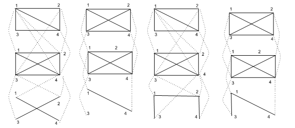 Figure 1
Peer Reviews
No public reviews on file for this paper yet. If you reviewed it on a platform where reviews are public (OpenReview, ICLR, NeurIPS, ICML), you can paste yours below so the community can read it here.
Videos
No videos yet. Explain this paper in a talk, walkthrough, or lecture? Add one.
Layered graphs: a class that admits polynomial time solutions for some hard problems
1,2Bhadrachalam Chitturi
1Department of Computer Science, Amrita Vishwa Vidyapeetham, Amrita University, Amritapuri Campus, Kollam, Kerala 690525, India.
2Department of Computer Science, University of Texas at Dallas, Richardson, Texas 75083, USA.
**Abstract: The independent set on a graph is a subset of such that no two vertices in the subset have an edge between them. The MIS problem on seeks to identify an independent set with maximum cardinality, i.e. maximum independent set or MIS. is a vertex cover if every edge in the graph is incident upon at least one vertex in . is dominating set of if forall either or and . A connected dominating set, CDS, is a dominating set that forms a single component in . The MVC problem on seeks to identify a vertex cover with minimum cardinality, i.e. minimum vertex cover or MVC. Likewise, CVC seeks a connected vertex cover (CVC) with minimum cardinality. The problems MDS and CDS seek to identify a dominating set and a connected dominating set respectively of minimum cardinalities. MVC, CVC, MDS, and CDS on a general graph are known to be NP-complete. On certain classes of graphs they can be computed in polynomial time. Such algorithms are known for bipartite graphs, chordal graphs, cycle graphs, comparability graphs, claw-free graphs, interval graphs and circular arc graphs for some of these problems. In this article we introduce a new class of graphs called a layered graph and show that if the number of vertices in a layer is then MIS, MVC, CVC, MDS and CDC can be computed in polynomial time. The restrictions that are employed on graph classes that admit polynomial time solutions for hard problems, e.g. lack of cycles, bipartiteness, planarity etc. are not applicable for this class.
Key words: Independent set, vertex cover, dominating set, dynamic programming, complexity, polynomial time algorithms. **
1 Introduction
The maximum independent set problem on a graph seeks to identify a subset of with maximum cardinality such that no two vertices in the subset have an edge between them. If is a maximum independent set or MIS for short of then . In this article is undirected, so, an edge is understood to be an undirected edge.
Karp proposed a method for proving problems to be NP-complete [17]. The maximum independent set problem on a general graph is known to be NP-complete [15]. Certain classes of graphs admit a polynomial time solution for this problem. Such algorithms are known for trees and bipartite graphs [1], chordal graphs [2], cycle graphs [3], comparability graphs [6], claw-free graphs [7], interval graphs and circular arc graphs [8]. The maximum weight independent set problem is defined on a graph where the vertices are mapped to corresponding weights. The maximum weight independent set problem seeks to identify an independent set where the sum of the weights of the vertices is maximized. On trees, the maximum independent set problem can be solved in linear time [10]. Thus, for several classes of graphs MIS can be efficiently computed.
Hsiao et al. design an O(n) time algorithm to solve the maximum weight independent set problem on an interval graph with vertices given its interval representation with sorted endpoints list [12]. Several articles improved the complexity of the exponential algorithms that compute an MIS on a general graph [5, 9]. Lozin and Milanic showed that MIS is polynomially solvable in the class of -free planar graphs, generalizing several previously known results where is the graph consisting of three induced paths of lengths 1, 2 and , with a common initial vertex [13].
The minimum vertex cover problem on seeks to identify a vertex cover with minimum cardinality, i.e. minimum vertex cover or MVC. If is MVC of then . In this article is undirected, so, an edge is understood to be an undirected edge. The minimum dominating set, i.e MDS and the minimum connected dominating set i.e. CDS problems seek to identify a dominating set and a connected dominating set respectively of minimum cardinality. The MVC, MDS and CDS probelms on a general graphs are known to be NP-complete [15]. Garey and Johnson showed that MVC is one first NP-complete problem [15]. In connected vertex cover (CVC) problem, given a connected graph G, we are required to find vertex cover set with minimum cardinality such that the induced subgraph G[C] is connected. Garey and Johnson proved that CVC is NP-complete [18]. For trees and bipartite graphs the minimum vertex cover can be identified in polynomial time [20, 21]. Garey and Johnson proved that CVC problem is NP-hard in planar graphs with a maximum degree of 4 [15]. Li et. al. proved that for 4-regular graph CVC problem is NP-hard [19]. It is shown that for series-parallel graphs, which are a set of planar graphs, it shown that minimum vertex cover can be computed in linear time [23].
The minimum dominating set, i.e MDS and the minimum connected dominating set i.e. CDS problems seek to identify a dominating set and a connected dominating set respectively of minimum cardinality. Garey and Johnson showed that MDS on planar graphs with maximum vertex degree 3 and planar graphs that are regular with degree 4 are NP-complete [15]. CDS is NP-complete even for planar graphs that are regular of degree 4 [15]. Bertossi showed that the problem of finding a MDS is NP-complete for split graphs and bipartite graphs [22]. Cockayne et. al. proved that MDS in trees can be computed in linear time [4]. Haiko and Brandstadt showed that MDS and CDS are NP-complete for chordal bipartite graphs [24]. Ruo-Wei et. al. proved that for a given circular arc graph with sorted arcs, CDS is linear in time and space [25]. Fomin et. al. propose an algorithm with time complexity faster than for solving connected dominating set problem [26].
The term layered graph has been used in the literature. The hop-constrained minimum spanning tree problem related to the design of centralized telecommunication networks with QoS constraints is NP-hard [14]. A graph that they call a layered graph is constructed from the given input graph and authors show that hop-constrained minimum spanning tree problem is equivalent to a Steiner tree problem. In software architecture the system is divided into several layers, this has been viewed as a graph with several layers. In this article we define a new class of graphs that we call layered graphs and design an algorithm to identify the corresponding minimum vertex cover.
2 Layered Graph
Consider a set of undirected graphs on the corresponding vertex sets and the edge sets i.e. . Consider a graph that is formed from with special additional edges called inter-layer edges denoted as where and denotes the edges between and . We call such a graph a layered graph denoted as whose layer number is . Note that for any given , where can be and . Every vertex within a given layer gets a label from . Thus, . Note that is the vertex number in layer . However, in layer the vertex number need not exist. Further, if then it follows that vertex is present in layer and vertex is present in layer .
We define the following restrictions on a layered graph. Several of the primary restrictions can be combined. Please see Figure 1.
- •
The size of all graphs is restricted such that then a k-restricted layered graph i.e. is obtained. denotes an with layers. denotes an with vertices.
- •
If for the only permissible edges are where then a linear layered graph i.e. is obtained. denotes an that is k-restricted. denotes an with layers. denotes an with vertices.
- •
If every is required to be a connected component then a single component layered graph i.e. is obtained.
- •
If is required to be a connected component then a connected layered graph i.e. is obtained.
This article primarily studies where every vertex within a given layer gets a label from . The results being general are applicable for , and any combination thereof. Clearly, CDS, CVC are well defined only on ; further, the entire must be a single component. The recursive process of generating a hypercube of dimension i.e. from two copies of consists of creating the inter- edges where and are the corresponding vertices from the first copy of and the second copy of respectively. Thus, the inter-layer edges of are in fact akin to a subset of inter- edges because an inter- edge exists between every pair of corresponding edges. However, in an the successive layers need not have all allowed edges; moreover, and need not be identical.
The complete graph on vertices is known as a clique on vertices and it is denoted by . Consider a graph formed from several copies of say where in addition to the edges that exist in each of an edge is introduced between every pair : and . We denote this particular graph that has layers with . The class of k-restricted layered graphs are in fact subgraphs of . Thus, we call as full . Likewise, a that is defined on cliques where for any for all values of an edge is introduced between vertex of layer and vertex of layer is called as a full . The number of layers in i.e. is bounded by . Likewise, the number of connected components in this graph lie in . Recall that for any given , can be ; that is the adjacent layers need not have any inter-layer edges among them.
A subgraph of induced by vertices consists of all vertices and all the edges defined on them. We design an algorithms that computes the cardinality of a MVC, CDS and CDS of any subgraph of i.e. with polynomial time complexity when . Moreover, we compute the number of MISs, MVCs, CDSs and CDSs in . The worst case time complexity analysis which shows that these problems can be solved in polynomial time for holds for all these problems even though the time complexities are not identical when the parameter is considered.
CDS problem is meaningful only for . However, CVC problem does not require because in the layers with no edges a vertex need not be selected. If every layer has at least one edge then CVC also requires .
3 Algorithm
Consider a layered graph with layers i.e. with layers . We design a generic dynamic programming algorithm for all the problems. The CDS is applicable only when is connected; thus, for these versions we are restricted to . The specific details pertaining to each problem are elucidated. The layers are processed sequentially from the first to the last. Let be a candidate solution for a problem where denotes the set of nodes that are chosen from layer . The candidate sub-solutions or simply for layer and layers are denoted as and respectively where denotes a combined candidate sub-solution for the first layers. Likewise, and denote particular instances where the solution chosen in layer equals i.e. is a -bit variable that we call mask that denotes the chosen vertices. Further, potentially denotes several candidate sub-solutions of vertices from the first layers where is the mask corresponding to the layer . We in general do not even store all these vertex sets but only the cardinality of the best option(s), such cardinality is called an optimum value. This is stored in the variable and the number of solutions that yield the optimum value when the mask for layer is is stored in .
The current layer requires the information only from the previous layer. So, only the variables of the current layer and the previous layer are maintained. The index 0 refers to the variables of the previous layer and index one refers to the same of the current layer. When the information for the index one is completely computed then it is overwritten onto the corresponding variables of index zero; the variables with index one are zeroed out and the next layer is processed (which becomes the current layer). This is a standard technique. Further, the overwriting of variables can be avoided by alternately assigning layers 1 and 0 as the current layer (the other becomes the corresponding previous layer). By employing extra space we can easily keep track of all possible solutions. However, we employ only space (for domination problems we employ space ) in addition to the space required by the graph. If we employ space ( for domination problems, space) where for each mask in each layer we store a best compatible mask from the previous layer then we can additionally generate a solution. However, if we want to generate all solutions then for each mask of a given layer we need to store all compatible masks of the previous layer that yield the optimum value. This further increases the space requirement.
We say that and are compatible if . That is the union of and yields a for the first layers. Note that compatibility is determined by and and the vertices chosen by in the earlier layers is irrelevant. This is a key feature.
3.1 Input
The Input consists of that is specified in terms of and where is the 0-1 adjacency matrix for layer i.e. . is the 0-1 adjacency matrix for . The rows of correspond to the vertices and the columns of are the vertices . It must be noted that for a linear graph can just be a dimensional vector and the corresponding computation is less expensive where an edge between exists. The boolean valued function compatible is called to determine whether candidate sub-solutions (of the current layer and the subgraph induced up to the previous layer) can be combined; here the layer number is implicit. For each mask of a given layer a function determines if is a feasible option for layer . The helper function returns the number of bits that are set in the binary representation of some mask .
All algorithms consist of the following sequence of computational tasks.
- •
Repeat (i) and (ii) for all layers .
- •
(i) Feasible: (if ) then go to step(ii).
- •
(ii) Extension: If and are compatible then store the cardinality of in and the count of in . Corresponding to each if additional variables are present then update them (e.g. DS problems).
- •
(iii) Summarize: Layer execute (i) and (ii). Identify the optimum cardinality among and the corresponding count.
Each problem has specific characteristics. The compatibility criteria and other specifics for each of the problems is elucidated below.
3.2 MIS
Consider the structure of a MIS on say where are the vertices in MIS from layer . Clearly, must be an IS. Let be the subgraph of induced by and let be the subgraph of induced by . Consider the IS of . IF and then and are ISs. Let the set of edges crossing the cut be . It follows that the cardinality of an IS of is when there is no edge crossing . Note that the only edges that can go across the cut are . Thus, the cardinality of MIS of .
- •
: the mask must denote an IS for .
- •
: the union of two ISs must be an IS.
- •
Extension: if .
- •
Summarize: Let ;; ; Return
3.3 MVC and CVC
Consider the VC of where denotes the set of vertices in from layer . Clearly, is a VC for layer . depends only on and .
Consider two adjacent layers and . must cover all edges inter-layer edges between layers and . Specifically, must cover all edges in the corresponding induced subgraph including . Similar constraints hold for CMVC. Additionally the induced subgraph of must be a single connected component.
- •
: the mask must denote a VC for . For CVC must be connected.
- •
: the union of two VCs must be a VC for edges in and .
- •
Extension: if . For CVC masks and must have at least on edge in between.
- •
Summarize: Let ;; ; Return
3.4 MDS and CDS
Let the MDS on say where are the vertices in this MDS from layer . Clearly, need not be a DS of layer because the can be dominated from any of . It follows that must dominate all vertices in layers . Specifically, the inclusion of in must ensure the domination of .
Consider in layer . Say, dominates layer . However, this particular union of vertices leaves certain vertices in layer undominated. The number of such choices are ; each choice is denoted by a k-bit variable that we call mask, here, a mask of exclusion. Further, when one processes layer this information is significant. We show that triples stored for each mask of a given layer suffice to compute MDS (CDC) of . We aim to show that for a chosen mask in layer it suffices to store triples of the form . Here is the mask of the vertices that are not dominated in layer , is the cardinality of the vertices chosen so far and is the number of choices corresponding to for a particular in layer . The particular mask in the previous layer that is the cause for a particular triple in the current layer need not be carried forward. So, for MDS and CDS indicates an array of triples where is the mask of undominated vertices of layer ; are the respective size and count.
Let mask is chosen in layer it potentially be combined with every mask ( masks) of the previous layer. Thus, potentially () triples need be stored. Further, the total number of triples of the form is because can potentially assume any of , is and can in fact be exponential in . Here we make the following critical observations.
- •
Let the chosen mask for layer is . When all the compatible vertex sets of the previous layer are considered then let the resultant triples for the choice of in layer be set .
- •
In for any two triples with the same mask we need only retain the triples with the least size. The other triples cannot lead to an optimum solution.
- •
If two triples have the same mask and the minimum size then they can be combined into one triple where the respective counts are added.
- •
Thus, only triples suffice for a chosen mask for layer . Which implies triples suffice . We store the information of only two layers. Thus, the space complexity is
- •
Thus, for a chosen mask for layer potentially triples of previous layer must be processed. That is, for all masks of layer , triples of previous layer must be processed.
- •
Consider the mask in layer and mask in layer . Recall that there are triples stored corresponding to mask in layer . All the vertices that are covered by the combination of and in layer say and not covered in layer say can be computed in . This needs to be computed only once. Subsequently, for each triples stored corresponding to in layer we need only check if the undominated vertices are a subset of in time. Thus, is the dominating term in the time complexity yielding for all masks of the previous layer. So, for all masks of the current layer the time complexity is . Thus, the time complexity of the algorithm is .
Similar constraints hold for CMDS. Additionally the induced subgraph of must be a single connected component. Thus, is connected. The time and space complexities are identical.
- •
: For CMDS must be connected. For MDS any is valid.
- •
: the union must dominate all vertices of . For CDC masks and must have at least on edge in between.
- •
Extension: Performed as per critical observations listed above. The choice of the final layer must ensure that the final layer is dominated.
- •
Summarize: Let ;; ; Return
3.5 Algorithm Compatible
The function compatible receives two masks denoting chosen vertices from layers and . If the vertices in layer dominate the so far undominated vertices in layer then the function returns true. Otherwise, it returns false.
Algorithm Compatible
1:Input: , , , and . //The function call: . : Mask for layer .
2:Output: 0 (incompatible) or 1 (compatible). //: Mask for layer . denotes matrix for .
3: // returns true if bit is set in else returns false.
4:Case MIS: // Input: two valid MISs of two adjacent layers
5:if then // : for any and :
6: return 1; //if return 0; otherwise return 1; algorithm.
7:else
8: return 0; // a pair of vertices across the layers joined with an edge.
9:end **if
**
10:Case MVC: // Input: two VCs of two adjacent layers
11:if then // : where : or
12: return 1; // then return 1; otherwise return 0; algorithm.
13:else
14: return 0;
15:end **if
**
16:Case CMVC: // Input: two CVCs of two adjacent layers
17:if then // : where : or
18: return 1; // and
19:else // then return 1; otherwise return 0; algorithm.
20: return 0;
21:end **if
**
22:Case MDS: // Input: two masks of two adjacent layers,
23:if then // :
24: return 1; // : if then return 1; otherwise return 0;
25:else // : if then return 1; otherwise return 0;
26: return 0; // or is not dominated. algorithm.
27:end if // is the set of all vertices neighboring any vertex in
28:Case CDS: // Input: two masks of two adjacent layers,
29: //
30:if then // :
31: return 1; // : if then return 1; otherwise return 0;
32:else // : if then return 1; otherwise return 0;
33: return 0; // or is not dominated. algorithm.
34:end if // is the set of all vertices neighboring any vertex in
3.6 Algorithm Generic Optimum
The algorithms for all the problems on is similar. We give a generic dynamic programming based algorithm. Some specific instances are shown in the Appendix. Initialization: ; ; The minimum value of an vertex cover up to layer where the chosen vertices of the layer are given by the binary value of . the number of ways the mask in layer yields the corresponding minimum value. The time complexity for MIS, MVC and CVC is and the space complexity is . The time complexity for MDS and CDS is and the space complexity is .
Algorithm Generic Optimum
Input:
Output: The cardinality and the count for the resp. problem.
for (0,…,) do
if for layer 1 then
// For all valid masks set their count
end if
end for
for () do //For layers 2 through maximum
for do //For all masks of current layer
Compose larger sub-solutions by considering all compatible masks of the
previous layer and any accompanying information.
end for//Masks of previous layer
end for//For all layers
for (i=0,….) do
Identify , the cardinality of the optimum solution.
end for
for () do
Compute , the count of optimum solutions.
end for
4 Correctness and complexity
The correctness is shown for MIS and MVC problems. The time complexities are identical and the analysis is given for MVC. The proofs of correctness for the remaining problems are similar. The time complexity for domination problems was presented earlier.
Theorem 1
Algorithm correctly computes the MIS on .
Proof: Consider the structure of MIS on . Let be the subgraph of induced by and let be the subgraph of induced by . Consider the IS of . Let and be the independent sets of and respectively. Let the set of edges crossing the cut be . It follows that the cardinality of an IS of is when there is no edge crossing . Note that the only edges that can go across the cut are . Thus, the cardinality of MIS of . This, is exactly being computed. The theorem follows. Another proof that can be given for this theorem is based on mathematical induction on subgraphs induced by the first layers. Likewise, gives the number of ways an independent set of maximum cardinality that can be formed when the vertices chosen in the layer are given by . Thus, corresponding to the maximum value of yields the total number of MISs.
Theorem 2
Algorithm correctly computes the MVC on .
Proof: Consider the structure of MVC on . Let be the subgraph of induced by and let be the subgraph of induced by . Consider the VC of . Let and be the vertex covers of and respectively. Let the set of edges crossing the cut be . It follows that the cardinality of an VC of is when every edge crossing is covered by either or . Note that the only edges that can go across the cut are . Thus, the cardinality of MVC of . This, is exactly being computed. The theorem follows. Another proof that can be given for this theorem is based on mathematical induction on subgraphs induced by the first layers. Likewise, gives the number of ways an vertex cover of minimum cardinality that can be formed when the vertices chosen in the layer are given by . Thus, corresponding to the minimum value of yields the total number of MVCs. .
Theorem 3
Algorithm MVC on runs in polynomial time in when . The space required is .
Proof: We presume that , the 0-1 adjacency matrix for the subgraph induced by where the edges are restricted to is given. Likewise, we assume that the 0-1 adjacency matrix for each of are given. Recall that was formed from . For a linear graph, is just a dimensional vector where if bit is set then there is an edge between and .
- •
The initialization step requires time.
- •
Given a mask for layer it can be determined if it is a valid VC in time with . That is, for any two that is set the mask should have either bit or bit set.
- •
Given two masks for layers respectively and it can be directly determined if their union is a VC of a subgraph induced by of in time.
- •
In order to determine the MVC up to layer whose mask is ; must be checked for compatibility with all masks of the previous layer. Thus, time is required. For all masks of the current layer time is required. For all layers, the time required is maximized when each layer has vertices yielding = time.
The time complexity is clearly exponential in ; however, if the time complexity is . The time complexity remains polynomial when . The space required is because for two layers we store mask and count variables each of size .
5 Conclusions
A new large class of graphs called layered graphs have been defined. These graphs can have exponential number of cycles. This class includes a subset of bipartite graphs and a subset of trees on vertices. The restrictions that are employed on graph classes that admit polynomial time solutions for hard problems, e.g. lack of cycles, bipartiteness, planarity etc. are not applicable for this class. The computation of hard problems on these graphs along with the count of the corresponding optimum solutions is shown to be in when layer size is .
6 Acknowledgments
Authors thank Amma for her guidance. This article is based on technical report UTDCS-02-17.
7 Appendix
The generic algorithm was presented earlier. Here, we state two specific algorithms for MIS and MVC respectively.
Algorithm MIS
Input:
Output: The cardinality of MIS and the count of the maximum independent sets.
Initialization: ;
;
// The maximum value of an independent set up to layer where the chosen
//vertices of the layer are given by the binary value of .
// the number of ways the mask in layer yields the corresponding maximum value.
// is a boolean function that returns true if the vertex assignment in the current layer
//corresponding to the binary value of forms an IS. Otherwise it returns false.
// is the bitwise AND operator.
// is the number of bits that are set in the binary representation of .
// For each one -bit variable that remembers the mask of the layer that
// yielded will help in constructing MISs. Union of such masks (1/layer) is an MIS.
// This will require additional space. Current version needs only space.
for (0,…,) do
if for layer 1 then
// No. of valid ISs of layer 1
end if
end for
for () do //For layers 2 through maximum
for do //For all masks of current layer
if then // is valid
for do //Masks of previous layer
if then //Invalid IS
if then // Better IS for the current mask
end if
end if
end for//Masks of previous layer
for do //Masks of previous layer
if () then //Instance of max
// Count corr. to max wrt mask=
end if
end for//Masks of previous layer
end if// is valid
end for//For all masks of current layer
;
end for//For layers 2 through maximum
for (i=0,….) do
if then //Get the max value of
end if
end for
for () do
if then //Corr. to the best value of
//Get the count of MISs
end if
end for
//MIS cardinality and the count of such MISs
Algorithm MVC
Input:
Output: The cardinality and the count for the resp. problem.
for (0,…,) do
if for layer 1 then
// No. of valid VCs of layer 1
end if
end for
for () do //For layers 2 through maximum
for do //For all masks of current layer
if then // is valid
for do //Masks of previous layer
if then //Invalid VC
if then // Better VC for the current mask
end if
end if
end for//Masks of previous layer
for do //Masks of previous layer
if () then //Instance of max
// Count corr. to max wrt mask=
end if
end for//Masks of previous layer
end if// is valid
end for//For all masks of current layer
;
end for//For layers 2 through maximum
for (i=0,….) do
if then //Get the max value of
end if
end for
for () do
if then //Corr. to the best value of
//Get the count of MVCs
end if
end for
//MVC cardinality and the count of such MVCs
The reference list from the paper itself. Each links out to its DOI / PubMed record.
- 1[1] Harary, Frank. Graph theory. 1969.
- 2[2] Gavril, Fanika. Algorithms for minimum coloring, maximum clique, minimum covering by cliques, and maximum vertex cover of a chordal graph. SIAM Journal on Computing 1.2 (1972): 180-187.
- 3[3] Gavril, Fanika. Algorithms for a maximum clique and a maximum independent set of a circle graph. Networks 3.3 (1973): 261-273.
- 4[4] Cockayne, E., Sue Goodman, and Stephen Hedetniemi. A linear algorithm for the domination number of a tree. Information Processing Letters 4.2 (1975): 41-44.
- 5[5] Tarjan, Robert Endre, and Anthony E. Trojanowski. Finding a maximum independent set. SIAM Journal on Computing 6.3 (1977): 537-546.
- 6[6] Golumbic, Martin Charles. The complexity of comparability graph recognition and coloring. Computing 18.3 (1977): 199-208.
- 7[7] Minty, George J. On maximal independent sets of vertices in claw-free graphs. Journal of Combinatorial Theory, Series B 28.3 (1980): 284-304.
- 8[8] Gupta, Udaiprakash I., Der-Tsai Lee, and JY‐T. Leung. Efficient algorithms for interval graphs and circular arc graphs. Networks 12.4 (1982): 459-467.